Gravitational Waves dynamics with Higgs portal and U(1) x SU(2) interactions

Abstract

Finding the origins of the primordial Gravitational Waves (GWs) background by the near-future Cosmic Microwave Background (CMB) polarisation experiments is expected to open a new window Beyond the Standard Model (BSM) of particle physics, allowing to investigate the possible connections between the Electroweak (EW) symmetry breaking scale and the energy scale of inflation. We investigate the GWs dynamics in a set-up where the inflation sector is represented by a mixture of the SM Higgs boson and an U(1) scalar singlet field non-minimally coupled to gravity and a spectator sector reprezented by an U(1) axion and a SU(2) non-Abelian gauge field, assuming that there is no coupling, up to gravitational interactions, between inflation and spectator sectors.

We show that a mixture of Higgs boson with a heavy scalar singlet with large vacuum expectation value (vev) is a viable model of inflation that satisfy the existing observational data and the perturbativity constraints, avoiding in the same time the EW vacuum metastability as long as the Higgs portal interactions lead to positive tree-level threshold corrections for SM Higgs quartic coupling.
We evaluate the impact of the Higgs quartic coupling threshold corrections on the GW sourced tensor modes while accounting for the consistency and backreaction constraints and show that the Higgs portal interactions enhance the GW signal sourced by the gauge field fluctuations in the CMB B-mode ploarization power spectra.

We address the detectability of the GW sourced by the gauge field fluctuations in presence of Higgs portal interactions for the experimental configuration of the future CMB polarization LiteBird space mission. We find that the sourced GW tensor-to-scalar ratio in presence of Higgs portal interactions is enhanced to a level that overcomes the vacuum tensor-to-scalar ratio by a factor ${\mathcal{O}}(10)$, much above the detection threshold of the LiteBird experiment, in agreement with the existing observational constraints on the curvature fluctuations and the allowed parameter space of Higgs portal interactions.

A large enhancement of the sourced GW can be also detected by experiments such as pulsar timing arrays and laser/atomic interferometers. Moreover, a significant Higgs-singlet mixing can be probed at LHC by the measurement of the production cross sections for Higgs-like states, while a significant tree level threshold correction of the Higgs quartic coupling can be measured at colliders by ATLAS and CMS experiments.

1 Introduction

Detection of the primordial Gravitational Wave (GWs) background would provide strong evidence for the existence of the cosmic inflation [1, 2, 3]. The properties of scalar density fluctuations measured by the Cosmic Microwave Background (CMB) experiments are in agreement with the main predictions of the simplest models of inflation [4, 5, 6] while the CMB polarization data place constraints on the primordial tensor modes [7].
The amplitude of the GWs background is parameterized by the tensor-to-scalar ratio $r$, the ratio of the amplitudes of tensor and scalar power spectra of density fluctuations. Currently, the tightest upper bound on tensor-to-scalar ratio i$r<0.036$ at 95% confidence is placed from the combined analysis of Planck and BICEP2/Keck array [9].
The detection of the GWs background is likely to come from the future CMB B-mode polarization experiments, such as the LiteBIRD satellite experiment [10, 11] and the ground-based CMB-S4 experiment [12] expected to measure the tensor-to-scalar ratio with a sensitivity $\delta r<10^{-3}$.

However, the detection of $r$ is not enough to discriminate among the possible origins of the GWs background.
In the standard scenario where inflation is driven by a slow rolling scalar field minimally coupled to gravity, the GWs background is produced by the quantum vacuum fluctuations of the metric [1, 13, 14] and the tensor-to-scalar ratio can be directly related to the Hubble expansion rate $H$ during inflation [15]. The current upper bound on tensor-to-scalar ratio gives $H<4.37\times 10^{13}$ GeV. In this scenario the GW power spectrum is nearly scale-invariant, nearly Gaussian and parity-conserving (non-chiral).

This does not hold if the tensor modes are produced by the mater gauge fields during inflation.
One of the most studied mechanisms leading to successfully production of sourced GW by the matter fields involves SU(2) non-Abelian massless gauge fields. In this scenario the amplification of fluctuations in the gauge field sector, with subsequent enhancement of the tensor modes during inflation, is realized breaking the conformal invariance of the gauge field by coupling with an U(1) pseudo-scalar axion field via the Chern-Simons interaction term [16, 17]. This configuration leads to an isotropic and spatially homogeneous cosmological solution where isotropy is protected by the non-Abelian gauge field invariance [17].
The tensor modes generated by this mechanism can leave distinctive signatures in the primordial GWs background compared to the vacuum fluctuations of the metric. The sourced GWs are scale-dependent [56], strongly non-Gaussian [18, 19, 20, 21, 22] and parity-beaking [23, 24, 52]. However, this model results in too red spectrum of the scalar perturbations (too small scalar spectral index) if the constraint on axion decay constant $f<M_{pl}$ is respected ($M_{pl}$ is the Planck mass) and is excluded by the observations [25, 26, 74].

Accommodation of the observational bounds for the scalar and tensor modes while the gauge fields play an important role in production of cosmological perturbations is challenging. During inflation a large amount of spin-2 particles produced to source the GWs background at observational level causes backreactions on dynamics of the axion-gauge fields [54, 61, 62, 70] that can result in predictions for cosmological observables ruled out by the experimental measurements. The solution was to consider the axion-gauge field sector as spectator, decoupled up to gravitational interactions from the inflation sector [56], set-up used by most of the sourced GWs studies in context of the standard inflation [54, 62, 70, 72].

Finding the GW origin by using the CMB polarisation measurements is expected to open a new window beyond the Standard Model (BSM) of particle physics, allowing to investigate the possible connections between the energy scale of inflation and the subsequent energy scales in the evolution of the Universe.

The discovery by the Large Hadron Collider (LHC) of the Higgs boson [27, 28] increased the interest in so called Higgs portal interactions that connect the hidden (dark) and visible sectors of the Standard Model (SM). Scenarios beyond-the-SM (BSM), that introduce a dark sector in addition to the visible SM sector are required to explain a number of observed phenomena in particle physics, astrophysics and cosmology such as non-zero neutrino masses and oscillations, nature of Dark Matter (DM), baryon asymmetry of the Universe, cosmological inflation [29].
In the original Higgs inflation model [30, 31] the SM Higgs boson can play the role of inflaton if it has a large non-minimal coupling to gravity $\xi\sim{\cal O}(10^{5})$. The model predictions are consistent with cosmological data [7], suggesting possible connections between electroweak (EW) scale and the inflation scale. However, for such large values of $\xi$ the unitary bound scale $\Lambda_{U}\sim M_{pl}/\xi$ could be close or much below the energy scale of inflation. Such large couplings can be generated at Renormalisation Group (RG) loop levels, but in this case the price to pay is the vacuum metastability, as the SM Higgs quartic coupling becomes negative due to the radiative corrections [32, 33].

Higgs portal interactions allow to build viable inflation models where the inflaton role is played by a mixture of Higgs boson with a singlet scalar field with non-zero vacuum expectation value (vev) non-minimally coupled to gravity [34, 38, 48]. Such models are in agreement with the CMB observations [7] and satisfy the perturbativity and the tree-level unitarity constraints as long as the effective mixing coupling $\lambda_{hs}$ is sufficiently small. The Higgs-scalar singlet mixture leads to positive tree-level threshold correction to the Higgs quartic coupling, preventing in this way the EW vacuum metastability [34, 35, 38].

Higgs-scalar singlet models are also attractive from the standpoint of the GW production as they predict strong first-order cosmological phase transitions (PTs) at the EW scale, leading to detectable GW signal. The PT can be generated when the scalar field experiences a change in its vev in a certain temperature range, undertaking a transition into a new phase by quantum or thermal processes. This process proceed by the nucleation of bubbles in plasma through: (b) collisions of expanding bubble walls, (s) sound waves produced by the bulk motion in plasma after the bubbles have collided but before expansion has dissipated the kinetic energy and (t) magnetohydrodynamic turbulence in plasma after the bubbles have collided (for details see Ref. [39] and references therein). As these processes coexist, the present GW energy density spectrum can be approximated as a linear combination of the contributions from the above mechanisms: $\Omega_{GW}$=$\Omega_{b}$+$\Omega_{s}$+$\Omega_{t}$.
The peak-integrated sensitivity curves (PISCs) for $\Omega_{b}$, $\Omega_{s}$ and $\Omega_{t}$ obtained in the Higgs-scalar singlet model, corresponding to different future GW searches, are given in Refs. [41, 42].
The analysis of the effects of the Higgs-scalar singlet couplings on the EW phase transition, including the dimension-six non-renormalizable operators to couple the singlet scalar field with the SM Higgs doublet [40], shows that the EW phase transition can occur in two-steps, a singlet phase transition at high temperature and a subsequent strong first-order phase transition in SM sector. This scenario can explain the baryon asymmetry in the Universe and is compatible with scalar singlet as Dark Matter candidate with a mass nearly half of the Higgs mass.
The consequences of the EW symmetry breaking on GW energy spectrum in presence of axion-Higgs non-perturbative couplings were recently analyzed in context of $R^{2}$ inflation and Einstein-Gauss-Bonnet inflation models [43, 44].

A significant Higgs-singlet mixing can be probed at LHC by measurement of the production cross sections for Higgs-like states [45, 37]. Furthermore, the Higgs-singlet mixing can lead to a significant tree level modification of the Higgs quartic coupling, which can be measured at colliders [27, 28].

In this paper we investigate a scenario where the axion and non-Abelian gauge fields are confined to the spectator sector while the inflation sector is represented by a mixture of Higgs and a scalar singlet field non-minimally coupled to gravity. We show that the Higgs portal interactions lead to positive tree-level threshold corrections to SM Higgs quartic coupling leading to the change of the Hubble expansion rate during inlation. This impacts on the evolution of the axion-gauge field spectator sector modifying the time-dependent mass parameter of the gauge field fluctuation.
We assume that there is no coupling, up to gravitational interactions, between inflation and spectator sectors and the background energy density is dominated by inflation. The relevant Jordan frame action of the model, where hat is representing the quantities in the Jordan frame, is given below:

$${\cal S}_{J} = \int{\rm d}^{4}x\sqrt{-{\hat{g}}}\,[\frac{1}{2}(M^{2}_{pl}+\xi_{h}h^{2}+\xi_{s}s^{2}){\cal{\hat{R}}}$$ (1)

$$- \underbrace{\frac{1}{2}(\partial_{\mu}h)^{2}-\frac{1}{2}(\partial_{\mu}s)^{2}+V(h,s)}_{{\cal L}_{inf}}-\underbrace{\frac{1}{2}(\partial\hat{\chi})^{2}-V_{a}(\hat{\chi})-\frac{1}{4}\hat{F}^{a}_{\mu\nu}\hat{F}^{a\mu\nu}+{\hat{\cal L}}_{int}}_{{\cal L}_{spec}}]\,.$$

Here $\hat{g}$ is the determinant of the metric tensor, $M_{pl}$ is the Planck mass, ${\cal{\hat{R}}}$ is the Ricci curvature, $\xi_{h}$ and $\xi_{s}$ are the couplings of Higgs and scalar fields with the curvature, $V(h,s)$ is the inflaton potential, $V_{a}(\hat{\chi})$ is the axion potential and $\hat{F}^{a}_{\mu\nu}$ is the gauge strength field tensor. The axion field is expected to interact with the gauge fields through the Chern-Simons interaction term $\hat{\cal L}_{int}$. Transition of the action (1) from the Jordan to the Einstein frame is accomplished by rescaling the metric:

$$g_{\mu\nu}=\Omega{\hat{g}}_{\mu\nu}\,,\hskip 17.07182pt\Omega(h,s)=(M^{2}_{pl}+\xi_{h}h^{2}+\xi_{s}s^{2})\,.$$ (2)

We study the dynamics of the axion-gauge field spectator in presence of Higgs portal interactions in a comprehensive parameter space for two slow-roll solutions for the mass parameter of gauge field fluctuations [62] while accounting for consistency and backreaction constraints.
The most interesting result obtained is the enhanced production of the sourced GW by the non-Abelian gauge field in presence of Higgs portal interactions to a level that overcomes the quantum vacuum fluctuations by a factor ${\mathcal{O}}$(10) for both solutions, much above the detection threshold of the near-future B-modes polarization experiments, in agreement with the CMB observations on curvature fluctuations and with the allowed parameter space of Higgs portal interactions.

The paper is organized as follows. In section 2 we review the Higgs-singlet inflation model and place constraints on Higgs portal parameter space requiring the agreement with the observations on curvature fluctuations. In section 3 we present the Higgs-singlet inflation model with transiently rolling U(1) x SU(2) spectator fields and analyse the consistency and backreaction constraints. Section 4 is dedicated to provide constraints on the parameter space of the spectator axion-gauge field model in presence of Higgs portal interactions. We present our conclusions in section 5.

Throughout the paper we consider an homogeneous and isotropic background described by the Friedmann-Robertson-Walker (FRW) metric and work in natural units ($\hbar$=$c$=$M_{pl}$=1) unless specified otherwise.

2 Higgs-scalar singlet inflationary dynamics

Extension of the Higgs sector with a real scalar field in presence of the large couplings to scalar curvature can lead to inflation based on scale invariance of the Einstein frame scalar potential at large field values. As in the case of Higgs inflation [30, 31] the potential becomes exponentially flat at large field values that is favoured by the inflationary observables [7]. Below we summaise the basic ideas of the Higgs-scalar singlet inflation, following Refs. [34, 38].

We assume a ${\mathbb{Z}}_{2}$-symmetric inflation potential of the form:

$$V(h,s)=\frac{1}{4}\lambda_{h}h^{4}+\frac{1}{4}\lambda_{hs}h^{2}s^{2}+\frac{1}{4}\lambda_{s}s^{4}+\frac{1}{2}m^{2}_{h}h^{2}+\frac{1}{2}m^{2}_{s}s^{2}\,,$$ (3)

where $m_{h}$ and $m_{s}$ are $h$ and $s$ fields masses, $\lambda_{h}$ and $\lambda_{s}$ are their quartic couplings and $\lambda_{hs}$ is the mixing quartic coupling. Here after we will consider that both fields develop non-zero vacuum expectation values (${\it vev}$) denoted by $<h>={\it v}$, $<s>={\it w}$ and $w\gg{\it v}$. We will also consider large field values and $\xi_{h}\gg\xi_{s}$ such that:

$$\xi_{h}h^{2}+\xi_{s}s^{2}\gg 1\,,\hskip 28.45274pt\xi_{h}+\xi_{s}\gg 1\,.$$ (4)

After the conformal transformation given in Eq. (2), the kinetic term and the inflation potential in the Einstein frame read as [34]:

$${\cal L}_{kin} = \frac{1}{2}(\partial_{\mu}\phi)^{2}+\frac{1}{2}\frac{\xi^{2}_{h}\tau^{2}+\xi_{s}^{2}}{(\xi_{h}\tau^{2}+\xi_{s})^{3}}(\partial_{\mu}\tau)^{2}\,,$$ (5)

$$U(\tau) = \frac{\lambda_{h}\tau^{4}+\lambda_{hs}\tau^{2}+\lambda_{s}}{4(\xi_{h}\tau^{2}+\xi_{s})^{2}}\,,$$ (6)

where the new variables $\phi$ and $\tau$ are defined as:

$$\phi=\sqrt{\frac{3}{2}}\log{(\xi_{h}h^{2}+\xi_{s}s^{2})}\,,\hskip 28.45274pt\tau=\frac{h}{s}\,.$$ (7)

The minima of the potential given in Eq. (6) are classified in Refs. [34, 38] according to the particle content during inflation. For Higgs-singlet inflation to occur the following conditions are required:

$$2\lambda_{h}\xi_{s}-\lambda_{hs}\xi_{h}>0\,,\,\,\,2\lambda_{s}\xi_{h}-\lambda_{hs}\xi_{s}>0\,,\,\,\,\tau_{min}=\sqrt{\frac{2\lambda_{s}\xi_{h}-\lambda_{hs}\xi_{s}}{2\lambda_{h}\xi_{s}-\lambda_{hs}\xi_{h}}}\,,$$ (8)

As $\tau\sim M_{pl}/\sqrt{\xi_{h}}$ it can be integrated out in Eq. (5), leaving $\phi$ the only dynamical variable during inflation. Details of this computation can be found in Refs. [34, 38, 45, 46].

The potential for $\phi$ can be written as:

$$U(\phi)=\frac{\lambda_{eff}}{4\xi^{2}_{h}}\left(1+\exp{\left(-\frac{2\phi}{\sqrt{6}}\right)}\right)^{-2}\,,$$ (9)

where $\lambda_{eff}$ is given by:

$$\lambda_{eff}=\frac{1}{4}\frac{4\lambda_{s}\lambda_{h}-\lambda^{2}_{hs}}{\lambda_{s}+\lambda_{h}x^{2}-\lambda_{hs}x}\,,\hskip 14.22636ptx=\frac{\xi_{s}}{\xi_{h}}\,.$$ (10)

The potential from Eq. (9) leads to the following slow-roll parameters:

$$\epsilon_{\phi} = \frac{1}{2}\left(\frac{U_{\phi}(\phi)}{U(\phi)}\right)^{2}\simeq\frac{4}{3}\exp{\left(-\frac{4\phi}{\sqrt{6}}\right)}\,,$$ (11)

$$\eta_{\phi} = \frac{U_{\phi,\phi}(\phi)}{U(\phi)}\simeq-\frac{4}{3}\exp{\left(-\frac{2\phi}{\sqrt{6}}\right)}\,,$$ (12)

where we denote $U_{\phi}(\phi)\equiv\partial U(\phi)/\partial\phi$ and $U_{\phi,\phi}(\phi)\equiv\partial U_{\phi}(\phi)/\partial\phi$.
During inflation $e^{\phi}\gg 1$ and $\epsilon_{\phi}\,,\eta_{\phi}\ll 1$. Inflation ends when $\epsilon_{\phi}\simeq 1$ corresponding to:

$$\phi_{end}\simeq\sqrt{\frac{3}{4}}\ln{\frac{4}{3}}$$ (13)

The number of e-folds before the end of inflation can be obtained as:

$$N=-\int^{\phi_{end}}_{\phi_{in}}\frac{U(\phi)}{U_{\phi}(\phi)}\,\,{\rm d}\phi\simeq\frac{3}{4}\exp{(2\phi_{in}/\sqrt{6})}\,,$$ (14)

leading to the value of the field at beginning of inflation:

$$\phi_{in}\simeq\frac{\sqrt{6}}{2}\ln{\frac{4N}{3}}\,.$$ (15)

For $N=59$ e-folds, as required by the Planck normalization [8], $\phi_{in}=5.34M_{pl}$, while the value of the inflaton field $\phi_{*}$ corresponding to the Hubble crossing of the largest observable CMB scale at $N\simeq 55$ e-folds before the end of inflation [7] is $\phi_{*}=5.26M_{pl}$.

The power spectra of curvature and tensor perturbations generated during inflation by the quantum vacuum fluctuations are:

$${\cal P}^{v}_{{\cal\zeta}}(k) = A_{s}\left(\frac{k}{k_{0}}\right)^{n_{s}-1}\,,\hskip 14.22636ptA_{s}=\frac{H^{2}}{24\pi^{2}\epsilon_{\phi}}\,,$$ (16)

$${\cal P}^{v}_{t}(k) = A_{t}\left(\frac{k}{k_{0}}\right)^{n_{t}}\,,\hskip 28.45274ptA_{t}=\frac{2H^{2}}{\pi^{2}}\,,$$ (17)

where $A_{s}$ and $A_{t}$ are the scalar and tensor power spectra amplitudes, $n_{s}$ and $n_{t}$ the corresponding spectral indexes and $k_{0}$ is the pivot scale. The vacuum tensor-to-scalar ratio at $k_{0}$ is defined as $r^{(v)}_{k_{0}}={\cal P}^{(v)}_{t}/P^{(v)}_{\cal R}$.

To the first order in slow-roll approximation, $n_{s}$, $n_{t}$ and $r^{vac}$ are:

$$n_{s}\simeq 1-6\epsilon_{\phi}+2\eta_{\phi}\,,\hskip 14.22636ptn_{t}=-2\epsilon_{\phi}\,,\hskip 14.22636ptr^{vac}=16\epsilon_{\phi}\,,$$ (18)

leading to $n_{s}=0.961$ and $r^{(v)}=3.44\times 10^{-3}$ for $\phi_{*}=5.26M_{pl}$. The best fit of Planck measurements in the standard $\Lambda CDM$ cosmology indicates ${\cal P}^{obs}_{\zeta}=(2.1\pm 0.03)\times 10^{9}$ and $n_{s}=0.9649\pm 0.0042$ (65% CL) at $k_{0}=0.05$Mpc^-1 [7, 8] while the joint analysis of BICEP2/KECK and Planck data constrained the vacuum tensor-to-scalar ratio $r^{(v)}_{0.05}<0.036$ ( 95% CL) [9].

2.1 Higgs portal assisted Higgs-singlet inflation

Higgs portal interaction term $V(h,s)\subset\lambda_{h,\phi}h^{2}s^{2}$ from Eq. (3) has distinct contributions to both EW scale and to the high energy scales, ensuring the the stability of the inflation potential.
In the limit $\lambda_{s}{\it w^{2}}\gg{\lambda_{h}\it v^{2}}$, the extremization of the scalar potential $V(h,s)$ leads to the squared Higgs mass eigenvalue [34, 35]:

$$m^{2}_{h}\simeq 2{\it v^{2}}\left[\lambda_{h}-\frac{\lambda^{2}_{hs}}{4\lambda_{s}}\right]\,,$$ (19)

$m_{s}^{2}=2\lambda_{s}{\it w}^{2}+2(\lambda^{2}_{hs}/\lambda_{s}){\it v}^{2}$ and mixing angle $\tan 2\theta=\lambda_{hs}{\it v}{\it w}/(\lambda_{h}{\it v}^{2}-\lambda_{s}{\it w}^{2})$.

The Higgs ${\it vev}$ is fixed at ${\it v}\equiv(\sqrt{2}G_{F})^{1/2}$= 246.22 GeV by the Fermi constant $G_{F}$ while the measured SM Higgs mass is $m^{SM}_{h}=125.10$ GeV [37] leading to $\lambda^{SM}_{h}\simeq 0.128$. As a result, Eq. (19) shows that the same value of $m^{SM}_{h}$ can be obtained for various values of $\lambda_{h}$ as long as $\lambda_{h}-\lambda^{2}_{hs}/\ 4\lambda_{s}\simeq\lambda^{SM}_{h}$.
Consequently, at the EW scale the quartic couplings $\lambda_{i}$ are all positive while the perturbativity constraint ($\lambda^{2}_{i}/4\pi<1$) imposes $\lambda_{i}<1$. Therefore, in the Higgs-singlet inflation the Higgs quartic coupling is given by:

$$\lambda_{h}\bigg{|}_{Higgs+singlet}=\lambda^{SM}_{h}+\frac{\lambda^{2}_{hs}}{4\lambda_{s}}\,.$$ (20)

This threshold effect occurs at tree level, avoiding the instability of the EW vacuum and is dominant over quantum loop contributions. Moreover, the size of the shift $\lambda_{hs}^{2}/4\lambda_{s}$ does not depend on the singlet mass, allowing to prevent the potential instability at large field values [35].

On the other hand, the couplings that appear in the inflation potential, including the non-minimal couplings $\xi_{h}$ and $\xi_{s}$, are associated to different energy scales encoded in the renormalisation group (RG) equations [47, 48, 49]. Connecting small and large scales in the large field limit $\xi_{h}\phi^{2}+\xi_{s}s^{2}\gg 1$ can be challenging as the scalar propagators are modified by the curvature term and RG equations receive corrections from higher dimensional operators that can not be calculated reliably [34, 38].

In what follows we do not impose quantum corrections to the Higgs-singlet model. Instead we evaluate $\lambda_{h}$ at EW scale considering the threshold effect given by Eq. (20).
We adopt the Planck normalisation ${\cal P}^{obs}_{\zeta}$ at $k_{0}=0.05$ Mpc^-1 to fix the ratio $U(\phi)/\epsilon_{\phi}=24\pi^{2}{\cal P}^{obs}_{\zeta}$ [30] and evaluate the parameter space allowed by Higgs-singlet model taking as target model the standard $\Lambda CDM$ model with the best fit parameters obtained by Planck [8].
Our numerical analysis is done as follows. We choose $\lambda_{s}$ and $\lambda_{hs}$ as free parameters in the range $0<\lambda_{i}<1$ and take $\xi_{h}$ as free parameter while $\xi_{s}$ is constraint by $\lambda_{hs}\xi_{h}/2\lambda_{h}<\xi_{s}<2\lambda_{s}\xi_{h}/\lambda_{hs}$ as required by Eq. (8).
We modify the original CAMB code [50] to numerically compute the slow-roll parameters and inflationary observables $A_{s},n_{s},r_{v}$ for Higgs-singlet model at $k_{0}=0.05Mpc^{-1}$ and use the Monte-Carlo Markov Chains technique to sample from the space of Higgs-singlet inflation model parameters and generate estimates of their posterior distributions. The tensor spectral index $n^{v}_{t}$ is obtained from the consistency relation $n^{v}_{t}=-r^{v}/8$. We assume a flat universe and uniform priors for all free parameters adopted in the analysis.
Left panel from Figure 1 presents the posterior likelihood probability distributions for the Higgs-singlet model parameters. Requirement that Planck normalisation should be satisfied results in tight constraints for all parameters.
The confidence intervals (at 99% CL) of parameters that we will use in this analysis are given below:

$$\lambda_{hs} : \hskip 14.22636pt4.7\times 10^{-2}\,\,\,\div\,\,\,5.2\times 10^{-2}$$ (21)

$$\lambda_{s} : \hskip 14.22636pt1.5\times 10^{-2}\,\,\,\div\,\,\,1.9\times 10^{-2}$$

$$\xi_{h} : \hskip 14.22636pt1.469\times 10^{4}\,\,\,\div\,\,\,1.473\times 10^{4}$$

$$\xi_{s} : \hskip 14.22636pt2.39\times 10^{3}\,\,\,\div\,\,\,2.83\times 10^{3}\$$

$$H_{inf} : \hskip 14.22636pt2.94\times 10^{-6}M_{pl}\,\,\div\,\,7.02\times 10^{-6}M_{pl}$$

Here $H_{inf}$ is a derived parameter evaluated at $\phi_{*}=5.26\,M_{pl}$ corresponding to the Hubble crossing of the largest observable CMB scale at $N\simeq 55$ e-folds before the end of inflation [7]. The right panel from Figure 1 shows the evolution of the Hubble expansion rate during inflation $H_{inf}$ with $\lambda_{hs}$ for increasing values of $\lambda_{s}$. The figure shows that $H_{inf}$ increases when the tree-level threshold corrections to SM Higgs quartic coupling are decreased.

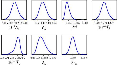
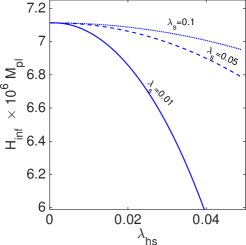
Figure 1: Left: The marginalised likelihood probability distributions obtained for Higgs-singlet inflation model parameters. Right: Evolution of the Hubble expansion rate during inflation $H_{inf}$ with $\lambda_{hs}$ for different values of $\lambda_{s}$. Here $H_{inf}$ is evaluated at $\phi_{*}=5.26\,M_{pl}$ corresponding to the Hubble crossing of the largest observable CMB scale at $N\simeq 55$ e-folds before the end of inflation [7].

We show that a mixture of Higgs boson with a heavy scalar singlet with large vev is a viable model of inflation that satisfy the Planck data constraints avoiding at the same time the instability of the EW vacuum as log as the Higgs portal interactions lead to a positive tree-level threshold corrections for SM Higgs quartic coupling. Moreover, these corrections lead to changes of the Hubble expansion during inlation that impact on the evolution of the axion-gauge field spectator sector.

We evaluate the scalar-singlet mass $m_{s}$ and mixing angle $|\sin(\theta)|$ for $\lambda_{s}$ and $\lambda_{hs}$ in the confidence intervals given in Eq. (21). The best fit vales $(\lambda_{s},\lambda_{hs})=(0.1,0.05)$ lead to $m_{s}=289.42$ GeV and $|\sin(\theta)|=0.122$.
One should note that for $m_{s}\simeq 290$ GeV the maximal allowed mixing angle is $|\sin(\theta)|_{max}=0.31$ and the maximal and minimal allowed branching ratios are $BR^{H\rightarrow hh}_{max}=0.4$ and $BR^{H\rightarrow hh}_{min}=0.18$ at 95% CL [37] while the upper bound of the invisible Higgs boson branching ratio is $BR^{H\rightarrow hh}_{inv}<0.11$ at 95% CL [40]. Figure 2 presents $m_{s}$ - $|\sin(\theta)|$ dependences obtained in Higgs-scalar singlet model for $\lambda_{s}$=0.1 and $\lambda_{s}$=0.2 when $\lambda_{hs}$ is allowed to vary, compared with the maximal allowed values for $|\sin(\theta)|$ in the scalar-singlet high mass region $m_{s}\in[125-600]$ GeV from direct LHC Higgs searchers [36]. The figure clearly shows that the Higgs-singlet mixing can lead to a significant tree-level modification of the Higgs quartic coupling which can be measured at colliders [27, 28].

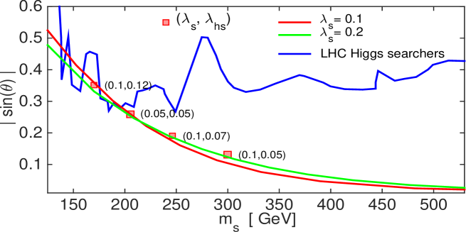
Figure 2: Maximal allowed values for $|\sin(\theta)|$ in the scalar-singlet high mass region $m_{s}\leavevmode\nobreak\ \in\leavevmode\nobreak\ [125-600]$ GeV from the direct LHC Higgs searchers [36] (blue) compared with $m_{s}$ and $|\sin(\theta)|$ values obtained in Higgs-scalar singlet model for $\lambda_{s}$=0.1 (red) and $\lambda_{s}$=0.2 (green) when $\lambda_{hs}$ is allowed to vary in the confidence interval given in Eq. (21). Some particular values $(\lambda_{s},\lambda_{hs})$ are also indicated. The figure shows that the Higgs-singlet mixing can lead to a significant tree-level modification of the Higgs quartic coupling which can be measured at colliders [27, 28].

3 Higgs-singlet inflation with transiently rolling U(1) x SU(2) spectator fields

Throughout we will assume that the total energy density is dominated by the energy density of the inflaton field and treat the Hubble expansion rate $H$ as constant during inflation. More specifically we will take the value of $H$ at $\phi_{*}=5.26M_{pl}$ corresponding to the Hubble crossing of the largest observable CMB scale at $N\simeq 55$ e-folds before the end of inflation.

We briefly review the main features of Higgs-singlet inflation in presence of the axion-gauge fields spectator [51, 52, 53]. The Einstein frame Lagrangian of the model is given by:

$${\cal L}=\frac{1}{2}{\cal R}-\frac{1}{2}(\partial\phi)^{2}-U(\phi)-\frac{1}{2}(\partial\chi)^{2}-V(\chi)-\frac{1}{4}F_{\mu\nu}\tilde{F}^{\mu\nu}+{\cal L}_{int}\,,$$ (22)

where $\phi$ is the inflaton field and $U(\phi)$ is its potential as given in Eq. (7) and Eq. (9), $\chi$ is the axion field endowed with shift symmetry guaranteed by the U(1) gauge invariance, $V(\chi)$ is the axion potential, $F_{\mu\nu}=\partial_{\mu}A_{\nu}-\partial_{\nu}A_{\mu}-g\epsilon^{abc}A^{b}_{\mu}A^{c}_{\nu}$ is the strength of a non-abelian SU(2) gauge field and ${\tilde{F}}^{\mu\nu}\equiv\eta^{\mu\nu\rho\upsilon}F_{\rho\upsilon}/(2\sqrt{g})$ is its dual, where $\eta^{\mu\nu\rho\sigma}$ is an antisymmetric tensor satisfying $\eta^{0123}=g^{-1}$ and $g$ is the gauge coupling.
The axion field is expected to interact with the gauge field through a Chern-Simons term of the form:

$$L_{int}=-\lambda\frac{\chi}{f}F_{\mu\nu}\tilde{F}^{\nu\mu}\,,$$ (23)

where $\lambda$ is a dimensionless coupling constant and $f$ is the axion decay constant of mass dimension.
To minimize the influence of spectator sector on the curvature perturbations generated during inflation and to render the sourced GW produced by the gauge-fields viable we will consider a model that can lead to localized gauge field production where the spectator axion transiently rolls on potential of the form [55, 56, 57]:

$$V(\chi)=\mu^{4}\left[1+\cos{\left(\frac{\chi}{f}\right)}\right]\,,$$ (24)

where $\mu$ is its modulation amplitude with mass dimension. The axion field rolls between $\chi_{min}$=0 and $\chi_{max}=\pi f$ with a velocity that obtains the maximum value at $t_{*}$ when $\chi_{*}=0.5\pi f$ and the slope of the axion potential $V_{\chi}(\chi_{*})$ is maximal. Here $V_{\chi}\equiv\partial_{\chi}V/\partial\chi$.

We assume an initial gauge field configuration described by [51, 58, 59]:

$$A^{a}_{0}=0\,,\hskip 17.07182ptA^{a}_{i}=\delta^{a}_{i}a(t)Q(t)\,,$$ (25)

where $a(t)$ is the scale factor and $Q(t)$ is the SU(2) gauge field. This configuration leads to an isotropic and spatially homogeneous cosmological solution where isotropy is protected by the non-Abelian gauge field invariance [17].

The time-dependent components of the axion-gauge field model $X=(\chi,Q,f)$ translate from Jordan to Einstein frame under the conformal transformation given by Eq.(2) as $\partial X/\partial{\hat{X}}=\Omega^{-1/2}$ where $\hat{X}$ denote the Jordan frame counterpart [60].
In the large-field approximation given by Eq (4) this leads to $\Omega^{-1/2}\simeq\exp{\left(-2\phi_{*}/\sqrt{6}\right)}\simeq 1.36\times 10^{-2}$, leaving the evolution equations of the axion-gauge field spectator unchanged.

The evolution equations of the Hubble parameter reads as:

$$3H^{2} = \frac{1}{2}{\dot{\chi}}^{2}+V(\chi)+\frac{1}{2}{\dot{\phi}}^{2}+U(\phi)+\frac{3}{2}\left[({\dot{Q}}+HQ)^{2}+g^{2}Q^{4}\right]\,,$$ (26)

and the equations of motion for inflaton, axion, and gauge fields without beackreaction are given by [54, 61, 62]:

$${\ddot{\phi}}+3H{\dot{\phi}}+U_{\phi}(\phi) = 0\,,$$ (27)

$$\ddot{\chi}+3H\dot{\chi}+V_{\chi}(\chi) = -\frac{3g\lambda}{f}Q^{2}(\dot{Q}+HQ)\,,$$ (28)

$$\ddot{Q}+3H\dot{Q}+(\dot{H}+2H^{2})Q+2g^{2}Q^{3} = g\frac{\lambda}{f}\dot{\chi}Q^{2}\,.$$ (29)

The Hubble slow-roll parameter $\epsilon_{H}$ contains contributions from inflaton, axion and gauge fields:

$$\epsilon_{H}=\epsilon_{\phi}+\epsilon_{\chi}+\epsilon_{Q_{E}}+\epsilon_{Q_{B}}\,,$$ (30)

where the corresponding slow-roll parameters:

$$\epsilon_{\phi}=\frac{{\dot{\phi}}^{2}}{2H^{2}}\,,\hskip 8.5359pt\epsilon_{\chi}=\frac{{\dot{\chi}}^{2}}{2H^{2}}\,,\hskip 8.5359pt\epsilon_{Q_{E}}=\frac{({\dot{Q}}+HQ)^{2}}{H^{2}}\,,\hskip 8.5359pt\epsilon_{Q_{B}}=\frac{g^{2}Q^{4}}{H^{2}}\,,$$ (31)

are assumed to be smaller than unity during inflation. These parameters modify $\epsilon_{H}$ in Eq. (30), that in turn affects the spectral index of scalar perturbations [54, 70, 71]:

$$n_{s}-1=2(\eta_{\phi}-3\epsilon_{\phi}-\epsilon_{Q_{B}}-\epsilon_{Q_{E}}-\epsilon_{\chi})\simeq 2(\eta_{\phi}-3\epsilon_{\phi}-\epsilon_{Q_{B}})\,.$$ (32)

Here $\eta_{\phi}=U_{\phi,\phi}/3H^{2}$ and we assume that $\epsilon_{Q_{B}}\gg\epsilon_{Q_{E}},\epsilon_{\chi}$. One can keep track on the evolution of $\epsilon_{H}$ by requesting that $\epsilon_{\phi}$ is the dominant in (30). However, it is shown that this condition restricts significantly the allowed range for $\epsilon_{Q_{B}}$ [71]. Instead, Ref. [71] requested $\epsilon_{Q_{B}}<0.2$ given the fact that the central value for $n_{s}$ measured by Planck [8] is $1-n_{s}\simeq 0.04$.

When studying the dynamics of the gauge field, it is convenient to use the time-dependent mass parameter of the gauge field fluctuations $m_{Q}(t)$ and the effective coupling strength $\zeta(t)$ defined as [54, 62]:

$$m_{Q}(t)\equiv\frac{gQ(t)}{H}\,,\hskip 28.45274pt\zeta(t)\equiv-\frac{\lambda\dot{\chi}(t)}{2Hf}\,,$$ (33)

that in the slow-roll approximation ($\dot{H}\ll H^{2}$, $\ddot{\chi}\ll H\dot{\chi}$, $\ddot{Q}\ll H\dot{Q}$) leads to:

$$\sqrt{\frac{\epsilon_{Q_{E}}}{\epsilon_{Q_{B}}}}\simeq m^{-1}_{Q}\,,\hskip 14.22636pt\zeta(t)\simeq m_{Q}(t)+m_{Q}^{-1}(t)\,.$$ (34)

The gauge field fluctuations around the configuration given by Eq. (25) gives scalar, vector and tensor perturbations [58, 59]. In particular, the tensor perturbations of the gauge field are amplified near the horizon crossing, leading to chiral GW background with left- or right-hand sourced tensor modes [52, 54, 72, 73]. Assuming that only left-hand modes are produced, Ref. [54] shown that the power spectrum of the sourced GW tensor modes in the super-horizon limit reads:

$${\cal P}^{(s)}_{t}(k)=\frac{\epsilon_{Q_{B}}H^{2}}{\pi^{2}}{\cal F}^{2}(m_{Q})\,,$$ (35)

where ${\cal F}(m_{Q})$ is a monotonically increasing function of $m_{Q}$ that, using the slow-roll equations (34), can be approximated by:
${\cal F}(m_{Q})\simeq\exp{[2.4308m_{Q}-0.0218m^{2}_{Q}-0.0064m^{3}_{Q}-0.86]}\,\,$ for $3\leq m_{Q}\leq 7$.
The tensor-to scalar ratio $r^{(s)}_{k_{p}}$ of the sourced tensor modes at the peak scale $k_{p}$ is then:

$$r^{(s)}_{k_{p}} = \frac{{\cal P}^{(s)}_{t}}{{\cal P}^{(v)}_{\zeta}}(k_{p})=\frac{\epsilon_{Q_{B}}H^{2}}{\pi^{2}{\cal P}^{(v)}_{\zeta}}{\cal F}^{2}(m_{Q})\,,$$ (36)

where ${\cal P}^{(v)}_{\zeta}(k_{p})$ is the power spectrum of vacuum curvature fluctuations. As ${\cal P}^{(v)}_{\zeta}$ receives negligible sourced contributions for $m_{Q}\geq\sqrt{2}$ [74, 54, 70] it can be assumed to be equal to the observed curvature power spectrum ${\cal P}^{obs}_{\zeta}$.
The tensor-to-scalar ratio $r$ in the model is then given by:

$$r=\frac{{\cal P}^{(v)}_{t}+{\cal P}^{(s)}_{t}}{{\cal P}^{(v)}_{\zeta}}=\frac{2g^{2}\epsilon_{Q_{B}}}{\pi^{2}m^{4}_{Q}{\cal P}^{v}_{\zeta}}(1+R_{GW})\,,\hskip 28.45274ptR_{GW}\equiv\frac{{\cal P}^{(s)}_{t}}{{\cal P}^{(v)}_{t}}=\frac{\epsilon_{Q_{B}}}{2}{\cal F}^{2}(m_{Q})$$ (37)

,

On the other hand, the shape of the sourced tensor power spectrum depends on the type of axion spectator potential [75]. For axion potential given in Eq. (24) the primordial power spectrum of the sourced tensor modes, assuming that only left-handed gravitational waves are amplified, has log-normal shape [72, 76]:

$${\cal P}^{(s)}_{t}(k)=r_{*}{\cal P}^{(v)}_{\zeta}(k_{p})\exp\left[-\frac{1}{2\sigma^{2}}\ln^{2}\left(\frac{k}{k_{p}}\right)\right]\,,$$ (38)

where $r_{*}$ is the effective tensor-to-scalar ratio at $k_{p}$ and $\sigma$ is the width of the bump of sourced tensor power spectrum:

$$r_{*}=\frac{{\cal P}^{(s)}_{t}}{{\cal P}^{(v)}_{\zeta}}(k_{p})=\frac{m^{4}_{*}H^{2}}{\pi^{2}g^{2}{\cal P}^{(v)}_{\zeta}(k_{p})}{\cal F}^{2}(m_{*})\,,\hskip 28.45274pt\sigma^{2}=\frac{\Delta N^{2}}{2{\cal G}(m_{*})}\,.$$ (39)

Here $m_{*}$ represents stable solutions of $m_{Q}(t)$ equation of motion at $\chi_{*}=0.5\pi f$, $\Delta N=\lambda/2\zeta_{*}$ and ${\cal G}(m_{*})\simeq 0.666+0.81m_{*}-0.0145m^{2}_{*}-0.0064m^{3}_{*}$ [54, 75, 72].
The power spectrum of sourced GW given in Eq. (38) represents a general prediction of spectator axion-gauge field models if the axion potential has a single inflection point during inflation [75]. The validity of this relation in the slow-roll approximation has been checked in Ref. [72] by comparing with the full numerical solutions of the axion and gauge field background and perturbation equations. Eq. (38) uniquely relates $\{k_{p},r_{*},\sigma\}$ to the model parameters $\{g,\lambda,\mu,f\}$ once $m_{*}$ is specified.

Analytical stable slow-roll solutions for $m_{Q}$ in absence of backreatiaction are found in Ref. [62] by solving the equation of motion for $m_{Q}(t)$. These solutions are separated in the following two distinct cases:

$$\hskip 42.67912ptm^{A}_{Q}(t) \simeq \left[\frac{\kappa\beta(\chi(t))}{3}\right]^{1/3}\,,\hskip 85.35826pt\kappa\ll 1\,,$$ (40)

$$\hskip 42.67912ptm^{B}_{Q}(t) \simeq \frac{1}{12}\left[\beta(\chi(t))+\sqrt{\beta^{2}(\chi(t))-144}\right]\,,\hskip 14.22636pt\kappa\gg 1\,,$$ (41)

where:

$$\beta(\chi(t))=-\frac{\lambda V_{\chi}(\chi(t))}{H^{2}f}\,,\hskip 28.45274pt\kappa=\left(\frac{gf}{\lambda H}\right)^{2}\,.$$ (42)

The maximum value $m_{*}=m_{Q}(\chi_{*})$ is then obtained at $\chi_{*}=0.5\pi f$ where $\beta_{*}=\lambda\mu^{4}/f^{2}H^{2}$.

3.1 Consistency and backreaction constraints

Several constraints on the axion-SU(2) spectator model has been studied in a number of papers [54, 62, 70, 71, 74, 78, 79, 80] to ensure that the model is consistent with the viable parameter space for large sourced GW on the scales constrained by the CMB observations.

Assuming that $\epsilon_{\chi}$ and $\epsilon_{Q_{E}}$ are subdominant in $\epsilon_{H}$, the power spectrum of the curvature perturbations ${\cal P}^{v}_{\zeta}$ can be estimated as [70]:

$${\cal P}^{v}_{\zeta}\simeq\frac{g^{2}}{8\pi^{2}m^{4}_{Q}}\frac{\epsilon_{\phi}\epsilon_{Q_{B}}}{(\epsilon_{\phi}+\epsilon_{Q_{B}})^{2}}\,.$$ (43)

The requirement for ${\cal P}^{v}_{\zeta}$ to coincide with ${\cal P_{\zeta}}^{obs}$ leads to the lower bound on $g$:

$$g\geq g^{min}=\sqrt{32\pi^{2}{\cal P}^{obs}_{\zeta}}m_{Q}^{2}\,.$$ (44)

This constraint is plotted in Figure 3 as function of $m_{Q}$ with a green line.

An upper bound on $g$ is coming from the requirement that the quantum loop corrections to the adiabatic curvature perturbations ${\cal R}_{\delta\phi}$ are smaller than the vacuum ones, where ${\cal R}_{\delta\phi}$ approximated as [70, 77]:

$${\cal R}_{\delta\phi}\simeq\frac{5\times 10^{-12}}{(1+\epsilon_{Q_{B}}/\epsilon_{\phi})^{2}}e^{7m_{Q}}m_{Q}^{11}N^{2}_{k}r^{(v)2}\,,$$ (45)

Here $\epsilon_{Q_{B}}/\epsilon_{\phi}$ is obtain from Eq. (44) , $r^{(v)}$ is the tensor-to-scalar ratio of the vacuum fluctuations and $N_{k}$ is the number of e-folds during which the axion field is rolling down its potential. Depending if $\epsilon_{Q_{B}}/\epsilon_{\phi}<1$ or $\epsilon_{Q_{B}}/\epsilon_{\phi}>1$ and demanding ${\cal R}_{\delta\phi}<0.1$ one can obtain a lower bound on $g$ as function of $m_{Q}$. This constraint is valid for $2.5\leq m_{Q}\leq 3.3$.
Taking $r^{v}=3.44\times 10^{-3}$ as given by the Higgs-singlet inflation model and $N_{k}=10$ we obtain bounds on $g$ for $\epsilon_{Q_{B}}/\epsilon_{\phi}<1$ and $\epsilon_{Q_{B}}/\epsilon_{\phi}>1$, that are plotted in Figure 3 with a magenta lines.

On the other hand, the enhanced sourced tensor modes result in backreaction terms in the background equations of motion for axion and gauge fields due to the energy transfer of spin-2 particles produced during inflation [54, 78, 79].

The analitycal calculations in the small backreaction approximation [52] show that this regime can be achieved with the following constraint [54, 70]:

$$g\ll\left(\frac{24\pi^{2}}{2.3e^{3.9m_{Q}}}\frac{1}{1+m_{Q}^{-2}}\right)^{1/2}\,.$$ (46)

This constraint is denoted by “Small backreaction” in Figure 3.

More stringent upper bounds of $g$ are numerically obtained in Ref. [62] by solving the background equations of motion for the axion and gauge fields including the backreaction terms.
Using the analytic formula for $g^{max}$ given in Ref. [62] we obtained upper bounds on $g$ corresponding to the stable solutions $m^{A}_{*}$ and $m^{B}_{*}$ for the gauge field coupling constant $\lambda=50$ , $100$.
These constraints are denoted in Figure 3 by ‘Backreaction A” and “Backreaction B”.

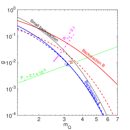
Figure 3: Consistency and backreaction constraints: Lower bound on $g$ from the requirement for ${\cal P}^{(v)}_{\zeta}$ to coincide with ${\cal P}^{obs}_{\zeta}$ (green line). Upper bound on $g$ from the requirement that the quantum loop corrections to the adiabatic curvature perturbations ${\cal R}_{\delta\phi}<0.1$ for $\epsilon_{QB}/\epsilon_{QE}<1$ (magenta continuous line ) and $\epsilon_{QB}/\epsilon_{QE}>1$ (magenta dashed line) with $r^{(v})=3.44\times 10^{-3}$ and $N_{k}=10$. Upper bound on $g$ required by the small backreaction regime (black dotted line). Upper bounds on $g$ from the full numerical computation including backreaction [62] for: i) the stable solution $m^{A}_{*}$ for $\lambda=100$ (continuous blue line) and $\lambda=50$ (dashed blue line) and ii) the stable solution $m^{B}_{*}$ for $\lambda=100$ (continuous red line) and $\lambda=50$ (dashed red line). The best fit solutions $m^{A}_{*}$ (blue star) and $m^{B}_{*}$ (red star) are also indicated.

4 Gravitational waves sourced by the axion-gauge field and Higgs portal interactions

In this section we provide constraints on the parameter space of the spectator axion-gauge field model in presence of Higgs portal interactions. For this purpose we take the Hubble expansion rate $H_{inf}$ during inflation at ${\phi_{*}}=5.26M_{pl}$, corresponding to the Hubble crossing of the largest observable CMB scale at $N\simeq 55$ e-folds before the end of inflation.

We evaluate the impact of Higgs portal interaction on parameters of the GW sourced tensor modes power spectrum $\{m_{*}\,,\epsilon^{*}_{B}\,,\sigma\,,r_{*}\}$ obtained for the stable solutions $m_{Q}$ given in Eq. (40) at their maximum values $m^{A}_{*}$ and $m^{B}_{*}$.
Figure 4 presents the evolution of these parameters with the Higgs-singlet quartic coupling $\lambda_{hs}$ for $\lambda_{s}=0.01$ and the spectator axion-gauge field model parameters $g\,,\lambda\,,\mu\,,f\,=\{10^{-2}\,,50\,,4\times 10^{-4}\,,10^{-2}\}$. All parameters show dependences on $\lambda_{hs}$ that are enhanced for the $m^{B}_{*}$ solution, with clear impact for the values of the sourced tensor-to-scalar ratio $r_{*}$. The figure shows that the Higgs portal interactions could enhance the GW signal sourced by the gauge field fluctuations in the CMB B-mode power spectra.

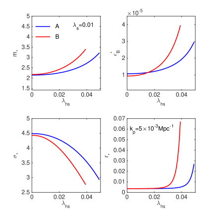
Figure 4: The evolution of $\{m_{*}\,,\epsilon^{*}_{B}\,,\sigma\,,r_{*}\}$ with the Higgs portal quartic coupling $\lambda_{hs}$ obtained for the stable solutions of $m_{Q}$ given in Eq. (40) at their maximum values $m^{A}_{*}$ (blue) and $m^{B}_{*}$ (red). The sourced tensor-to-scalar ratio $r_{*}$ is obtained at $k_{p}=5\times 10^{-3}$Mpc^-1. We take $\lambda_{s}=0.01$ and fix the axion-gauge field model parameters to: $g\,,\lambda\,,\mu\,,f\,=\{10^{-2}\,,50\,,4\times 10^{-4}\,,10^{-2}$}. The Hubble expansion rate during inflation is fixed at $\phi_{*}=5.26M_{pl}$ corresponding to the Hubble crossing of the largest observable CMB scale at $N\simeq 55$ e-folds before the end of inflation.

We perform an inference of the model parameters using the Monte-Carlo Markov Chains (MCMC) approach, accounting for consistency and backreaction constraints discussed in the previous section.
To obtain the variation intervals of the axion-gauge field parameters required by the MCMC analysis we use the confidence intervals of the Higgs-singlet inflation model given in Eq. (21).
The variation interval for the gauge coupling $g$ is obtained as follows: $g_{min}$ is calculated at $m_{*}=2.5$ from the requirement that ${\cal P}_{\zeta}$ should coincide with ${\cal P}^{obs}_{\zeta}$ as given by Eq. (44), while $g^{max}$ is obtained at $m_{*}=3.5$ from the requirement ${\cal R}_{\delta\phi}\leq 0.1$ using Eq. (45), as presented in Section 2.3.
The variation interval for the axion decay constant $f$ is obtained from the requirement $\kappa\lessgtr 1$, where $\kappa$ is given by Eq. (42), for $\lambda_{min}=30$ and $\lambda_{max}=100$.
The variation intervals for the modulation amplitude of the axion potential $\mu$ are calculated using the extrema values of $H_{inf}$ given in Eq. (21) and those of $g$, $f$, $\lambda$ and $m_{*}$ discussed above. We obtain these bounds for both $m^{A}_{Q}$ and $m^{B}_{Q}$ solutions. The intervals for axion-gauge field model parameters used in this analysis are given below:

$$g : \hskip 14.22636pt1.07\times 10^{-3}\,\,\,\div\,\,\,1.98\times 10^{-2}$$ (47)

$$f : \hskip 14.22636pt9.81\times 10^{-3}\,\,\,\div\,\,\,3.33\times 10^{-1}$$

$$\mu^{A} : \hskip 14.22636pt9.61\times 10^{-5}M_{pl}\,\,\,\div\,\,\,2.33\times 10^{-3}M_{pl}$$

$$\mu^{B} : \hskip 14.22636pt1.14\times 10^{-4}M_{pl}\,\,\,\div\,\,\,1.14\times 10^{-3}M_{pl}$$

$$\lambda : \hskip 14.22636pt30\,\,\,\div\,\,\,100$$

We modify the Boltzmann CAMB code [50] to compute $r_{*}$ and $\sigma$ given in Eq.(39) and to evaluate the sourced GW power spectra from Eq. (38) for the stable solutions $m^{A}_{*}$ and $m^{B}_{*}$, in the parameter intervals indicated in Eqs.(21) and (47). Our goal is to infer the axion-gauge field model parameter space for both solutions and to evaluate their impact on the CMB B-mode polarization power spectra.

To address the detectability of the GW sourced by the gauge field in presence of Higgs portal interactions we take as target model the Planck best fit $\Lambda$CDM model [8] with the vacuum tensor-to-scalar ratio $r^{(v)}=0.05$ at $k_{0}=0.05$Mpc^-1 and the normalisation $P^{obs}_{\zeta}=2.1\times 10^{9}$. We also take the noise power spectrum for the experimental configuration of the LiteBird mission given in Ref. [72].
As the sourced tensor modes are expected to exceed the vacuum contribution at large CMB observable scales, we take in this analysis the B-modes polarization power spectra in the multipole interval ${\it l}\simeq(2\,\,\div\,\,150)$ and evaluate the GW sourced tensor-to-scalar ratio at $k_{p}=5\times 10^{-3}$. As before, we use the Monte-Carlo Markov Chains (MCMC) technique to sample from the space of axion-gauge field and Higgs portal parameters and generate estimates of their posterior distributions. As mentioned, we assume a flat universe and uniform priors for all parameters adopted in the analysis.
Left panel from Figure 5 presents the best fit sourced GW power spectra for $m^{A}_{*}$ and $m^{B}_{*}$ solutions, while right panel from the same figure shows the corresponding B-mode polarization power spectra. For comparison, the B-mode polarization power spectra of $\Lambda$CDM target model and Higgs-singlet inflation model are also presented.

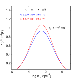
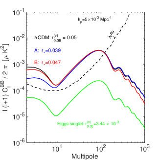
Figure 5: Left: The best fit of sourced GW power spectra ${\cal P}^{(s)}_{t}$ for $m^{A}_{*}$ (blue line) and $m^{B}_{*}$ (red line) solutions. The best fit parameters of ${\cal P}^{(s)}_{t}$ are also indicated. Right: The corresponding best fit B-mode polarization power spectra for $m^{A}_{*}$ (blue line) and $m^{B}_{*}$ (red line) solutions. For comparison, the B-mode polarization power spectra of $\Lambda$CDM target model (black line) and Higgs-singlet inflation model (green line) are presented.The noise power spectrum $N^{BB}_{l}$ (black dashed line) corresponding to the LiteBird mission experimental configuration [72] is also shown. .

The spectrum of the sourced GW energy density at the present time and at a given frequency $f=k/2\pi$ can be approximated as [63]:

$$h^{2}\Omega_{GW}(f)=\frac{3}{128}\Omega_{rad}{\cal P}^{(s)}_{t}(f)\left[\frac{1}{2}\left(\frac{f_{eq}}{f}\right)^{2}+\frac{16}{9}\right]\,,$$ (48)

where $h^{2}$ is defined such that $H_{0}=100h$ km s^-1 Mpc^-1 is the Hubble parameter at the present time, ${\cal P}^{(s)}_{t}(f)$ is power spectrum of the sourced tensor modes, $\Omega_{rad}=(1-f_{\nu})^{-1}\Omega_{\gamma}$ is the present radiation energy density parameter, $(1-f_{\nu})^{-1}=1.68$ for the SM expectation value of $N_{eff}=3.046$ relativistic degrees of freedom [64], $\Omega_{\gamma}=2.38\times 10^{-5}h^{-2}$ is the present photon energy density parameter and $f_{eq}=1.09\times 10^{-17}$ Hz is the frequency entering the horizon at matter-radiation equality. We use $f/Hz=1.5\times 10^{-15}k/Mpc^{-1}$ .
Left panel from Figure 6 presents the evolution with frequency of the energy density parameter $h^{2}\Omega_{GW}(f)$ of the sourced primordial GW for $m^{A}_{*}$ and $m^{B}_{*}$ best fit solutions obtained for the LiteBird observing strategy. The solid green line shows the vacuum energy contribution of Higgs-singlet model. In all cases the GW energy density spectrum at present time is adiabatic with a slope that change at frequency scales that make the transition between matter and radiation domination eras.
For comparison we also show $h^{2}\Omega_{GW}(f)$ sourced by axion-SU(2) gauge field model AX2 from Ref. [69]. For all cases the GW energy spectra are adiabatic with a slope that change at frequency scales corresponding to modes entering the horizon during the matter-radiation equality.
In the right panel from Figure 6 we show the same $h^{2}\Omega_{GW}(f)$ power spectra along with the sensitivity curves of the future satellite-borne GW interferometers LISA [65], DECIGO [66] and BBO [67]. As $h^{2}\Omega_{GW}(f)$ power spectra covers 55 e-folds before the end of inflation, to provide a comparison with the sensitivity of LISA, DECIGO and BBO, we rescale the GW frequency to 15 e-folds before the end of inflation [61].
The sensitivity curves of the GW interferometers are obtained by using the ‘strain noise power spectra” file available online in Zenodo repository [42, 68]. The $h^{2}\Omega_{GW}(f)$ power spectra obtained for $m^{A}_{*}$ and $m^{B}_{*}$ best fit solutions obtained for the LiteBird observing strategy are potentially detectable in the frequency rage $10^{-2}$Hz - 1 Hz.

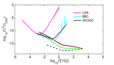
Figure 6: Left: Evolution with frequency of the energy density parameter $h^{2}\Omega_{GW}(f)$ of the sourced primordial GW for $m^{A}_{*}$ (blue line) and $m^{B}_{*}$ (red line) best fit solutions obtained for the LiteBird observing strategy. The solid green line shows the vacuum energy contribution of Higgs-singlet model. In all cases the GW energy density spectra at present time are adiabatic with a slope that change at frequency scales that make the transition between matter and radiation domination eras. For comparison we also show $h^{2}\Omega_{GW}(f)$ sourced by axion-SU(2) gauge field model AX2 from Ref. [69]. Right: The $h^{2}\Omega_{GW}(f)$ power spectra presented in the left panel, rescaled at GW frequencies corresponding to 15 e-folds before the end of inflation, and the sensitivity curves for LISA, DECIGO, and BBO interferometers.

Table 1 presents the mean values and absolute errors at 68% confidence of the model parameters obtained from the MCMC analysis for $m^{A}_{*}$ and $m^{B}_{*}$ solution. We find that the tensor-to-scalar ratio of the sourced GW in presence of Higgs portal interactions is enhanced to a level that overcomes the vacuum tensor-to-scalar ratio by a factor ${\mathcal{O}}$(10) for both solutions, much above the detection threshold of the near-future B-modes polarization LiteBird experiment, in agreement with the CMB observations on curvature fluctuations and with the allowed parameter space of Higgs portal interactions.

In Figure 7 and Figure 8 we present the marginalised probability distributions of the axion-gauge field spectator model with Higgs portal interactions for the $m^{A}_{*}$ and $m^{B}_{*}$ solutions. The figures show the correlation between axion-gauge field model parameters $\{g,\,\lambda,\,\mu,\,f\}$ and the power spectrum of the sourced tensor modes parameters $\{r_{*},\,\sigma,\,m_{*}\}$ at $k_{p}=5\times 10^{-3}$Mpc^-1.

Figure 7: The marginalised probability distributions obtained for the parameters of the axion-gauge field spectator model with Higgs portal interactions for $m^{A}_{*}$ solution at $k_{p}\leavevmode\nobreak\ =\leavevmode\nobreak\ 5\leavevmode\nobreak\ \times\leavevmode\nobreak\ 10^{-3}$ Mpc ^-1.

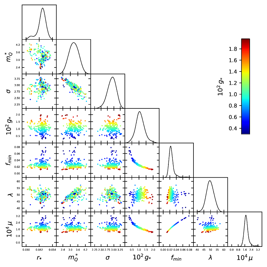
Figure 8: The marginalised probability distributions obtained for the parameters of the axion-gauge field spectator model with Higgs portal interactions for $m^{B}_{*}$ solution at $k_{p}\leavevmode\nobreak\ =\leavevmode\nobreak\ 5\leavevmode\nobreak\ \times\leavevmode\nobreak\ 10^{-3}$ Mpc ^-1.

Figure 9 presents the 2D marginalised probability distributions in $m_{*}\leavevmode\nobreak\ -\leavevmode\nobreak\ \delta\lambda_{h}$ plane for $m^{A}_{*}$ (blue) and $m^{B}_{*}$ (red) solutions at 68% and 95% confidence intervals. The figure shows the correlations between $m_{*}$ and the threshold correction of the Higgs quartic coupling $\delta\lambda_{h}=\lambda^{2}_{hs}/4\lambda_{s}$.

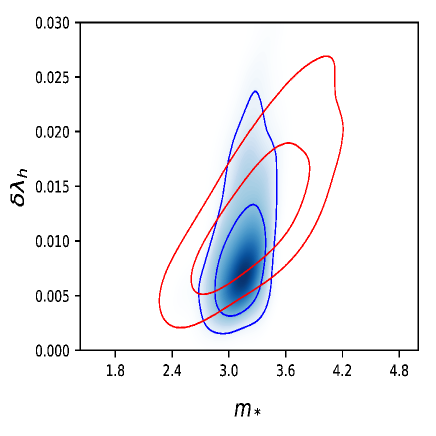
Figure 9: The 2D marginalised probability distributions obtained for $m^{A}_{*}$ (blue) and $m^{B}_{*}$ (red) solutions at 68% and 95% confidence intervals. The figure shows the correlations between $m_{*}$ and the threshold correction of the Higgs quartic coupling $\delta\lambda_{h}=\lambda^{2}_{hs}/4\lambda_{s}$.

Table 1: The mean values and absolute errors of the parameters of the axion-gauge field spectator model with Higgs portal interactions obtained at $k_{p}\leavevmode\nobreak\ =\leavevmode\nobreak\ 5\leavevmode\nobreak\ \times\leavevmode\nobreak\ 10^{-3}$ Mpc ^-1 for $m^{A}_{*}$ and $m^{B}_{*}$ solutions. The errors are quoted at 68% CL.

Parameter	$m^{A}_{*}$	$m^{B}_{*}$
$r_{*}$	0.039 $\pm$ 0.0027	0.047 $\pm$ 0.0031
$m_{*}$	3.091 $\pm$ 0.035	3.201 $\pm$ 0.036
$\sigma$	3.061 $\pm$ 0.185	2.940 $\pm$0.164
$g$	$(8.32\pm 0.048)\times 10^{-3}$	(1.01 $\pm$ 0.03) $\times 10^{-2}$
$\lambda$	50.85$\pm$ 1.34	49.46 $\pm$1.49
$\mu$	(6.21 $\pm$ 0.12) $\times 10^{-4}$	(2.15 $\pm$ 0.28) $\times 10^{-4}$
$f$	(4.37 $\pm$ 0.31)$\times 10^{-2}$	(2.15 $\pm$ 0.17) $\times 10^{-2}$
$\lambda_{s}$	0.084 $\pm$ 0.011	0.071 $\pm$ 0.022
$\lambda_{hs}$	0.049 $\pm$ 0.002	0.051 $\pm$ 0.001
$\delta_{\lambda_{h}}$	(7.11 $\pm$ 0.021) $\times 10^{-3}$	(1.18 $\pm$0.03) $\times 10^{-2}$

5 Conclusions

In this work we investigate a scenario where an axion field and an non-Abelian gauge field are confined to the spectator sector while the inflation sector is represented by a mixture of Higgs boson and a scalar singlet with large non-zero vev that are non-minimally coupled to gravity. We assume that there is no coupling, up to gravitational interactions, between inflation and spectator sectors, the background energy density is dominated by the inflaton and the Hubble expansion is constant during inflation.

We place constraints on Higgs-singlet model parameters from the requirement to satisfy the observational bounds on the curvature perturbations. We show that a mixture of Higgs boson with a heavy scalar singlet with large vev is a viable model of inflation that satisfy the existing observational data and the perturbativity constraints, avoiding at the same time the EW vacuum metastability as long as the Higgs portal interactions lead to positive tree-level threshold corrections for SM Higgs quartic coupling.

We evaluate the impact of the Higgs quartic coupling threshold corrections on the GW sourced tensor modes power spectrum for two stable slow-roll solutions for the mass parameter of gauge field fluctuations [62] while accounting for the consistency and backreaction constraints.
We show that the Higgs portal interactions enhance the GW signal sourced by the gauge field fluctuations in the CMB B-mode ploarization power spectra.

To address the detectability of the GW sourced by the gauge field fluctuations in presence of Higgs portal interactions we take as target model the Planck best fit $\Lambda$CDM cosmology [7, 8] with the vacuum tensor-to-scalar ratio $r^{(v)}=0.05$ at $k_{0}=0.05$Mpc^-1 and the noise power spectrum for the experimental configuration of the LiteBird mission [72]. Using the MCMC technique we sample from the parameter spaces of Higgs-singlet and axion-gauge field model and generate estimates of model parameters from their posterior distributions. We obtain in this way comprehensive constrains on Higgs portal, axion-gauge field and sourced GW power spectra parameters.

We find that the tensor-to-scalar ratio of the sourced GW in presence of Higgs portal interactions is enhanced to a level that overcomes the vacuum tensor-to-scalar ratio by a factor $\mathcal{O}$(10), much above the detection threshold of the near-future B-modes polarization LiteBird experiment, in agreement with the CMB observations on curvature fluctuations and with the allowed parameter space of Higgs portal interactions.

A large enhancement of the GW sourced can be also detected by experiments such as pulsar timing arrays and laser/atomic interferometers [72, 69].
On the other hand, a significant Higgs-singlet mixing can be probed at LHC by the measurement of production cross sections for Higgs-like states [45, 37], while a significant tree level threshold of the Higgs quartic coupling can be measured at colliders [27, 28].

6 Acknowledgment

The author acknowledges the use of the GRID computing facility at the Institute of Space Science.
This research was supported by the Romanian Ministry of Research, Innovation and Digitalization under the Romanian National Core Program LAPLAS VII - contract no. 30N/2023.

7 References

References

- [1] A. H. Guth, Inflationary universe: A possible solution to the horizon and flatness problems, Phys. Rev. D 23 (1981) 347.
- [2] A. D. Linde, A new inflationary universe scenario: A possible solution of the horizon, flatness, homogeneity, isotropy and primordial monopole problems, Phys. Lett. B 108 (1982) 389-393.
- [3] A. Albrecht and P. J. Steinhardt, Cosmology for Grand Unified Theories with Radiatively Induced Symmetry Breaking, Phys. Rev. Lett. 48 (1982) 1220.
- [4] V. F. Mukhanov and G. V. Chibisov, Quantum Fluctuations and a Nonsingular Universe, JETP Lett. 33 (1981) 532.
- [5] A. A. Starobinsky, Dynamics of phase transition in the new inflationary universe scenario and generation of perturbations, Phys. Lett. B 117 (1982) 175.
- [6] J. M. Bardeen, P. J. Steinhardt and M. S. Turner, Spontaneous creation of almost scale-free density perturbations in an inflationary universe, Phys. Rev. D 28 (1983) 679.
- [7] Planck Collaboration: Y. Akrami et al., Planck 2018 results X. Constraints on inflation, Astron. Astrophys. 641 (2020) A10 [1807.06211].
- [8] Planck Collaboration: N. Aghanim et al., Planck 2018 results. VI. Cosmological parameters, Astron. Astrophys. 641 (2020) A6 [1807.06209].
- [9] P. A. R Ade et al., Improved Constraints on Primordial Gravitational Waves using Planck, WMAP, and BICEP/Keck Observations through the 2018 Observing Season, PRL 127 (2021) 15, 151301 [2110.00483].
- [10] M. Hazumi et al., LiteBIRD: A Satellite for the Studies of B-Mode Polarization and Inflation from Cosmic Background Radiation Detection, J. Low Temp. Phys. 194 (2019) 443.
- [11] LiteBIRD Collaboration ; E. Allys et al., E. Probing cosmic inflation with the LiteBIRD cosmic microwave background polarization survey, Progress of Theoretical and Experimental Physics 4 (2023) 143 [2202.02773].
- [12] CMB-S4 collaboration, K. Abazajian et al., CMB-S4 Science Book, First Edition [1610.02743].
- [13] L.P. Grishchuk, Amplification of gravitational waves in an istropic universe, Zh. Eksp. Teor. Fiz. 67 (1974) 825.
- [14] A.A. Starobinsky, Spectrum of relict gravitational radiation and the early state of the universe, JETP Lett. 30 (1979) 682.
- [15] D.H. Lyth, What would we learn by detecting a gravitational wave signal in the cosmic microwave background anisotropy?, Phys. Rev. Lett. 78 (1997) 1861 [9606387].
- [16] P. Adshead and M. Wyman, Natural Inflation on a Steep Potential with Classical Non- Abelian Gauge Fields, Phys. Rev. Lett. 108 (2012) 261302 [1202.2366].
- [17] P. Adshead and M. Wyman, Gauge-inflation trajectories in chromo-natural inflation, Phys. Rev. D 86 (2012) 043530 [1203.2264].
- [18] N. Barnaby and M. Peloso, Large Nongaussianity in Axion Inflation, Phys. Rev. Lett. 106 (2011) 181301 [1011.1500].
- [19] J.L. Cook and L. Sorbo, An inflationary model with small scalar and large tensor nongaussianities, JCAP 11 (2013) 047 [1307.7077].
- [20] O. Ozsoy, Parity violating non-Gaussianity from axion-gauge field dynamics, Phys. Rev. D 104 (2021) 123523 [2106.14895].
- [21] A. Agrawal, T. Fujita and E. Komatsu, Large tensor non-Gaussianity from axion-gauge field dynamics, Phys. Rev. D 97 (2018) 103526 [1707.03023].
- [22] A. Agrawal, T. Fujita and E. Komatsu, Tensor Non-Gaussianity from Axion-Gauge-Fields Dynamics : Parameter Search, JCAP 06 (2018) 027 [1802.09284].
- [23] M. Shiraishi, C. Hikage, R. Namba, T. Namikawa and M. Hazumi, Testing statistics of the CMB B -mode polarization toward unambiguously establishing quantum fluctuation of the vacuum, Phys. Rev. D 94 (2016) 043506 [1606.06082].
- [24] A. Lue, L.-M. Wang and M. Kamionkowski, Cosmological signature of new parity violating interactions, Phys. Rev. Lett. 83 (1999) 1506 [astro-ph/9812088].
- [25] R. Namba, E. Dimastrogiovanni and M. Peloso, Gauge-flation confronted with Planck, JCAP 11, 045 (2013) [arXiv:1308.1366]
- [26] E. Pajer and Marco Peloso, A review of axion inflation in the era of Planck, Class. Quantum Grav. 30 (2013) 214002 [1305.3557]
- [27] ATLAS Collaboration Collaboration, G. Aad et al., Observation of a new particle in the search for the Standard Model Higgs boson with the ATLAS detector at the LHC, Phys.Lett. B716 (2012) 1 [1207.7214].
- [28] CMS Collaboration Collaboration, S. Chatrchyan et al., Observation of a new boson at a mass of 125 GeV with the CMS experiment at the LHC, Phys.Lett. B 716 (2012) 30 [207.7235].
- [29] J. Beacham, et al., Physics Beyond Colliders at CERN Beyond the Standard Model Working Group Report, J. Phys. G 47 (2020) 1, 010501 [arXiv:1901.09966]
- [30] F. L. Bezrukov and M. Shaposhnikov, Phys. Lett. B 659, 703 (2008).
- [31] F. Bezrukov, A. Magnin, M. Shaposhnikov and S. Sibiryakov, Higgs inflation: consistency and generalisations, JHEP 1101 (2011) 016 [1008.5157]
- [32] F. Bezrukov, J. Rubio and M. Shaposhnikov, Living beyond the edge: Higgs inflation and vacuum metastability Phys. Rev. D 92 (2015) 083512 [1412.3811].
- [33] G. Degrassi, S. Di Vita, J. Elias-Miro, J. R. Espinosa, G. F. Giudice, G. Isidori and A. Strumia, Higgs mass and vacuum stability in the Standard Model at NNLO, JHEP 1208 (2012) 098 [1205.6497 ].
- [34] O. Lebedev and H. M. Lee, The Higgs portal interactions, Eur. Phys. J. C 71 (2011) 1821.
- [35] J. Elias, J. R. Espinosa, G. F. Giudice, H. M. Lee, A. Strumia, Stabilization of the Electroweak Vacuum by a Scalar Threshold Effect, JHEP 2012 (2012) 31 [1203.0237].
- [36] T. Robens, T. Stefaniak, LHC benchmark scenarios for the real Higgs singlet extension of the standard model, Eur. Phys. Jour. C76 (2016) 268 [1601.07880].
- [37] S. Navas et al. (Particle Data Group), Phys. Rev. D 110, 030001 (2024).
- [38] O. Lebedev,The Higgs Portal to Cosmology, Progress in Particle and Nuclear Physics 120 (2021) 103881 [ arXiv:2104.03342].
- [39] C. Caprini, M. Hindmarsh, S. Huber et al, Science with the space-based interferometer eLISA. II: gravitational waves from cosmological phase transitions, JCAP 04 (2016) 001 [1512.06239].
- [40] V. K. Oikonomou, A. Giovanakis, Electroweak phase transition in singlet extensions of the standard model with dimension-six operators, Phys. Rev. D109 (2024) 055044 [ arXiv:2403.01591].
- [41] T. Alanne, T. Hugle, M. Platscher, K. Schmitz, A fresh look at the gravitational-wave signal from cosmological phase transitions, JHEP 03 (2020) 4 [1909.11356].
- [42] K. Schmitz, New Sensitivity Curves for Gravitational-Wave Signals from Cosmological Phase Transitions, JHEP 01 (2021) 097 [2002.04615].
- [43] V. K. Oikonomou, Effects of the axion through the Higgs portal on primordial gravitational waves during the electroweak breaking, Phys. Rev. D110 (2023) 075003 [2303.05889]
- [44] V. K. Oikonomou, Theoretical probes of Higgs boson-axion nonperturbative couplings, Phys. Rev. D110 (2024) 075003 [2409.10709]
- [45] A.Falkowski, C. Gross, O. Lebedev, A second Higgs from the Higgs portal, JHEP 2015 (2015) 57 [1502.01361]
- [46] Y. Ema, Higgs scalaron mixed inflation, Phys. Lett. B, (2017) 770, 403 [1701.07665].
- [47] Y. Ema, M. Karciauskas, O. Lebedev, S. Rusak and M. Zatta, Higgs inflaton mixing and vacuum stability, Phys. Lett. B 789 (2019) 373 [1711.10554].
- [48] J. Kim, P. Ko, W. Park, Higgs-portal assisted Higgs inflation with a sizeable tensor-to-scalar ratio, JCAP 02 (2017) 003 (2017) [1405.1635].
- [49] R. N. Lerner and J. McDonald, Gauge singlet scalar as inflaton and thermal relic dark matter, Phys. Rev. D 80 (2009) 123507 [0909.0520].
- [50] A. Lewis, A. Challinor, A. Lasenby, Efficient computation of CMB anisotropies in closed FRW models, ApJ 538 (2000) 473.
- [51] P. Adshead and M. Wyman, Chromo-Natural Inflation: Natural inflation on a steep potential with classical non-Abelian gauge fields, Phys. Rev. Lett. 108 (2012) 261302 [1202.2366].
- [52] P. Adshead, E. Martinec and M. Wyman, Gauge fields and inflation: Chiral gravitational waves, fluctuations, and the Lyth bound, Phys. Rev. D 88 (2013) 021302 [1301.2598].
- [53] P. Adshead, E. Martinec, E.I. Sfakianakis and M. Wyman, Higgsed Chromo-Natural Inflation, JHEP 12 (2016) 137 [1609.04025].
- [54] E. Dimastrogiovanni, M. Fasiello and T. Fujita, Primordial Gravitational Waves from Axion-Gauge Fields Dynamics, JCAP 01 (2017) 019 [1608.04216].
- [55] N. Barnaby, J. Moxon, R. Namba, M. Peloso, G. Shiu et al., Gravity waves and non-Gaussian features from particle production in a sector gravitationally coupled to the inflaton, Phys.Rev. D 86 (2012) 103508 [1206.6117].
- [56] R. Namba, M. Peloso, M. Shiraishi, L. Sorbo and C. Unal, Scale-dependent gravitational waves from a rolling axion, JCAP 1601 (2016) 041 [1509.07521].
- [57] O. Ozsoy, Synthetic Gravitational Waves from a Rolling Axion Monodromy, JCAP 04 (2021) 040 [2005.10280].
- [58] A. Maleknejad and M.M. Sheikh-Jabbari, Gauge-flation: Inflation From Non-Abelian Gauge Fields, (2011) [arXiv:1102.1513].
- [59] A. Maleknejad and M.M. Sheikh-Jabbari, Non-Abelian gauge field inflation, Phys. Rev. D 84 (2011) 043515 [1102.1932]
- [60] D. I. Kaiser, Conformal Transformations with Multiple Scalar Fields, Phys. Rev. D, 81 (2010) 084044 [1003.1159].
- [61] O. Iarygina, E. Sfakianakis, R. Sharma, A. Brandenburg, Backreaction of axion-SU(2) dynamics during inflation, JCAP 04 (2024) 18, 28 [2311.07557].
- [62] K. Ishiwata, E. Komatsu, I. Obata, Axion-gauge field dynamics with backreaction, JCAP 03 (2022) 03, 10 [2111.14429].
- [63] C. Caprini and D.G. Figueroa, Cosmological Backgrounds of Gravitational Waves, Class. Quant. Grav. 35 (2018) 163001 [1801.04268].
- [64] P. F. de Salas, S. Pastor, Relic neutrino decoupling with flavour oscillations revisited, JCAP 07 (2016) 051 [1606.06986 ]
- [65] LISA Collaboration, H. Audley et al., Laser Interferometer Space Antenna, [1702.00786].
- [66] S. Isoyama, H. Nakano, and T. Nakamura, Multiband Gravitational-Wave Astronomy: Observing binary inspirals with a decihertz detector, B-DECIGO, PTEP 2018 (2018) 073E01 [1802.06977].
- [67] V. Corbin and N. J. Cornish, Detecting the cosmic gravitational wave background with the big bang observer, Class. Quant. Grav. 23 (2006) 2435 [0512039].
- [68] K. Schmitz, New Sensitivity Curves for Gravitational-Wave Experiments, https://zendo.org/records/368958 (2020).
- [69] P. Campeti, E. Komatsu, D. Poletti, C. Baccigalupi, Measuring the spectrum of primordial gravitational waves with CMB, PTA and Laser Interferometers. JCAP 01 (2021) 012 [2007.04241].
- [70] A. Papageorgiou, M. Peloso and C. Unal, Nonlinear perturbations from axion-gauge fields dynamics during inflation, JCAP 07 (2019) 004, [1904.01488].
- [71] T. Fujita, R. Namba, Y. Tada, Does the detection of primordial gravitational waves exclude low energy inflation?, Physics Lett B, 778 (2018) 17 [1705.01533]
- [72] B. Thorne, T. Fujita, M. Hazumi, N. Katayama, E. Komatsu, M. Maresuke, Finding the chiral gravitational wave background of an axion-S U (2 ) inflationary model using CMB observations and laser interferometers, Phys. Rev. D 97 (2018) 043506 [1707.03240].
- [73] P., Campeti, E. Komatsu, C. Baccigalupi et al., LiteBIRD science goals and forecasts. A case study of the origin of primordial gravitational waves using large-scale CMB polarization, JCAP 06, (2024) 008.
- [74] E. Dimastrogiovanni and M. Peloso, Stability analysis of chromo-natural inflation and possible evasion of Lyth bound, Phys. Rev. D 87 (2013) 103501 [1212.5184].
- [75] T. Fujita, E. Sfakianakis, M. Shiraishi,Tensor Spectra Templates for Axion-Gauge Fields Dynamics during Inflation, JCAP 05 (2019) 057 [1812.03667].
- [76] P. Campeti, E. Komatsu, C. Baccigalupi et al., LiteBIRD science goals and forecasts. A case study of the origin of primordial gravitational waves using large-scale CMB polarization, JCAP 06 (2024) 008 [2312.00717].
- [77] A. Papageorgiou, M. Peloso, C. Unal, Nonlinear perturbations from the coupling of the inflaton to a non-Abelian gauge ?field, with a focus on Chromo-Natural Inflation, JCAP 09 (2018) 030 [ arXiv:1806.08313
- [78] T. Fujita, R. Namba, I. Obata, Mixed non-gaussianity from axion-gauge field dynamics, JCAP 04 (2019) 044 [1811.12371].
- [79] A. Maleknejad and E. Komatsu, Production and Backreaction of Spin-2 Particles of SU(2) Gauge Field during Inflation, JHEP 05 (2019) 174 [1808.09076].
- [80] L. Mirzagholi, A. Maleknejad and K.D. Lozanov, Production and backreaction of fermions from axion-SU(2) gauge fields during inflation, Phys. Rev. D 101 (2020) 083528 [1905.09258].