Mapping reionization bubbles in the JWST era II:
inferring the position and characteristic size of individual bubbles
The James Webb Space Telescope (JWST) is discovering an increasing number of galaxies well into the early stages of the Epoch of Reionization (EoR). Many of these galaxies are clustered with strong Lyman alpha (Ly) emission, motivating the presence of surrounding cosmic HII regions that would facilitate Ly transmission through the intergalactic medium (IGM). Detecting these HII ”bubbles” would allow us to connect their growth to the properties of the galaxies inside them. Here we develop a new forward-modeling framework to estimate the local HII region size and location from Ly spectra of galaxy groups in the early stages of the EoR. Our model takes advantage of the complementary information provided by neighboring sightlines through the IGM. Our forward models sample the main sources of uncertainty, including: (i) the global neutral fraction; (ii) EoR morphology; (iii) emergent Ly emission; and (iv) NIRSpec instrument noise. Depending on the availability of complementary nebular lines, 0.006 – 0.01 galaxies per cMpc3, are required to be 95% confident that the HII bubble location and size recovered by our method is accurate to within 1 comoving Mpc. This corresponds roughly to tens of galaxies at –8 in 2x2 tiled pointing with JWST NIRSpec. Such a sample is achievable with a targeted survey with completeness down to -19 – -17, depending on the over-density of the field. We test our method on 3D EoR simulations as well as misspecified equivalent width distributions, in both cases accurately recovering the HII region surrounding targeted galaxy groups.
Key Words.:
Galaxies: high-redshift – intergalactic medium – Cosmology: dark ages, reionization, first stars1 Introduction
The Epoch of Reionization (EoR) marks an important milestone in the Universe’s evolution. UV radiation from the first, clustered galaxies reionized their surrounding intergalactic medium (IGM). These HII ”bubbles” expanded, percolated, and eventually permeated all of space, completing the final phase change of our Universe. The timing and morphology of the EoR tell us which galaxies were responsible as well the role of IGM clumps that regulated the end stages (e.g., McQuinn et al., 2007; Sobacchi & Mesinger, 2014).
Lyman emission from galaxies is an especially useful tool for studying the early stages of the EoR, when HII regions are relatively small such that the neutral IGM leaves a strong imprint via damping wing absorption (e.g., see review in Dijkstra, 2014). A common approach is to estimate the mean neutral fraction of the IGM using a statistically large sample of galaxies (e.g., Mesinger & Furlanetto 2008b; Stark et al. 2010; Mesinger et al. 2015; Mason et al. 2018; Jung et al. 2020; Bolan et al. 2022; Jones et al. 2024; Nakane et al. 2024). However, galaxies reside in biased regions of the IGM, and connecting the corresponding damping wing signature to the mean neutral fraction is very model dependent (e.g., Mesinger & Furlanetto, 2008a; Lu et al., 2024a). In contrast, unbiased probes such as the Lyman alpha forest are sourced from representatively-large volumes of the IGM, and can already tightly constrain the mean neutral fraction during the latter half of the EoR (Qin et al., 2021; Bosman et al., 2022; Qin et al., 2024).
In addition to estimating the global neutral fraction from the IGM Ly damping wings, one could instead infer the presence (or lack thereof) of an individual HII region surrounding an observed group of galaxies (Tilvi et al., 2020; Endsley & Stark, 2022; Jung et al., 2022; Hayes & Scarlata, 2023). This could potentially allow us to connect the growth of the local HII region to the properties of the galaxies inside it. Having several such estimates of HII bubble sizes will allow us to understand which kind of galaxies drove reionization (e.g., faint/bright; McQuinn et al., 2007; Mesinger et al., 2016), well before the advent of tomographic 21cm maps with the Square Kilometer Array (SKA). Fortunately, the James Webb Space Telescope (JWST) is providing spectra from an ever-increasing number of galaxy groups at high redshifts which can be used for this purpose (e.g., Saxena et al., 2023; Witstok et al., 2024a; Tang et al., 2023, 2024b; Chen et al., 2024; Umeda et al., 2024; Napolitano et al., 2024)
However, the interpretation of these observations has so far been fairly approximate. The presence of an IGM damping wing in each galaxy is estimated independently of its neighbors. This wastes invaluable information, as neighboring galaxies provide complimentary sightlines into the local EoR morphology. The result is that the studies focusing on individual galaxies generally only predict lower limits for the radii of local HII regions. Furthermore, studies tend to ignore one or more important sources of stochasticity in the EoR morphology, intrinsic galaxy emission and/or telescope noise.
In this work we develop a new framework to infer the local HII region size and location from Ly observations of a galaxy group. Our formalism accounts for the relative position of each galaxy with respect to the host and nearby HII bubbles by creating self-consistent forward models of JWST/NIRSpec spectra for each galaxy. We account for the relevant sources of uncertainty/stochasticity, including: (i) the IGM mean neutral fraction, ; (ii) the EoR morphology, given ; (iii) the emergent Ly emission, given the observed UV magnitudes; and (iv) NIRSpec instrument noise. Unlike many previous studies, we do not make any assumptions about the unknown relative contribution of observed versus unobserved galaxies to the growth of the local HII region. We quantify how many galaxies are required to robustly detect individual ionized regions with a accuracy in their inferred location and characteristic size, during the early stages of EoR. This work is a companion to Lu et al. (2024b), in which we presented a complementary formalism to detect edges of ionized regions, using empirically-calibrated relations.
This paper is structured as follows. In Section 2 we present our forward modeling pipeline for Ly galaxy spectra during the EoR. We introduce our procedure to infer the size and location of the surrounding HII region in Section 3. We apply our framework to mock data and show our main results in Section 4. We build further confidence by performing out-of-distribution tests in Section 5. In Section 6 we quantify observational requirements for detecting individual HII regions and we conclude in Section 7. All quantities are presented in comoving units unless stated otherwise. We assume a standard CDM cosmology (), with parameters consistent with the latest estimates from Planck Collaboration et al. (2020). All quantities are quoted in comoving units and evaluated in the rest-frame, unless stated otherwise.
2 Observing Lyman alpha spectra from galaxies during the EoR
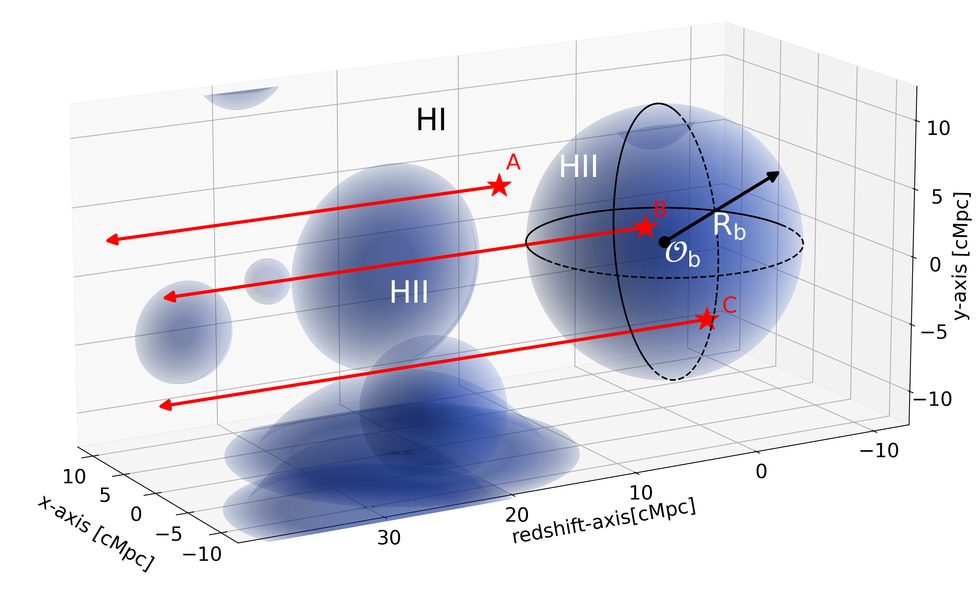
Our fiducial set-up is shown in Fig. 1. An HII region in an observed galaxy field is characterized as a sphere, with a center location () and characteristic radius (). This is the ”local” or ”target” HII region whose properties we aim to infer. Nearby ionized regions are also shown in blue in the diagram. Observed galaxies can be located both inside and outside HII regions; here we denote three such galaxies with ’A’, ’B’, ’C’, highlighting their sightlines towards the observer with red arrows.
Specifically, we wish to determine the conditional probability of the HII bubble center, , and radius, , given observed Ly spectra of galaxies in a field with a central redshift ,
| (1) |
Here , , and are vectors of the galaxies’ Cartesian coordinates, UV magnitudes, and observed Ly spectra. For each galaxy, the observed spectrum in the rest-frame can be written as:
| (2) |
where is the emergent111Throughout we use the term ”emergent” to refer to values escaping from the galaxy into the IGM. Therefore the emergent amplitude, , and profile, , are determined by Lyman alpha radiative transfer through the interstellar medium (ISM) and the circumgalactic medium (CGM; e.g. Neufeld 1990; Laursen et al. 2011). We do not model the details of this radiative transfer in this work, but instead rely on empirical relations based on post-EoR observations to determine the conditional distributions of and . Lyman-alpha luminosity of a galaxy, is the normalized, emergent Lyman- profile, accounts for IGM attenuation, and is the spectrograph noise.
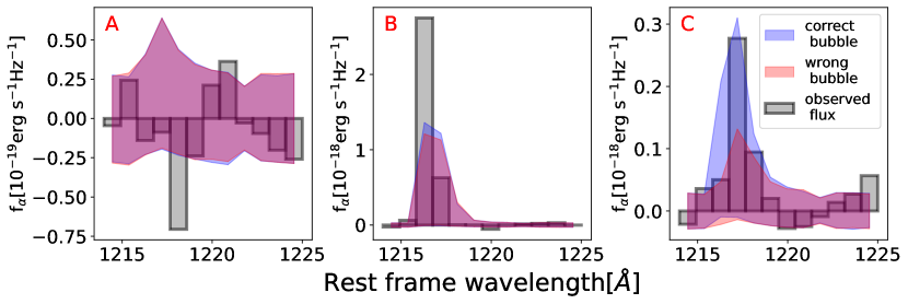
In the schematic shown in Fig. 1, galaxy ’A’ is outside of an ionized bubble, and its Lyman flux will therefore be strongly attenuated by the neutral IGM (i.e. having a large ). We should only detect Lyman alpha flux from galaxy ’A’ if it has a high emergent luminosity, , and its Ly profile, , is strongly redshifted from the systemic (e.g., Dijkstra 2014). Galaxy ’B’ is close to the center of the local HII bubble, and will have (on average; c.f. right panel of Fig. 5), the lowest Ly damping wing attenuation from the patchy EoR. However, the observed flux depends on all of the terms in eq. (2), each of which can have sizable stochasticity. Below we detail how each of these terms.
2.1 emergent Lyman-alpha profile
We start with the Lyman-alpha profile emerging into the IGM, , normalized to integrate to unity. In order to escape the ISM of the galaxy, Lyman- photons must diffuse spectrally which leads to a double-peaked Lyman-alpha shape (Neufeld, 1990; Hu et al., 2023; Hutter et al., 2023; Almada Monter & Gronke, 2024). Due to the resonant nature of the line, the blue peak generally gets absorbed even by the ionized IGM at (though see Meyer et al. 2021 for some putative, rare counter examples). Following Mason et al. (2018), we model the remaining red peak as a Gaussian:
| (3) |
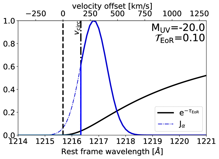
where represents the velocity offset from systemic of the center of the line, and is the velocity difference from the resonant wavelength of the line, . As in Mason et al. (2018), for simplicity we assume that the FWHM of the line is equal to the velocity of the offset (e.g., Verhamme et al., 2018). Although these profiles are motivated by lower redshift observations (e.g. Yamada et al. 2012; Orlitová et al. 2018; Hu et al. 2023), we note that our framework can easily accommodate any distribution for , once we have better models for the emergent spectra. We also assume that all Lyman-alpha photons with a velocity offset below the circular velocity, , of the host halo are absorbed by the CGM (Dijkstra et al., 2011; Laursen et al., 2011). In Fig. 2 we show an example of the emergent profile in blue, for a galaxy with UV magnitude and velocity offset km/s, with a km/s.
The PDF of the emergent velocity offset is well described by a log-normal distribution (Steidel et al., 2014; De Barros et al., 2017; Stark et al., 2017; Mason et al., 2018):
| (4) |
where the mean velocity offset is correlated with the UV magnitude (Stark et al., 2017, though see Bolan et al. (2024)):
| (5) |
and , for , and otherwise. We show this distribution in the upper panel of Fig. 3. Although there is some indication of a mild redshift evolution in this distribution (e.g., Tang et al. 2024b; Witstok et al. 2024b), we show in Section 5 that our results are insensitive to such changes.
2.2 Emergent Lyman-alpha luminosity
The absolute normalization of the profile discussed above (i.e., the emergent Lyman alpha luminosity ) is generally defined via the so-called rest-frame equivalent width (e.g., Dijkstra & Wyithe, 2012):
| (6) |
where is the specific UV luminosity evaluated at obtained from the continuum flux : where is given in units of , where is the luminosity distance to the source, Hz, , is the rest-frame wavelength at which the UV magnitude is measured and is the UV slope (which we assume to be for simplicity).
For galaxies at , where we expect to be negligible, Mason et al. (2018) found the following fit based on data from De Barros et al. (2017):
| (7) |
where is the fraction of intrinsic emitters for a given and is the characteristic scale of the distribution, which is anti-correlated with . is the Heaviside step function and is a Dirac delta function. We use the following fit, as in Mason et al. (2018): and . The distribution of emergent equivalent widths is shown in the lower panel of Figure 3 for two UV magnitudes. We note that our framework can easily accommodate different EW distributions (e.g., Treu et al. 2012; Lu et al. 2024b; Tang et al. 2024b). However, we show in Section 5 that our results are not sensitive to the choice of distribution shape.
2.3 IGM damping wing absorption
During the EoR, the damping wing absorption from the residual HI patches along the line of sight can strongly attenuate the Ly line (c.f. the curve in Fig. 2). The damping wing optical depth is mostly sensitive to the distance to the nearest neutral HI patch (e.g. Miralda-Escudé 1998). Indeed, this is why we will be able to infer the size of the local HII bubble in this work (see also the complementary empirical approach in Lu et al. 2024b based on empirical relations from an EoR simulation). Nevertheless, the surrounding EoR morphology beyond the local HII region does contribute to the total as an additional source of scatter (e.g. Mesinger & Furlanetto 2008a).
Here we generate an EoR morphology at a given , by placing overlapping spherical HII regions, with a radius distribution given by (cf. Fig. 1):
| (8) |
We sample from the above distribution of radii, randomly choosing the center location, and stopping when the volume filling factor of ionized regions reaches the desired value, . Although simplistic, overlapping ionized spheres does result in a similar EoR morphology as is seen in cosmological radiative transfer simulations (e.g. Zahn et al., 2011; Mesinger et al., 2011; Ghara et al., 2018; Doussot & Semelin, 2022). We do not assume we know the true value a priori; instead, we sample a prior distribution of from complimentary observations while performing inference (see Section 3 for more details).
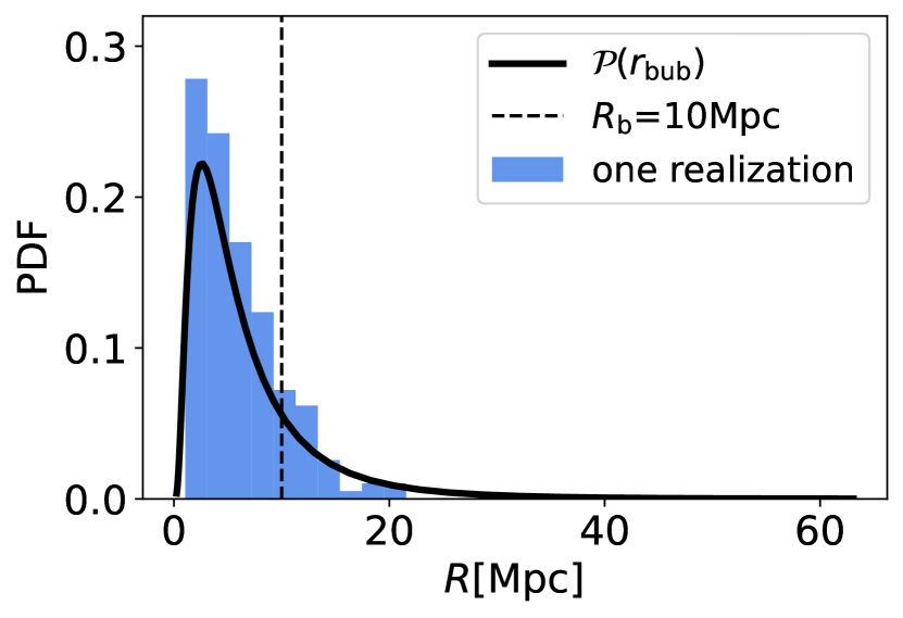
For simplicity, in this proof-of-concept work we ignore the dependence of the bubble size distribution in eq. (8), taking constant values of and . These choices in our algorithm roughly reproduce the ionized bubble scales seen in simulations during the early stages of the EoR (e.g., Mesinger & Furlanetto 2007; Giri et al. 2018; Lu et al. 2024b; Doussot & Semelin 2022; Neyer et al. 2024). Note that the from Eq. 8 does not directly translate to any of the metrics commonly used to characterize EoR morphology (e.g. Lin et al., 2016; Giri et al., 2018) and so comparisons must be done a-posteriori. In future work, we will calibrate Eq. (8) to EoR simulations, conditioning also on the matter field to account for the (modest) bias of HII regions at early times (e.g. Fig. 12 in Sobacchi & Mesinger, 2014). We show our assumed bubble size distribution in Fig. 4, as well as one realization in a cMpc3 volume.
For a given realization of EoR morphology and galaxy field (c.f. Fig. 1), we compute the damping wing optical depth by casting rays from the galaxy locations and summing the optical depth contributions from all HI patches along the LOS (e.g. Miralda-Escudé 1998):
| (9) |
where , is the wavelength at which we evaluate the optical depth, is the Lyman-alpha resonant wavelength and is the redshift of the emitting galaxy. is the Gunn-Peterson optical depth, , is the decay constant and Hz is the Lyman- resonant frequency. In the above equation, is given by:
| (10) |
The summation accounts for every neutral patch encountered along the LOS, with a given patch, , extending from to . We assume that ionized patches have no neutral hydrogen atoms so they do not contribute to the attenuation.
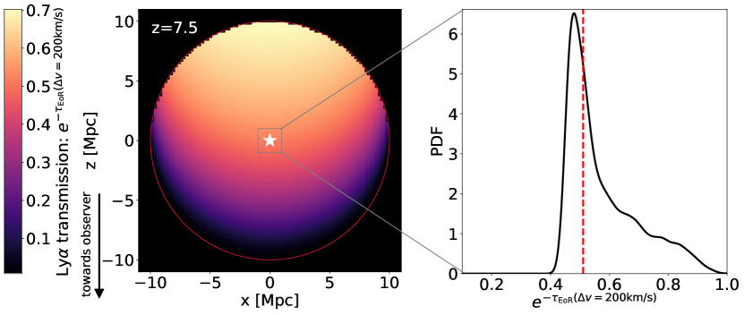
In the left panel of Fig 5 we show the mean IGM transmission, evaluated at km/s redward of the systemic redshift, as a function of position inside the central HII bubble of cMpc. The observer is located towards the bottom of the figure. This mean transmission was computed by averaging over 10000 realizations of EoR morphologies outside the central bubble, assuming (e.g. one such realization is shown in Fig. 1). As expected, there is a clear trend of increased transmission for galaxies located at the far end of the central HII bubble. The mean transmission is a function of the distance of the galaxy to the bubble edge in the direction towards the observer. In Lu et al. 2024b we used these trends to define empirical ”edge detection” algorithms.
However, at every location in the bubble, there is sizable sightline-to-sightline scatter in the IGM transmission. We quantify this in the right panel of Fig. 5, showing the transmission PDF constructed from the 10000 realizations of EoR morphology external to the central bubble. The sightlines used to compute this PDF originated from the location marked by the white star in the left panel. The PDF is quite broad and asymmetric (see also Fig. 2 in Mesinger & Furlanetto 2008b as well as Lu et al. 2024a). While it is difficult for the IGM to completely attenuate Ly for a galaxy located at the center of this bubble, some morphologies can result in large stretches of ionized IGM in the direction of the observer, driving a high-transmision tail in the PDF. The width of this PDF highlights the importance of accounting for stochasticity in the EoR morphology when interpreting galaxy Lyman alpha observations (e.g. Mesinger & Furlanetto 2008a; Mesinger et al. 2015; Mason et al. 2018; Bruton et al. 2023; Keating et al. 2024; Lu et al. 2024b).
2.4 Including NIRSpec noise
We take NIRSpec on JWST for our fiducial spectrograph in this work, which is already measuring Ly spectra from galaxy groups during the EoR (e.g. Tang et al. 2024a; Witstok et al. 2024a). To forward-model NIRSpec observations, we bin the observed flux to (high-resolution of NIRSpec), then add Gaussian noise to each spectral bin, with a standard deviation of ergs-1cm. This level of noise is obtainable with roughly a few hours of integration on NIRSpec (Bunker et al., 2023; Saxena et al., 2023; Tang et al., 2024a), and corresponds to an uncertainty on the integrated flux of ergs-1cm-2 (estimated assuming the emission line is spectrally unresolved). This can be further translated to limiting equivalent widths of () for (). We also find worse recovery assuming shallower observations, while our results do not improve significantly assuming deeper integrations than this fiducial value.
We re-bin the spectra to lower values of and test the inference with a coarser resolution. By performing additional binning, we lose some information on the observed line profile (e.g. Byrohl & Gronke, 2020), but lower the dimensionality of our likelihood (see Section 3). In future work, we will explore more sophisticated inference approaches that can scale to high-dimensional likelihoods (Cranmer et al., 2020; Anau Montel et al., 2024). Here we empirically settle on rest-frame as our bin width (i.e. ), corresponding to the medium resolution NIRSpec grating (Jakobsen et al., 2022, see Section 3).
3 Inferring the local HII bubble
With the above framework, we can create mock observations and corresponding forward models by sampling each of the terms in Eq. 2. We detail this procedure below.
3.1 Mock observations
We first construct a mock observation of galaxies in a survey volume of 20x20x20 cMpc3 (’’) at . This FoV is roughly motivated by JWST (corresponding to roughly 4 NIRSpec pointings), though in practice the forward-modeled volume should be tailored to the specific observation that is being interpreted. We place a bubble with radius 10 cMpc at the (arbitrarily-chosen) center of the volume, and construct the surrounding EoR morphology out to distances of 200 cMpc222Neutral IGM at larger distances contributes a negligible amount to the total attenuation, due to the steepness of the damping wing profile (Mesinger & Furlanetto, 2008a)., using the prescription from Sect. 2.3 and assuming . Below we demonstrate that our results are insensitive to these fiducial choices.
We assign random locations to the galaxies, with , using rejection sampling to ensure that on average 75% of the galaxies are inside HII regions (roughly matching results from simulations; e.g. Lu et al. 2024a). This is a very approximate way of accounting for galaxy bias, as both galaxies and HII regions are correlated to the large-scale matter field.333This is a reasonable approximation, as evidenced by our results in Section 5.2, where we apply our framework to simulations that self-consistently account for galaxy and HII region bias. Indeed, observations of galaxies demonstrate that the bias dominates clustering at larger scales ( tens of cMpc), while the smaller scales relevant for this work are dominated by Poisson noise (Bhowmick et al., 2018; Kragh Jespersen et al., 2024, Davies et al. in prep).
We generate UV magnitudes for each galaxy by sampling the UV luminosity function (LF) from Park et al. (2019) down to a magnitude limit of . Each galaxy is then assigned an emergent emission profile according to the procedure in the previous section, which is attenuated by its sightline through the realization of the EoR morphology. Finally, a noise realization is added to the binned flux to create a mock spectrum for each galaxy (c.f. Eq. 2).
3.2 Maximum likelihood estimate of bubble size and location
We then interpret this mock observation by forward modeling the observed flux for each galaxy, varying: (i) the position and radius of the central HII bubble; (ii) the surrounding EoR morphology; (iii) the neutral fraction of the Universe (within of the ”truth”, conservatively wider than current limits Qin et al. 2024); (iv) the emergent Lyman alpha flux given the galaxy’s observed (i.e. and ); (v) NIRSpec noise realizations.
For each forward model, we compute the likelihood of the mock observation, given the location and radius of the central HII region. Our sampling procedure effectively marginalizes over the unknowns (ii) – (v) from above. Because mapping out the joint likelihood over all of the observed galaxies would be numerically challenging, we make the simplifying assumption that the likelihood of the observed flux from each galaxy, , is independent from the other galaxies. This allows us to write the total likelihood of the observation as a product of the likelihoods of the individual galaxies:
| (11) |
While this assumption is clearly incorrect, here we present results only in terms of the maximum likelihood, . We demonstrate below that Eq. (11) provides an unbiased estimate of .444Ideally, we would want to map out the full posterior: where is a prior for the center location and radius of the HII bubble. However, including the correlations of the (non-Gaussian) likelihoods at the location of every galaxy is analytically not tractable, and would require high dimensional simulation based inference (e.g., de Santi et al., 2023; Lemos et al., 2023). We save this for future work.
It is important to note that we do not assume a Gaussian likelihood for the observed flux at each wavelength, as is commonly done. With high S/N spectra, correlations between flux bins can be significant. Instead we directly map out the joint PDF of flux over all wavelength bins, , using kernel density estimation over the forward-modeled spectra (see Appendix A for details). This preserves the covariances between the wavelength bins, and is commonly known as implicit likelihood or simulation based inference.
We demonstrate this procedure for the three galaxies shown in Fig. 1. The observed flux from galaxies ’A’, ’B’, and ’C’, is denoted in gray in the three panels of Fig. 6, left to right respectively. In blue we show the 68% C.L. of the likelihood assuming the correct HII bubble location and radius, . In red we show the 68% C.L. of the flux likelihood assuming the correct HII bubble location but a slightly smaller radius, . Galaxy ’A’ in this mock observation is outside of the central HII bubble, and therefore the true and slightly smaller values of result in the same likelihood. Galaxy ’B’ is located close to the center of the bubble, so both and give similar values of transmission (see Fig. 5). This results in only a slight preference for . On the other hand, galaxy ’C’ is located close to the edge of the bubble in Fig. 1. For that galaxy, we see that the observed spectrum in gray is more consistent with the correct likelihood in blue than with the incorrect one in red. Having a smaller bubble would imply more IGM attenuation on average at the location of this galaxy, making the observed strong Ly emission less likely. In this specific realization, the joint likelihood (Eq. 11) of the observed fluxes of ’A’, ’B’, and ’C’ is two times larger for the correct value of bubble radius than for the incorrect one. As one includes more and more galaxies, the maximum likelihood becomes increasingly peaked around the true values for the bubble size and location.
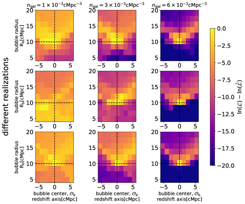
We illustrate this explicitly in Figure 7, in which we plot 2D slices through the log likelihood. The log likelihood normalized to the maximum value is indicated with the color bar. The vertical and horizontal axis in each panel correspond to the sampled bubble radius, , and redshift axis of the center, . The true values, = (10 cMpc, 0 cMpc), are demarcated with the dashed lines. The columns correspond to increasing number density of observed galaxies (left to right), while rows correspond to different realizations of forward models.
There are several interesting trends evident in Figure 7. Firstly, we see that increasing the number of observed galaxies (going from left to right in each row) results in an increasingly peaked likelihood, with the maximum settling on the true values for the bubble radius and location. Different realizations of the EoR morphology give different likelihood distributions when a small number of galaxies is observed. However, as the number density of observed galaxies is increased, the likelihood distributions between different realizations converge (i.e. all sources of stochasticity are ”averaged out”).
We also see a degeneracy between the redshift of the bubble center and its radius. Because the transmission is mostly determined by the distance to the bubble edge along the line of sight, moving the bubble center further away from the observer at a fixed radius is roughly degenerate with decreasing the radius at a fixed center location. This degeneracy is mitigated by having a larger number of sightlines to observed galaxies, allowing us to constrain the radius of curvature of the bubble.
4 How many galaxies do we need to confidently infer the local HII bubble?
In the previous section, we demonstrated that our framework gives an unbiased estimate of the HII region size and location when applied to a large galaxy sample. Here we quantify just how ”large” does this galaxy sample need to be, in order for us to be confident in our results. For this purpose we define two figures of merit:
| (12) | ||||
| (14) |
Here, and are the maximum likelihood estimates of the HII bubble center and radius computed from a galaxy field with number density , and Errloc and Errrad are the corresponding fractional errors (normalized to the true bubble radius).
Since we are calculating the likelihood on the grid, we can say that our framework ”has found” the optimal bubble when the fiducial and inferred locations and radii coincide, i.e. Err Err. In that case, the error of location and radius is below the grid on which we calculate the likelihood (cMpc in our fiducial case, corresponding to a % fractional error).
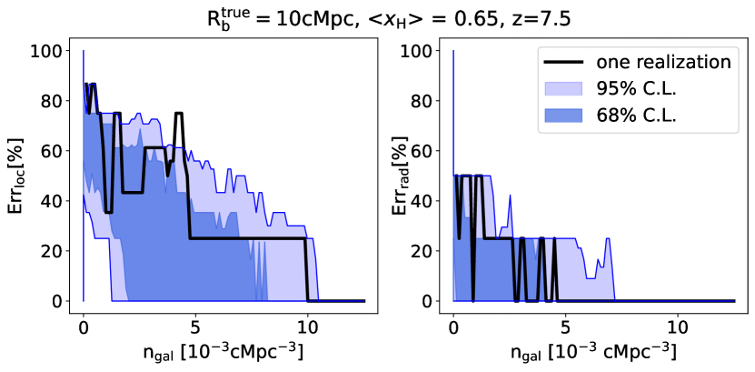
The solid black curve in Fig. 8 shows how these fractional errors change with galaxy number density for a single realization. Here the realization of EoR morphology and ”observed” galaxies are held constant, with the maximum likelihood computed each time a new ”observed” galaxy is added. The more galaxies we observe, the smaller the error on our inferred HII bubble location and radius. The sizable stochasticity in galaxy properties and sightline-to-sightline scatter in the IGM opacity manifest as ”noise” in this evolution, making it non-monotonic. Nevertheless, even a single galaxy is able to shrink the fractional error by a factor of two from our prior range, ruling out extreme values.
We repeat this calculation with 100 different realizations of the mock observation (EoR morphology and observed galaxy samples). In Fig. 8 we show the resulting 68% and 95% C.L. on the fractional errors as more and more galaxies are added to the field. We see that in 68% (95%) of cases, number densities of () cMpc-3 are sufficient to obtain a error on the center position. The corresponding requirements are () cMpc-3 for error on the bubble radius (comparable to Lu et al. 2024b). In other words, Ly spectra from galaxies per cMpc3 are required to be 95% confident that the HII bubble location and size recovered by our method is accurate at 1 cMpc. This corresponds roughly to 80 galaxies in 2x2 tiled pointings with JWST/NIRSpec.
4.1 Including a prior on the emergent Lyman alpha
In this work we assume the emergent Lyman alpha emission follows post-EoR empirical relations, as described in Section 2.1. Beyond this, we assume no prior knowledge on each galaxy’s intrinsic emission. However, lower opacity nebular lines such as the Balmer lines (H, H), can provide complimentary estimates of the intrinsic production of Lyman alpha photons (e.g. Hayes et al. 2023; Saxena et al. 2023; Chen et al. 2024). In this section we repeat the analysis from above, but including a simple prior on the emergent Ly emission.
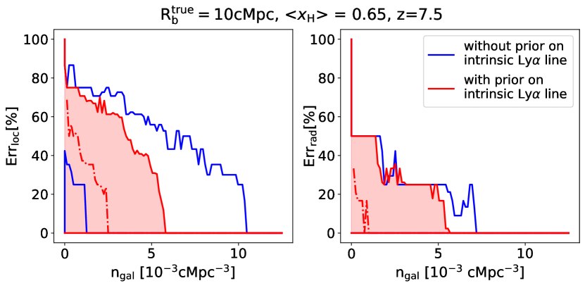
Specifically, we apply rejection sampling to keep only those forward-models for which the transmission is within of the true one (or putting an upper bound if )555A detection of Balmer lines puts constraints on the production rate of Lyman alpha photons, who then have to pass through the ISM, CGM and IGM. Our distribution of Lyman- equivalent widths and profile shapes described in Section. 2.2 effectively already includes radiative transfer and escape through the ISM + CGM, which we assume does not evolve significantly with redshift at . Thus our prior is effectively a prior on the IGM transmission. We leave a self-consistent treatment of the redshift evolution of ISM+CGM escape fraction and IGM transmission for future work. Then we calculate the likelihood the same way as we did in Section 3. The width of the prior is motivated by current observations using JWST (c.f. Saxena et al. 2023 for H, and Lin et al. 2024 for H from ground instruments). Note that H observations above are not possible with NIRSpec. For higher redshifts, we therefore have to rely on a fainter H. Despite this, H is regularly observed in high galaxies, so using the prior for all galaxies is not unreasonable (e.g., Meyer et al., 2024).
In Fig. 9 we show the 95% C.L. on the fractional errors with (red) and without (blue; same as Fig. 8) the prior information on the emergent Lyman alpha emission. We see that using additional nebular lines to constrain the emergent Lyman alpha emission can reduce by a factor of two the required number of galaxies to obtain the same constraints.
4.2 Results for different bubble sizes
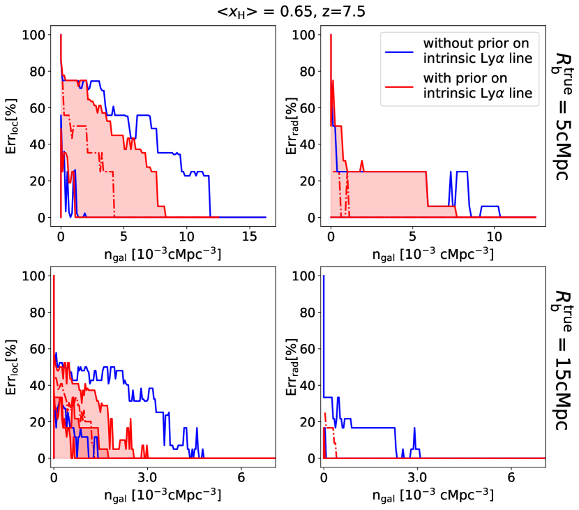
Our fiducial choice for the radius of the central HII bubble is Mpc, motivated by HII bubble sizes in the early stages of the EoR. Here we test the performance of our pipeline for other radii, and Mpc.
In the top (bottom) panels of Fig. 10 we show the analysis with and without the 20% prior on the emergent emission, assuming Mpc (Mpc). Comparing to the fiducial results in Fig. 9, we see that fewer galaxies are required to infer the size and location for larger HII bubbles. For cMpc roughly 2-3 times fewer galaxies are required to constrain the HII bubble with the same accuracy, compared to cMpc. This is most likely due to the fact that the larger bubbles allow for a broader range of IGM opacities. Galaxies inside small bubbles have roughly the same attenuation regardless of their relative location inside the bubble. In contrast, for larger bubbles there is a noticeable difference between the (average) attenuation on the near side and far of the bubble, allowing us to more easily constrain their geometry (c.f. the left panel of Fig. 5).
5 Building confidence in our framework
In this section, we explore how do our results depend on our model assumptions. To do this, we apply our framework on a different reionization morphology and on different emergent EW distributions. Even though our framework is a proof-of-concept, having it perform well on such ”out-of-distribution” tests would help build confidence that it is not sensitive to uncertainties in the details of our model.
5.1 Different EW distribution
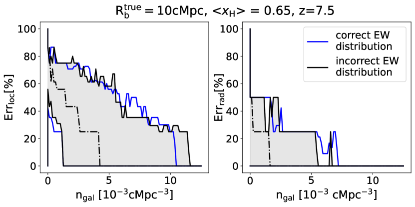
First, we test the performance of our pipeline assuming the emergent Lyman- luminosities follow a different EW distribution than the we use in our forward-models (Sec. 2.2). Specifically, we generate mock observations assuming a Gaussian distribution from Treu et al. (2012) (based on Stark et al. (2011), but with the same parameters as in Section 2.2):
| (15) | ||||
We then interpret these mock observations with our fiducial pipeline, which uses the exponential EW distribution from Eq. 7.
The resulting 95% C.L. on the fractional errors are highlighted in gray in Fig. 11. In blue, we show the same 95% C.L. from Fig. 8, which use same EW distribution for the forward models and the mock observation. The fact that the gray and blue regions demarcate roughly the same fractional errors suggests that our analysis is not sensitive to the choice of EW distribution.
5.2 Demonstration on a 3D reionization simulation
Because this work is intended as a proof-of-concept, throughout we made several simplifying assumptions. For example, our reionization morphology is generated by overlapping ionized spheres and we have only a simplified treatment for galaxy – HII bubble bias. Including a more realistic bias for both galaxies and HII regions would be straightforward to do analytically, but it is necessary? Here we test how our simple model performs on self-consistent 3D simulations of reionization.
We apply our framework on the galaxy catalogs and ionization maps from the simulations of Lu et al. (2024b), generated with the public 21cmFAST code (Mesinger & Furlanetto, 2007; Mesinger et al., 2011; Murray et al., 2020). These simulations capture the complex morphology of reionization, which is self-consistently generated from the underlying galaxy fields. We process the galaxies with the procedure outlined in Section 2 to create mocks on which we can perform the inference.
We use two ionization boxes, one at and . We select ionized bubbles and associated galaxies that match the volumes we use in our fiducial set-up, specifically 20x20x20 cMpc. When applying the inference framework to real data, one should of course tailor the forward models to match the specific details of the survey.
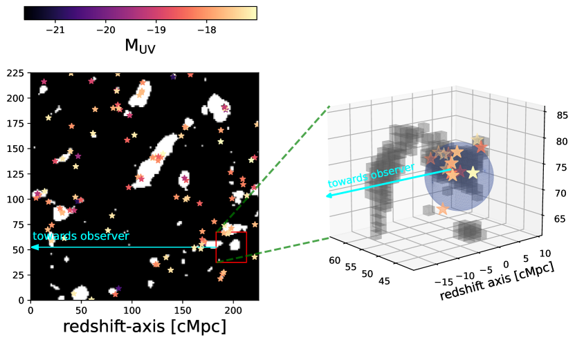
We illustrate the results in Figures 12 and 13, for a couple of example surveys at and , respectively. In the left panels, we show 1.5 cMpc thick slices through the simulation boxes. Ionized/neutral regions are shown as white/black. The brightest galaxies are shown with stars, whose colors correspond to their UV magnitudes. The line of sight direction used to compute the IGM opacity for each observed galaxy is indicated with the arrow.
The volumes of the mock surveys are illustrated with the zoom-ins on the right. Here, gray cells show the ionized voxels of the simulation, and the blue sphere is the maximum likelihood solution for the central HII region. We assumed all galaxies inside this 20x20x20 cMpc volume brighter than are observed with NIRSpec. This corresponds to galaxies at ().
We see from the zoom-ins in these figures that the inferred HII regions in blue provide a reasonable characterization of the ”true” HII region in gray. This gives us confidence in our simplified treatment of the EoR morphology and the associated spatial correlation with galaxies. As mentioned above, we will tailor future applications to actual NIRSpec surveys of galaxy groups.
6 JWST observational requirements
We currently have several spectroscopically-targeted fields containing groups of galaxies with detection in Lyman-, such as COSMOS (Endsley & Stark, 2022; Witten et al., 2024), EGS (Oesch et al., 2015; Zitrin et al., 2015; Roberts-Borsani et al., 2016; Tilvi et al., 2020; Leonova et al., 2022; Larson et al., 2022; Jung et al., 2022; Tang et al., 2023, 2024b; Chen et al., 2024; Napolitano et al., 2024), BDF (Castellano et al., 2016, 2018), GOODS-N (Oesch et al., 2016; Eisenstein et al., 2023; Bunker et al., 2023; Tacchella et al., 2023) and GOODS-S (Witstok et al., 2024b; Tang et al., 2024b). Although the number densities are a factor of few lower (cMpc-3) than the required values in Section. 4, the data sets are expanding rapidly. On-going and proposed programs are extending fields and going deeper, resulting in larger areas and number densities. Here we quantify in more detail the JWST survey requirements in order to be able to robustly constrain HII bubbles with our procedure.
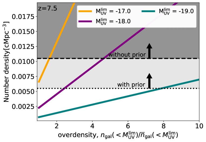
In Fig. 14 we show the number density of galaxies as a function of limiting UV magnitude, and galaxy overdensity, .We plot three curves corresponding to = -17, -18, -19. We demarcate in gray the required number density for accurate HII bubble recovery we found in the previous section; the lower/upper range correspond to including/not including a prior on the emergent Ly emission from Balmer lines (c.f. Section 4).
At the mean number density, we would require the photometric survey to detect galaxies down to -17.0 – -17.5. The quoted range spans what can be achieved with or without a prior on the Lyman alpha production rate from Balmer lines. In an unlensed field, obtaining such number densities would require roughly hours of integration with NIRCam on JWST (estimated based on exposure times in Morishita et al., 2024, for 4 pointings): achievable, but ambitions.
However, several current fields are known to contain overdensities. For example, COSMOS contains a 140 pMpc3 volume that is estimated to be three times overdense at (Endsley & Stark, 2022), while EGS is estimated to contain a pMpc3 volume that is also overdense at (Zitrin et al., 2015; Leonova et al., 2022; Larson et al., 2022; Tang et al., 2023; Chen et al., 2024; Lu et al., 2024a). Also, GOODS-S and GOODS-N contain 4x and 8x overdensities over volumes larger than the fiducial one used in this work (62 arcmin2x Tang et al., 2024b). Furthermore, one of the most distant observed LAE is also believed to be located in an overdensity (up to overdense at in pMpc3 volume; Oesch et al., 2016; Bunker et al., 2023; Tacchella et al., 2023, see also Lu et al. 2024a for other examples). Observing a field with an overdensity of three (eight) would require photometric completeness down to -18.5 – -18 (-19 – -18.5). This would require ”only” 50 (4.2) hours of integration with NIRCam.
These candidates then require spectroscopic follow-up. For spectroscopic confirmation, the best candidate is [OIII]5007 emission line. The [OIII] emission line is routinely observed with JWST (e.g., Endsley et al., 2023, 2024; Meyer et al., 2024). We can estimate the required exposure time for detecting [OIII] line by assuming the dependent distribution of equivalent widths from Endsley et al. (2024). For that distribution, the equivalent width limit for detecting galaxies at is . Obtaining such an equivalent width (at ) at with the G395M filter requires hours per pointing. The number density requirement (and thus exposure time) would increase if we do not detect H as required to put a prior on the intrinsic Lyman- emission. It would also increase if the [OIII] distribution is lower at lower magnitudes.
Following that, to detect Lyman at a noise level of erg s-1cm-2 (corresponding to a detection of a line of W) would require hours with G140M per pointing. These numbers are comparable to existing large JWST surveys (Eisenstein et al., 2023).
We also note that the volume of the potential JWST surveys used for this analysis has a direct impact on the sizes of the HII regions that can be inferred (see also Lu et al. 2024b). Tiled surveys of the same depth but larger volumes, could hope to detect correspondingly-larger HII regions. The fact that larger HII regions occur later in the EoR, with a correspondingly higher galaxy number densities, might mitigate the integration time required. We postpone more systematic survey design to subsequent work in which we apply our framework to simulated 3D EoR lightcones.
Another interesting approach could be coupling the framework from Lu et al. (2024b) with the one outlined in this work. The large-scale empirical method from Lu et al. (2024b) could isolate ”interesting” sub-volumes that could then be analyzed with the quantitative inference approach presented here.
7 Conclusions
The morphology of reionization tells us which galaxies dominated the epoch of cosmic reionization. Individual bubbles surrounding groups of galaxies encode information on the contribution of unseen, faint sources and allow us to correlate the properties of bubbles and the galaxies they host.
In this work we build a framework to use Lyman- observations from JWST NIRspec to constrain ionization morphology around a group of galaxies. Our framework for the first time uses complementary information from sightlines to neighboring galaxies, and samples all important sources of stochasticity to robustly place constraints on the size and position of local HII bubbles.
We find that Ly spectra from galaxies per cMpc3 are required to be 95% confident that the HII bubble location and size recovered by our method is accurate to better than 1.5 cMpc. This corresponds roughly to 80 galaxies in 2x2 tiled pointings with JWST/NIRSpec. These requirements can be reduced by using additional nebular lines (for example H) to constrain the intrinsic Lyman alpha emission. We find that a simple prior on the emergent Lyman- emission reduces by a factor of two the required number of galaxies to obtain the same constraints. Such number densities are achievable with a targeted survey with completeness down to – -19, depending on the over-density of the field.
We demonstrate that our framework is not sensitive to the assumed distribution for the emergent Lyman alpha emission. We also find accurate recovery of ionized bubbles when applied to 3D EoR simulations.
Our pipeline can be applied to existing observations of Lyman- spectra from galaxy groups. Additionally, observational requirements for a statistical detection of local HII regions presented here can be used to design complimentary, new JWST surveys. Applying our framework to multiple, independent fields would allow us to constrain the distribution of bubble sizes, which helps us understand which galaxies reionized the Universe.
8 Data availability
The code related to the work is publicly available at \faGithubIvanNikolic21/Lyman alpha bubbles.
Acknowledgements.
We gratefully acknowledge computational resources of the Center for High Performance Computing (CHPC) at SNS. AM acknowledges support from the Italian Ministry of Universities and Research (MUR) through the PRIN project ”Optimal inference from radio images of the epoch of reionization”, the PNRR project ”Centro Nazionale di Ricerca in High Performance Computing, Big Data e Quantum Computing”. CAM and TYL acknowledge support by the VILLUM FONDEN under grant 37459. CAM acknowledges support from the Carlsberg Foundation under grant CF22-1322.References
- Almada Monter & Gronke (2024) Almada Monter, S. & Gronke, M. 2024, MNRAS, 534, L7
- Anau Montel et al. (2024) Anau Montel, N., Alvey, J., & Weniger, C. 2024, MNRAS, 530, 4107
- Bhowmick et al. (2018) Bhowmick, A. K., Campbell, D., Di Matteo, T., & Feng, Y. 2018, MNRAS, 480, 3177
- Bolan et al. (2024) Bolan, P., Bradăc, M., Lemaux, B. C., et al. 2024, MNRAS, 531, 2998
- Bolan et al. (2022) Bolan, P., Lemaux, B. C., Mason, C., et al. 2022, MNRAS, 517, 3263
- Bosman et al. (2022) Bosman, S. E. I., Davies, F. B., Becker, G. D., et al. 2022, MNRAS, 514, 55
- Bruton et al. (2023) Bruton, S., Scarlata, C., Haardt, F., et al. 2023, ApJ, 953, 29
- Bunker et al. (2023) Bunker, A. J., Saxena, A., Cameron, A. J., et al. 2023, A&A, 677, A88
- Byrohl & Gronke (2020) Byrohl, C. & Gronke, M. 2020, A&A, 642, L16
- Castellano et al. (2016) Castellano, M., Dayal, P., Pentericci, L., et al. 2016, ApJ, 818, L3
- Castellano et al. (2018) Castellano, M., Pentericci, L., Vanzella, E., et al. 2018, ApJ, 863, L3
- Chen et al. (2024) Chen, Z., Stark, D. P., Mason, C., et al. 2024, MNRAS, 528, 7052
- Cranmer et al. (2020) Cranmer, K., Brehmer, J., & Louppe, G. 2020, Proceedings of the National Academy of Science, 117, 30055
- De Barros et al. (2017) De Barros, S., Pentericci, L., Vanzella, E., et al. 2017, A&A, 608, A123
- de Santi et al. (2023) de Santi, N. S. M., Villaescusa-Navarro, F., Abramo, L. R., et al. 2023, arXiv e-prints, arXiv:2310.15234
- Dijkstra (2014) Dijkstra, M. 2014, PASA, 31, e040
- Dijkstra et al. (2011) Dijkstra, M., Mesinger, A., & Wyithe, J. S. B. 2011, MNRAS, 414, 2139
- Dijkstra & Wyithe (2012) Dijkstra, M. & Wyithe, J. S. B. 2012, MNRAS, 419, 3181
- Doussot & Semelin (2022) Doussot, A. & Semelin, B. 2022, A&A, 667, A118
- Eisenstein et al. (2023) Eisenstein, D. J., Willott, C., Alberts, S., et al. 2023, arXiv e-prints, arXiv:2306.02465
- Endsley & Stark (2022) Endsley, R. & Stark, D. P. 2022, MNRAS, 511, 6042
- Endsley et al. (2023) Endsley, R., Stark, D. P., Whitler, L., et al. 2023, MNRAS, 524, 2312
- Endsley et al. (2024) Endsley, R., Stark, D. P., Whitler, L., et al. 2024, MNRAS, 533, 1111
- Ghara et al. (2018) Ghara, R., Mellema, G., Giri, S. K., et al. 2018, MNRAS, 476, 1741
- Giri et al. (2018) Giri, S. K., Mellema, G., Dixon, K. L., & Iliev, I. T. 2018, MNRAS, 473, 2949
- Hayes et al. (2023) Hayes, M. J., Runnholm, A., Scarlata, C., Gronke, M., & Rivera-Thorsen, T. E. 2023, MNRAS, 520, 5903
- Hayes & Scarlata (2023) Hayes, M. J. & Scarlata, C. 2023, ApJ, 954, L14
- Hu et al. (2023) Hu, W., Martin, C. L., Gronke, M., et al. 2023, ApJ, 956, 39
- Hutter et al. (2023) Hutter, A., Trebitsch, M., Dayal, P., et al. 2023, MNRAS, 524, 6124
- Jakobsen et al. (2022) Jakobsen, P., Ferruit, P., Alves de Oliveira, C., et al. 2022, A&A, 661, A80
- Jones et al. (2024) Jones, G. C., Bunker, A. J., Saxena, A., et al. 2024, A&A, 683, A238
- Jung et al. (2020) Jung, I., Finkelstein, S. L., Dickinson, M., et al. 2020, ApJ, 904, 144
- Jung et al. (2022) Jung, I., Finkelstein, S. L., Larson, R. L., et al. 2022, arXiv e-prints, arXiv:2212.09850
- Keating et al. (2024) Keating, L. C., Puchwein, E., Bolton, J. S., Haehnelt, M. G., & Kulkarni, G. 2024, MNRAS, 531, L34
- Kragh Jespersen et al. (2024) Kragh Jespersen, C., Steinhardt, C. L., Somerville, R. S., & Lovell, C. C. 2024, arXiv e-prints, arXiv:2403.00050
- Larson et al. (2022) Larson, R. L., Finkelstein, S. L., Hutchison, T. A., et al. 2022, ApJ, 930, 104
- Laursen et al. (2011) Laursen, P., Sommer-Larsen, J., & Razoumov, A. O. 2011, ApJ, 728, 52
- Lemos et al. (2023) Lemos, P., Parker, L. H., Hahn, C., et al. 2023, in Machine Learning for Astrophysics, 18
- Leonova et al. (2022) Leonova, E., Oesch, P. A., Qin, Y., et al. 2022, MNRAS, 515, 5790
- Lin et al. (2024) Lin, X., Cai, Z., Wu, Y., et al. 2024, ApJS, 272, 33
- Lin et al. (2016) Lin, Y., Oh, S. P., Furlanetto, S. R., & Sutter, P. M. 2016, MNRAS, 461, 3361
- Lu et al. (2024a) Lu, T.-Y., Mason, C. A., Hutter, A., et al. 2024a, MNRAS, 528, 4872
- Lu et al. (2024b) Lu, T.-Y., Mason, C. A., Mesinger, A., et al. 2024b, arXiv e-prints, arXiv:2411.04176
- Mason et al. (2018) Mason, C. A., Treu, T., Dijkstra, M., et al. 2018, ApJ, 856, 2
- McQuinn et al. (2007) McQuinn, M., Lidz, A., Zahn, O., et al. 2007, MNRAS, 377, 1043
- Mesinger et al. (2015) Mesinger, A., Aykutalp, A., Vanzella, E., et al. 2015, MNRAS, 446, 566
- Mesinger & Furlanetto (2007) Mesinger, A. & Furlanetto, S. 2007, ApJ, 669, 663
- Mesinger et al. (2011) Mesinger, A., Furlanetto, S., & Cen, R. 2011, MNRAS, 411, 955
- Mesinger & Furlanetto (2008a) Mesinger, A. & Furlanetto, S. R. 2008a, MNRAS, 385, 1348
- Mesinger & Furlanetto (2008b) Mesinger, A. & Furlanetto, S. R. 2008b, MNRAS, 386, 1990
- Mesinger et al. (2016) Mesinger, A., Greig, B., & Sobacchi, E. 2016, MNRAS, 459, 2342
- Meyer et al. (2024) Meyer, R., Oesch, P., Giovinazzo, E., et al. 2024, arXiv preprint arXiv:2405.05111
- Meyer et al. (2021) Meyer, R. A., Laporte, N., Ellis, R. S., Verhamme, A., & Garel, T. 2021, MNRAS, 500, 558
- Miralda-Escudé (1998) Miralda-Escudé, J. 1998, ApJ, 501, 15
- Morishita et al. (2024) Morishita, T., Mason, C. A., Kreilgaard, K. C., et al. 2024, arXiv e-prints, arXiv:2412.04211
- Murray et al. (2020) Murray, S., Greig, B., Mesinger, A., et al. 2020, The Journal of Open Source Software, 5, 2582
- Nakane et al. (2024) Nakane, M., Ouchi, M., Nakajima, K., et al. 2024, ApJ, 967, 28
- Napolitano et al. (2024) Napolitano, L., Pentericci, L., Santini, P., et al. 2024, A&A, 688, A106
- Neufeld (1990) Neufeld, D. A. 1990, ApJ, 350, 216
- Neyer et al. (2024) Neyer, M., Smith, A., Kannan, R., et al. 2024, MNRAS, 531, 2943
- Oesch et al. (2016) Oesch, P. A., Brammer, G., van Dokkum, P. G., et al. 2016, ApJ, 819, 129
- Oesch et al. (2015) Oesch, P. A., van Dokkum, P. G., Illingworth, G. D., et al. 2015, ApJ, 804, L30
- Orlitová et al. (2018) Orlitová, I., Verhamme, A., Henry, A., et al. 2018, A&A, 616, A60
- Park et al. (2019) Park, J., Mesinger, A., Greig, B., & Gillet, N. 2019, MNRAS, 484, 933
- Planck Collaboration et al. (2020) Planck Collaboration, Aghanim, N., Akrami, Y., et al. 2020, A&A, 641, A6
- Qin et al. (2021) Qin, Y., Mesinger, A., Bosman, S. E. I., & Viel, M. 2021, MNRAS, 506, 2390
- Qin et al. (2024) Qin, Y., Mesinger, A., Prelogović, D., et al. 2024, arXiv e-prints, arXiv:2412.00799
- Roberts-Borsani et al. (2016) Roberts-Borsani, G. W., Bouwens, R. J., Oesch, P. A., et al. 2016, ApJ, 823, 143
- Saxena et al. (2023) Saxena, A., Robertson, B. E., Bunker, A. J., et al. 2023, A&A, 678, A68
- Sobacchi & Mesinger (2014) Sobacchi, E. & Mesinger, A. 2014, MNRAS, 440, 1662
- Stark et al. (2017) Stark, D. P., Ellis, R. S., Charlot, S., et al. 2017, MNRAS, 464, 469
- Stark et al. (2010) Stark, D. P., Ellis, R. S., Chiu, K., Ouchi, M., & Bunker, A. 2010, MNRAS, 408, 1628
- Stark et al. (2011) Stark, D. P., Ellis, R. S., & Ouchi, M. 2011, ApJ, 728, L2
- Steidel et al. (2014) Steidel, C. C., Rudie, G. C., Strom, A. L., et al. 2014, ApJ, 795, 165
- Tacchella et al. (2023) Tacchella, S., Eisenstein, D. J., Hainline, K., et al. 2023, ApJ, 952, 74
- Tang et al. (2023) Tang, M., Stark, D. P., Chen, Z., et al. 2023, MNRAS, 526, 1657
- Tang et al. (2024a) Tang, M., Stark, D. P., Ellis, R. S., et al. 2024a, MNRAS, 531, 2701
- Tang et al. (2024b) Tang, M., Stark, D. P., Topping, M. W., Mason, C., & Ellis, R. S. 2024b, arXiv e-prints, arXiv:2408.01507
- Tilvi et al. (2020) Tilvi, V., Malhotra, S., Rhoads, J. E., et al. 2020, ApJ, 891, L10
- Treu et al. (2012) Treu, T., Trenti, M., Stiavelli, M., Auger, M. W., & Bradley, L. D. 2012, ApJ, 747, 27
- Umeda et al. (2024) Umeda, H., Ouchi, M., Nakajima, K., et al. 2024, ApJ, 971, 124
- Verhamme et al. (2018) Verhamme, A., Garel, T., Ventou, E., et al. 2018, MNRAS, 478, L60
- Witstok et al. (2024a) Witstok, J., Maiolino, R., Smit, R., et al. 2024a, arXiv e-prints, arXiv:2404.05724
- Witstok et al. (2024b) Witstok, J., Smit, R., Saxena, A., et al. 2024b, A&A, 682, A40
- Witten et al. (2024) Witten, C., Laporte, N., Martin-Alvarez, S., et al. 2024, Nature Astronomy, 8, 384
- Yamada et al. (2012) Yamada, T., Matsuda, Y., Kousai, K., et al. 2012, ApJ, 751, 29
- Zahn et al. (2011) Zahn, O., Mesinger, A., McQuinn, M., et al. 2011, MNRAS, 414, 727
- Zitrin et al. (2015) Zitrin, A., Labbé, I., Belli, S., et al. 2015, ApJ, 810, L12
Appendix A Mapping the joint distribution over all flux bins with kernel density estimation
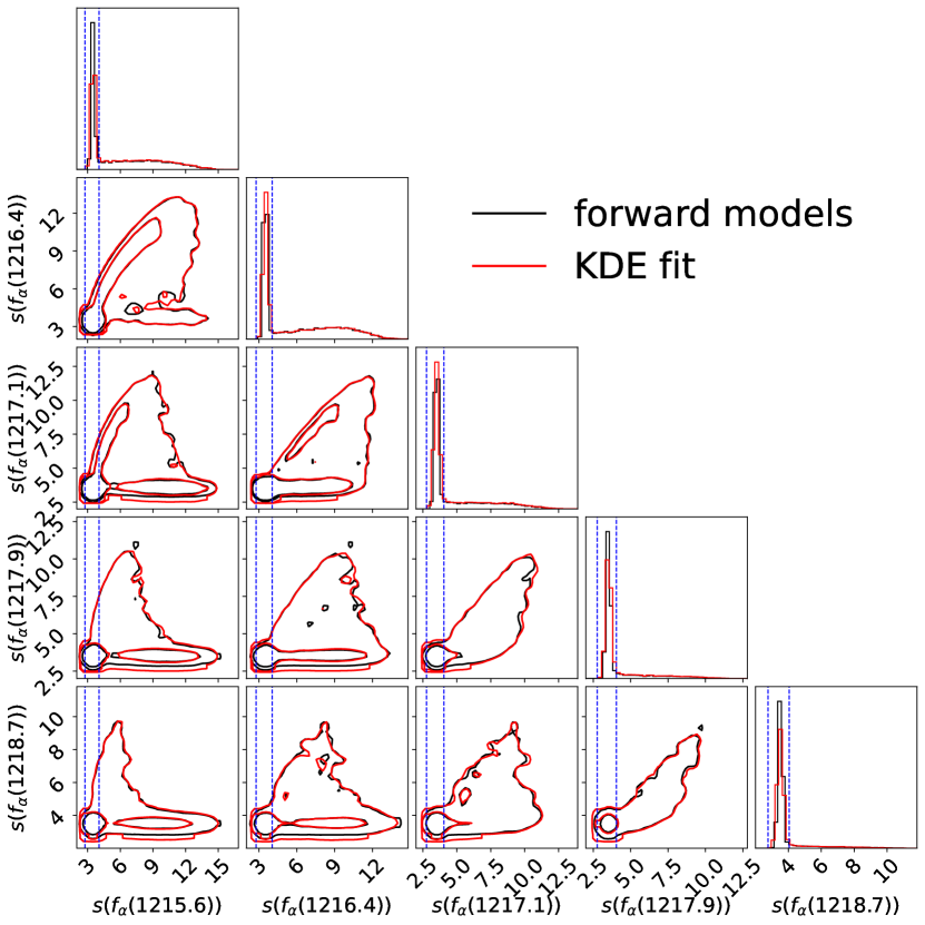
In Section 3 we showed how we generate forward models of JWST observations. Here we detail how we compute flux PDFs, i.e. likelihoods, in the space of local HII region parameters. In Fig. 15 in black we show a corner plot of forward models of a galaxy located in the center of its local HII region with size cMpc. Black contours display and C.L. of the distribution respectively. We only show bins in our fiducial resolution () where the Lyman- emission is located. In order to fit a density estimator to obtain a smooth PDF, we scale fluxes by a common function:
| (16) |
Each column and row represents one wavelength bin of the flux scaled by the function in Eq. 16. We fit a Kernel Density Estimator to the forward models displayed in the corner plot with an exponential kernel of bandwidth . The scaling function and bandwidth were selected by optimizing the results of Section 4 (i.e., kernel density bandwidth and normalizing function that allows the inference of bubble properties for the least number of galaxies). We show contours of the fitted KDE in red in Fig. 15.
Several features can be noted in Fig.15. Firstly, there is a strong peak for lower values of . This peak corresponds to the noise which is Gaussian by construction. This is further demonstrated with the blue dashed lines that show noise levels from Section. 2.4. On the other hand, there are additional features for larger values of . These features represent the Lyman- signal that is higher than the noise. It is important to note that there is non-negligible correlation between different bins and the distribution is highly non-trivial. This shows that a simple likelihood that uses independent Gaussians for each bin would potentially bias the inference and an approach that fits the whole distribution is necessary.
KDE fits the data for all of the bins, in the noise and signal regimes. There is a small overestimation of the width of the distribution for bins that are noise-dominated. Since these bins do not give a lot of information for Lyman- inference, our KDE is not biasing results.