Bayesian estimation of coupling strength and heterogeneity in a coupled oscillator model from macroscopic quantities
Abstract
Various macroscopic oscillations, such as the heartbeat and the flushing of fireflies, are created by synchronizing oscillatory units (oscillators). To elucidate the mechanism of synchronization, several coupled oscillator models have been devised and extensively analyzed. Although parameter estimation of these models has also been actively investigated, most of the proposed methods are based on the data from individual oscillators, not from macroscopic quantities. In the present study, we propose a Bayesian framework to estimate the model parameters of coupled oscillator models, using the time series data of the Kuramoto order parameter as the only given data. We adopt the exchange Monte Carlo method for the efficient estimation of the posterior distribution and marginal likelihood. Numerical experiments are performed to confirm the validity of our method and examine the dependence of the estimation error on the observational noise and system size.
I Introduction
Just as the collective motion of the heart originates from the cooperative individual cardiomyocytes, some oscillations in nature and society are created by multiple oscillatory units (oscillators) that are synchronizing [1]. Other examples of synchronization include the rhythmic flushing of firefly populations [2], pathologic synchronized brain activities in several neuronal disorders [3, 4, 5], and the spontaneous large vibration of the London’s Millenium Bridge created by coordinated pedestrians [6].
To elucidate the mechanism of synchronization, several types of coupled phase-oscillator models, such as the Kuramoto model [7], have been devised and extensively analyzed in a theoretical context [8, 9, 10]. There are also attempts to utilize coupled oscillator models for practical applications, e.g., for the further understanding of the mechanism of neuronal disorders [11] or the power grid [12, 13], and for the development of high-speed computers (coherent Ising machines) [14].
Among parameters in coupled oscillator models, two are particularly crucial for achieving synchrony: the strength of the interaction between the oscillators (coupling strength) and the variation among the oscillator population (heterogeneity). If the heterogeneity is sufficiently large compared to the coupling strength, synchronization is unlikely to occur, and vice versa. To understand and control real synchronization phenomena using coupled oscillator models, it is crucial to estimate these model parameters from observed data.
Although there are numerous previous studies on the data-driven estimation of coupled oscillator models [15, 16, 17, 18], most of these studies estimate from time series data of all individual oscillators. In practical data acquisition, the number of measurable oscillating units (e.g., cells) can be limited. Furthermore, the computational cost of estimation increases with the amount of data. Therefore, developing estimation methods that utilize macroscopic quantities reflecting collective oscillations, rather than relying on individual observations of each oscillator, is crucial.
One example of such macroscopic quantities is the Kuramoto order parameter, which is widely used as an index of synchronization [1, 9, 19]. Within a theoretical framework called the Ott-Antonsen ansatz [20, 21], the dynamics of the Kuramoto order parameter can be analytically derived for several coupled oscillator models in the thermodynamic limit. By using the analytical solution from Ott-Antonsen ansatz, we expect that efficient parameter estimation can be achieved. Although a recent study [22] employed the linear and nonlinear response theory for the parameter estimation from the time series of the generalized order parameter (Daido order parameter [23]), no previous studies, to the best of our knowledge, have attempted to estimate the parameters of coupled oscillator models by using the analytical results from the Ott-Antonsen ansatz.
Among various estimation methods, Bayesian inference has an advantage in providing the posterior distribution of parameters, from which we can determine the confidence interval of the estimated value. Bayesian inference also provides the marginal likelihood, which quantifies the probability of the estimation model for a given dataset and can be used for model comparison. We expect that adopting the Bayesian approach leads to an accurate and reliable estimation of models.
In the present study, we aim to use Bayesian inference to estimate the model parameters of the Kuramoto model, a type of coupled oscillator system, from the time series data of the Kuramoto order parameter. According to the Ott-Antonsen ansatz, the dynamics of the Kuramoto order parameter can be analytically obtained in a closed form with model parameters. We use this analytical expression as a forward model for the parameter estimation.
To enhance estimation accuracy and efficiency, we employ the exchange Monte Carlo (EMC) method for calculating posterior distribution and marginal likelihood. Originally introduced in the field of statistical physics [24], the EMC method has been extensively applied to a wide range of Bayesian inference problems [25, 26, 27, 28, 29]. In the context of coupled oscillator systems, although a previous study has used the EMC method for network optimization [30], its application to parameter estimation has not been investigated, as far as we know. We believe that our study is the first attempt in both applying the theoretical results from Ott-Antonsen ansatz and adopting the Bayesian approach with the EMC method to estimate the parameters of coupled oscillator models.
The remainder of this paper is organized as follows: in Sec. II, we describe the model and the estimation framework. We introduce the Kuramoto model and its analytical solution based on the Ott-Antonsen ansatz in Sec. II.1, and then we describe the EMC algorithm in Sec. II.2. The results of numerical experiments are summarized in Sec. III, in which we generate the artificial datasets and examine the dependence of the estimation accuracy on the observational noise and system size. We first use the same model for both data generation and estimation process to confirm the validity of our framework (Sec. III.2), and then we use the Kuramoto model (1) as the data generation model to investigate the finite size effect of the number of oscillators (Sec. III.3). Finally, we describe the discussion and conclusion in Sec. IV.
II Theory
II.1 Model
II.1.1 Kuramoto model and Kuramoto order parameter
We consider the following Kuramoto model:
| (1) |
for . Here, and denote the phase and the natural frequency of the -th oscillator, is the strength of the coupling among oscillators, and is the number of the oscillators. We assume that the distribution of natural frequencies follows a given probability density function .
The following real variables and are commonly used to investigate the collective behavior of the Kuramoto model (1):
| (2) |
Here, the variable , which satisfies , represents the degree of synchronization of the whole oscillators and is called the Kuramoto order parameter [9, 19]. If each oscillator has the same phase, meaning that a complete synchrony is achieved, whereas if their phases are uniformly distributed and not synchronized. The other variable denotes the mean phase of the oscillator population.
In what follows, we call the Kuramoto order parameter as the order parameter for simplicity.
II.1.2 Analytical solution by Ott-Antonsen Ansatz
Ott and Antonsen found that, in the thermodynamic limit of , the long-time behavior of Eq. (1) is confined to an invariant manifold (the Ott-Antonsen manifold) under certain assumptions on [20, 21]. In addition, if is Lorentzian, they found that the time-evolution of the order parameter on this manifold can be derived in a closed form [20].
In the present study, we assume the following Lorentzian as the distribution of natural frequencies:
| (3) |
where is a positive constant. Then, according to the theory by Ott and Antonsen [20], the dynamics of order parameter in Eq. (1) is given as
| (4) |
where
| (5) |
The non-constant solution of Eq. (4) is
| (6) |
with . Here, denotes the set of model parameters, i.e.,
| (7) |
Note that we treat the initial condition as one of the model parameters.
II.2 Framework for Bayesian estimation
In this section, we explain the algorithm to estimate the set of model parameters from the time-series data of the order parameter . When describing the formulation of the Bayesian estimation and the EMC method, we consult Refs. [25, 26, 27, 28, 29]. For more details about the EMC algorithm and our simulations, see our GitHub repository described in Data Availability section.
II.2.1 Model for estimation
Let represent the observed dataset of the order parameter at time , where is the number of data points. We assume that the observed data are derived from the exact solution (6) with additive Gaussian observation noise, which has zero mean and variance . This can be expressed as
| (8) |
where . We set and , meaning that the dataset is obtained within the time interval . For convenience in later analysis, we also introduce the quantity:
| (9) |
which is referred to as the inverse temperature.
II.2.2 Bayesian formulation
According to Eq. (8), the conditional probability of the observed data set for a given set of parameters and noise-variance is calculated as
| (10) |
where the function given by
| (11) |
denotes the error between the observed data and the fitting function .
In Bayesian analysis, we treat (the set of model parameters) and (the inverse temperature) as random variables that are subject to probability functions and , respectively. Here, represents the distribution function of before observing the dataset , which is known as the prior distribution. The choice of prior distribution depends on the specific problem setting.
By using Bayes’ theorem, the posterior distribution of for given and is
| (12) |
Here, the quantity is called the marginal likelihood and is given by
| (13) |
where
| (14) |
We also introduce the Bayesian free energy as
| (15) |
II.2.3 Exchange Monte Carlo method
Here we describe the algorithm of the EMC method, by which we numerically obtain the posterior distribution and the marginal likelihood .
We first prepare different replicas of the system [24]. Corresponding to the replica layers, we also prepare sets of model parameters and inverse temperatures that satisfy . The posterior distribution in each replica is then written as for .
In the EMC method, we update in each replica such that the joint density
| (16) |
remains invariant. The algorithms are composed of the following two parts, both of which satisfy the detailed balance condition:
-
Step I.
Sampling in each replica: we update under the probability density with a conventional Markov chain Monte Carlo (MCMC) method. The sampling in each replica is performed in parallel.
-
Step II.
Exchange between adjacent replicas: we exchange the set of model parameters in adjacent replicas (i.e., we exchange and for ) with the probability given by
(17) where
(18) This exchange process is inserted after every steps of the previous sampling process (step 1), where denotes the number of estimated parameters within the parameter set [31].
Note that the second algorithm (step 2) prevents the trapping in the local minima during the sampling procedure, which is one of the major problems of conventional MCMC methods (step 1).
By repeating the above two steps, we obtain the sampling results from joint probability , where is the number of iterations of step I. The initial values of parameters (i.e., ) are derived randomly from the prior distribution . Note that the sampling from each replica is subject to the posterior probability [25]. In practice, we disregard the sampling results of the first steps as the burn-in period and only use the rest (i.e., ) to estimate the posterior probability.
To perform the Monte Carlo sampling in each replica (step I), we adopt the Metropolis algorithm [32] with a Gaussian proposal distribution . Consulting Ref. [31], we update the standard deviation , which can be considered as a step width for the Metropolis sampling, by using the acceptance ratio of Metropolis samplings:
| (19) |
where denotes the mean acceptance ratio over 200 Metropolis steps. The hyperparameters and represent the target acceptance ratio and the tolerance range of the mean acceptance ratio, respectively. The update of step width [i.e., Eq. (19)] is performed every 200 steps of Metropolis sampling during the burn-in period.
II.2.4 Calculation of marginal likelihood
The marginal likelihood given by Eq. (13) can be calculated by the chaining of importance sampling [34]. Noting that , we have
| (21) |
Using the samples that is subject to in each replica, one can numerically calculate the integral in Eq. (21). Note that, because the posterior distribution in one replica [i.e., ] is close to that in the adjacent distribution [i.e., ], it is expected that the numerical calculation of Eq. (21) is accurate [34]. We can also calculate the Bayesian free energy [Eq. (15)] as
| (22) |
II.2.5 Parameter estimation
Let be the optimal value of . Then, the index is obtained such that maximizes the marginal likelihood , i.e.,
| (23) | ||||
| (24) |
This approach is called the empirical Bayes method [35]. As we describe in Appendix A, the optimal value of can also be obtained by the hierarchical Bayes approach [36, 26].
To estimate the model parameter , we use the maximum a posteriori (MAP) estimation, i.e.,
| (25) |
where denotes the estimated parameter called the MAP estimator.
III Numerical experiments
To confirm the validity of our framework, we first use the same model for both data generation and estimation. Namely, we perform the EMC method using the artificial dataset generated from the analytical solution (6). The results of the first experiment are shown in Sec. III.2. Then, we use the Kuramoto model (1) as the data generation model to investigate the finite size effect of the number of oscillators. The results of the second experiment are shown in Sec. III.3.
Before we show the results of the EMC estimation, we summarize the setups for the numerical experiments.
III.1 Experimental setups
III.1.1 Property of time series data
In the present study, we focus on the desynchronizing process from the complete synchrony state (i.e., ), motivated by several experiments in plant biology where oscillating units (e.g., the circadian clock in cells) desynchronize without the entrainment by the light-dark cycle [37, 38, 39]. Thus, we use the time series data where the order parameter monotonically decreases.
III.1.2 Assumption on model parameter and initial condition
Since we address the desynchronizing process, we assume
| (26) |
so that the order parameter that follows Eq. (4) decreases with time.
We also assume that the initial value of the order parameter () is given. Under this assumption, we can rewrite the set of model parameters , which is originally given in Eq. (7), as
| (27) |
The analytical solution (6) can also be rewritten as
| (28) |
In the numerical experiments in Secs. III.2 and III.3, we use in Eq. (28) as the exact solution and estimate the set of parameters in Eq. (27). We reconstruct the original model parameter as during the estimation process.
III.1.3 Assumption on prior distribution
We assume that the prior probability can be written as the product of the prior probabilities of each parameter, i.e.,
| (29) |
We also assume that both of and are subject to uniform distribution, i.e.,
| (30) | ||||
| (31) |
where , and are hyperparameters. According to Eq. (3) and the assumption (26), we set and .
III.1.4 Values of fixed parameters
When generating the artificial datasets, we use the different values of noise strength and oscillator number in the first (Sec. III.2) and second (Sec. III.3) experiments, respectively. We fix the values of the remaining parameters, which are summarized in Table. 1.
| Parameter | Value | Meaning |
|---|---|---|
| 0.05 | coupling strength | |
| 0.08 | heterogeneity of oscillators | |
| 101 | number of data points | |
| 50 | maximum observation time | |
| 50 | number of replicas | |
| 1500000 | maximum inverse temperature | |
| 1.5 | ratio of adjacent inverse temperatures | |
| 0.0 | lower bound of | |
| 1.0 | upper bound of | |
| 0.0 | lower bound of | |
| 1.0 | upper limit of | |
| 100000 | number of total Metropolis steps | |
| 50000 | number of steps within burn-in period | |
| 0.6 | target acceptance ratio | |
| 0.05 | tolerance range of acceptance ratio | |
| 2 | number of estimated parameters |
III.2 Estimation from data generated by Ott-Antonsen formula
To confirm the validity of our framework, we inversely estimate the model parameter from the artificial data generated by adding an observation noise to the analytical solution (28). Namely, we first create the dataset according to Eq. (8) with different noise strength , and then we estimate the model parameters using the framework described in Sec. II.2.
Figure 1 shows the results of EMC simulation for different values of noise strength . Within each column in Fig. 1, we use the same dataset generated from Eq. (8) with [column (A)], [column (B)], or [column (C)] and perform the EMC simulation once.
The generated data sets are shown as scatter plots in the first row of Fig. 1 [panels (A-1), (B-1) and (C-1)]. The black solid lines in these panels represent the exact solution where is the MAP estimator given in Eq. (25). In the second row, we plot the Bayesian free energy against different values of inverse temperatures . The optimal replica index and inverse temperature are determined so that they minimize the free energy, in accordance with Eq. (24). The solid and dotted vertical lines represent the inverse of the true noise strength and the inferred inverse temperature , respectively. Note that these two lines are in good agreement. At the top right of each panel, we show the values of the inferred index and inferred noise strength . In the third and fourth rows, we show the estimated posterior distribution by plotting the histograms of the Monte-Carlo samplings from -th replica, regarding parameters and , respectively. The solid and dotted vertical lines denote the true value and the MAP estimator of each parameter (i.e., and ), respectively. The values of and are shown at the top right of each panel. The fifth row represents the two-dimensional histograms, which are estimates of posterior distributions in two-dimensional parameter space. The black dotted lines show the true values of and .

According to Fig. 1, we find that the estimate becomes less accurate as we increase the strength of observational noise. Moreover, the shape of posterior density changes for different noise intensities: for a large value of , the posterior distribution gets less sharp [compare Figs. 1 (A-3) and (A-4) with (C-3) and (C-4)]. To quantitatively examine the effect of noise strength on estimation accuracy, we repeat the EMC simulation for the data with different noise intensities and compare the estimation results in Figs. 2. In this figure, we prepare six different noise intensities (), and for each we create 1000 different data sets. Then, we perform EMC for each data set and calculate several statistical quantities.
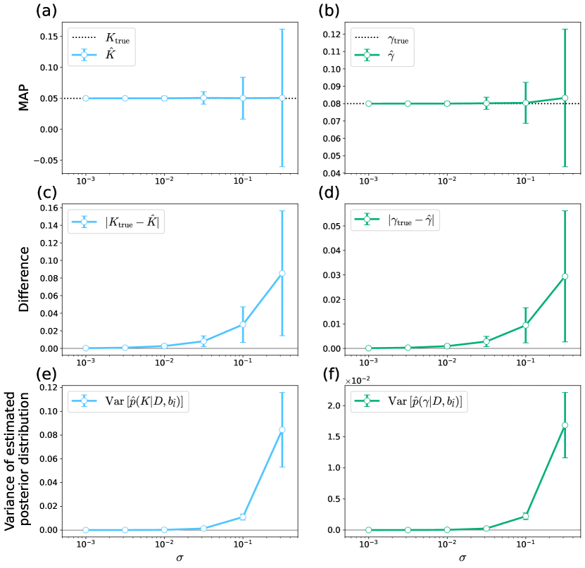
In Figs. 2 (a) and (b), we plot the mean and standard deviation of MAP estimators derived from multiple EMC simulations. These panels suggest that the estimation results are more likely to fluctuate as we increase the noise intensity, although the mean of multiple MAP estimators is always close to the true value. We show the mean and standard deviation of the differences between MAP estimators and the true value in Figs. 2 (c) and (d), which also suggest the improved estimation accuracy for smaller noise intensities.
To compare the shape of posterior distributions, we calculate the variances of the Monte-Carlo samplings from -th replica, which corresponds to the variances of the estimated posterior distributions and , for each EMC simulation. Then, we plot the mean and standard deviation of the variances in Figs. 2 (e) and (f). According to these panels, we can confirm that the posterior distribution becomes sharper for smaller values of . We also find that, as the noise increases, the variances of posterior distributions are likely to fluctuate.
III.3 Estimation from data generated by Kuramoto model
Here, we infer the model parameters using the time series data generated from the Kuramoto model (1) with the Lorentzian distribution of natural frequencies [Eq. (3)]. When creating the time series of the order parameter, we numerically integrate Eq. (1) by the fourth-order Runge-Kutta method with the time step and calculate the Kuramoto order parameter for each data point. For the initial condition, we fix for all , which corresponds to .
In Fig. 3, we present the estimation results for three different datasets. The time series data used in columns (A), (B), and (C) are generated from Eq. (1) with , , and , respectively. The datasets are shown as scatter plots in the first row of Fig. 3 [panels (A-1), (B-1) and (C-1)], with the exact solution . For each dataset, we perform the EMC simulation once. In the second row, we plot the Bayesian free energy against inverse temperatures . The dotted vertical lines represent the inferred inverse temperature . The optimal replica index is described in the upper right of each panel. In the third and fourth rows, we show the histograms of the Monte-Carlo samplings from -th replica, with respect to and , respectively. These histograms correspond to the estimates of posterior distributions. The solid and dotted vertical lines denote the true value and the MAP estimator for each parameter (i.e., and ), respectively. The values of and are shown in the upper right of each panel. The fifth row represents the two-dimensional histograms, which are the estimates of posterior distributions in the two-dimensional parameter space. The black dotted lines show the true values of and .
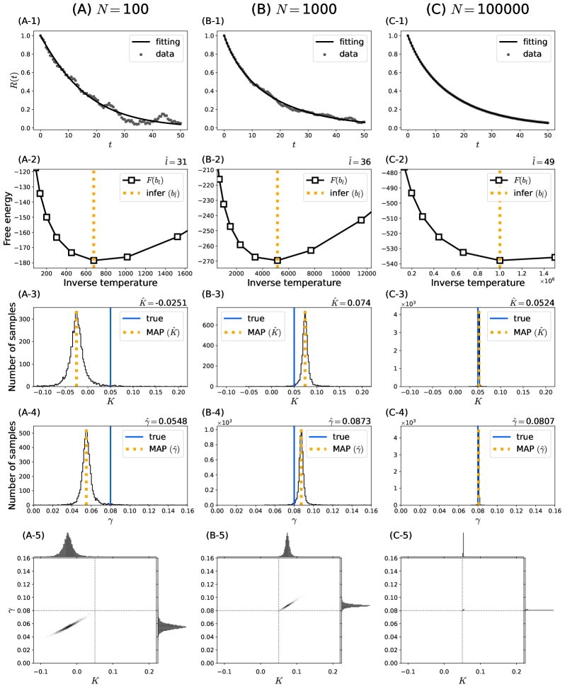
Figure 3 suggests that the estimated parameters () become closer to the true values for larger values of . We also find that the dispersion of the histograms (posterior distribution) varies depending on the value of . To quantitatively examine how the oscillator number affects the estimation, we compare the results of multiple EMC simulations for five different values of (Fig. 4). In this figure, we create 1000 different data sets from Eq. 1 for each oscillator number and perform EMC for each dataset. We calculate several statistical quantities for each oscillator number and compare the results.

Figures 4 (a) and (b) show the mean and standard deviation of multiple MAP estimators for each oscillator number . These panels suggest the increased accuracy and decreased fluctuation of MAP estimators for the larger value of . In contrast to Figs. 2 (a) and (b), where MAP estimators for large fluctuate both above and below the true parameter values, we observe that MAP estimators for small exhibit a bias toward larger values than the true values. In Figs. 4 (c) and (d), we show the mean and standard deviation of the differences between MAP estimators and the true values, which suggests that the estimation becomes accurate as we increase . In Figs. 4 (e) and (f), we compare the variances of estimated posterior distributions [ and , respectively] for different values of . We calculate the variance of the Monte-Carlo samplings from -th replica for each EMC simulation and plot the mean and standard deviation of the variances. We see that the posterior distribution becomes sharper and less diverse (i.e., smaller fluctuation in the variances of the posterior distribution) for larger values of .
Of note, the random number seeds for generating data sets in Figs. 1 and 3 are determined based on the results of multiple EMC simulations shown in Figs. 2 and 4, respectively. We choose the data sets in Figs. 1 and 3 so that the difference between the inferred MAP estimator and true value is closest to the mean of that among multiple EMC simulations with corresponding or in Figs. 2 and 4 [the white dot in panels (c) and (d) of these two figures]. For more details about the simulation codes, see our GitHub repository described in Data Availability section.
IV Discussion and conclusion
In this study, we propose a Bayesian framework for estimating the parameters of the Kuramoto model from the time series data of the order parameter and investigate the estimation accuracy of our approach through numerical experiments. We first confirm the validity of our framework by adopting the same model for both data generation and estimation, and then we examine the finite size effect of the number of oscillators by using the Kuramoto model (1) for data generation. Figures 1 and 2 show that the estimation is accurate when the observational noise intensity is small (e.g., ), suggesting that the exchange Monte Carlo algorithm is correctly implemented in our framework. According to Figs. 3 and 4, we also find that our estimation is accurate if the system size is sufficiently large.
One of the limitations of our approach is the decreased estimation accuracy in the small system size (Figs. 3 and 4), which is likely to be due to the finite size effect [9]. A possible approach to improve estimation accuracy is to change the property of observation noise from the current white Gaussian noise [in Eq. (8)] to another random variable with a time correlation. Namely, instead of Eq. (8), we can use the following model for estimation:
| (32) |
where is a time-correlated random variable (e.g., Brownian motion). Since the difference between the trajectory of Eq. (1) and its approximation (28) at depends on the difference at the previous time point (), we expect that we can better estimate the parameters of the Kuramoto model with smaller if we use Eq. (32).
As we describe in Sec. II.2.4, the marginal likelihood can be accurately calculated by using the EMC method. Since the marginal likelihood represents the validity of the model, we can expand our estimation framework to compare multiple coupled oscillator models. For example, we can also consider the Sakaguchi-Kuramoto model [40], which is a generalization of the Kuramoto model (1) with an additional parameter that denotes the phase shift. By comparing the marginal likelihood of the Kuramoto model (1) and the Sakaguchi-Kuramoto model, we can estimate which model is more likely for a given dataset. Model comparison is an important future direction, which can be especially useful when selecting an appropriate model based on experimental data.
In conclusion, by using the theoretical results from Ott-Antonsen ansatz, we estimate the model parameters from macroscopic observations. We adopt the EMC method to estimate the parameters of the Kuramoto model, which is, to the best of our knowledge, the first attempt in the field of nonlinear oscillators. The estimation is accurate for small observational noise intensity and large system size. Addressing the reduced estimation accuracy due to finite size effects and expanding our framework for model comparison remain significant future challenges.
Data avairability
The data and simulation codes used in the present article are available in the following GitHub repository: https://github.com/yuu-kato/EMC_kuramoto_2025.
Acknowledgements.
Y.K. thanks H. Ishii and J. Albrecht for the technical advice on the EMC simulation codes and valuable discussion, in particular the idea of using Brownian motion for the observational noise term. Y.K. also thanks R. Großmann, C. Beta, O. Omelchenko, M. Rosenblum, T. Carletti, and M. Moriamé for fruitful discussion. This study was supported by the JSPS KAKENHI (No. JP23H00486) to M.O., the JSPS KAKENHI (No. JP23KJ0756) to Y.K., the JSPS KAKENHI (No. JP23KJ0723) to S.K., the JSPS KAKENHI (No. JP21J23250) to E.W., and the Graduate School of Frontier Sciences, The University of Tokyo, through the Challenging New Area Doctoral Research Grant (Project No. C2407) to Y.K and S.K.Author contributions
Y.K., S.K., E.W., M.O., and H.K. conceived this project and discussed the research direction. S.K. provided the original codes for the EMC estimation and its visualization. Y.K. revised the simulation codes with support from S.K. Y.K. performed the numerical experiments and created the figures in this article. Y.K. wrote the manuscript with the input from the rest of the authors. All authors confirmed the final version of the manuscript. M.O. and H.K. supervised the project.
Appendix A Optimization of inverse temperature by hierarchical Bayes approach
According to the hierarchical Bayes approach, the posterior distribution of is calculated as
| (33) |
In the last equation, we assume that the prior density of is subject to a discrete uniform distribution, i.e., . Note that the value of that maximizes the posterior density Eq. (33) coincides with given by Eq. (23) in this case.
References
- Pikovsky et al. [2002] A. Pikovsky, M. Rosenblum, and J. Kurths, Synchronization: a universal concept in nonlinear science (Cambridge University Press, 2002).
- Smith [1935] H. M. Smith, Synchronous flashing of fireflies, Science 82, 151 (1935).
- Uhlhaas and Singer [2006] P. J. Uhlhaas and W. Singer, Neural synchrony in brain disorders: relevance for cognitive dysfunctions and pathophysiology, Neuron 52, 155 (2006).
- Hammond et al. [2007] C. Hammond, H. Bergman, and P. Brown, Pathological synchronization in Parkinson’s disease: networks, models and treatments, Trends in Neurosciences 30, 357 (2007).
- Jiruska et al. [2013] P. Jiruska, M. De Curtis, J. G. Jefferys, C. A. Schevon, S. J. Schiff, and K. Schindler, Synchronization and desynchronization in epilepsy: controversies and hypotheses, The Journal of Physiology 591, 787 (2013).
- Strogatz et al. [2005] S. H. Strogatz, D. M. Abrams, A. McRobie, B. Eckhardt, and E. Ott, Crowd synchrony on the millennium bridge, Nature 438, 43 (2005).
- Kuramoto [1984] Y. Kuramoto, Chemical Oscillations, Waves, and Turbulence (Springer, New York, 1984).
- Acebrón et al. [2005] J. A. Acebrón, L. L. Bonilla, C. J. Pérez Vicente, F. Ritort, and R. Spigler, The Kuramoto model: A simple paradigm for synchronization phenomena, Reviews of Modern Physics 77, 137 (2005).
- Rodrigues et al. [2016] F. A. Rodrigues, T. K. D. Peron, P. Ji, and J. Kurths, The Kuramoto model in complex networks, Physics Reports 610, 1 (2016).
- Pietras and Daffertshofer [2019] B. Pietras and A. Daffertshofer, Network dynamics of coupled oscillators and phase reduction techniques, Physics Reports 819, 1 (2019).
- Cumin and Unsworth [2007] D. Cumin and C. Unsworth, Generalising the Kuramoto model for the study of neuronal synchronisation in the brain, Physica D: Nonlinear Phenomena 226, 181 (2007).
- Filatrella et al. [2008] G. Filatrella, A. H. Nielsen, and N. F. Pedersen, Analysis of a power grid using a Kuramoto-like model, The European Physical Journal B 61, 485 (2008).
- Potratzki et al. [2024] M. Potratzki, T. Bröhl, T. Rings, and K. Lehnertz, Synchronization dynamics of phase oscillators on power grid models, Chaos: An Interdisciplinary Journal of Nonlinear Science 34 (2024).
- Wang and Roychowdhury [2017] T. Wang and J. Roychowdhury, Oscillator-based ising machine, arXiv preprint arXiv:1709.08102 (2017).
- Smelyanskiy et al. [2005] V. Smelyanskiy, D. G. Luchinsky, D. Timucin, and A. Bandrivskyy, Reconstruction of stochastic nonlinear dynamical models from trajectory measurements, Physical Review E 72, 026202 (2005).
- Stankovski et al. [2015] T. Stankovski, V. Ticcinelli, P. V. McClintock, and A. Stefanovska, Coupling functions in networks of oscillators, New Journal of Physics 17, 035002 (2015).
- Stankovski et al. [2017] T. Stankovski, T. Pereira, P. V. McClintock, and A. Stefanovska, Coupling functions: universal insights into dynamical interaction mechanisms, Reviews of Modern Physics 89, 045001 (2017).
- Tokuda et al. [2019] I. T. Tokuda, Z. Levnajic, and K. Ishimura, A practical method for estimating coupling functions in complex dynamical systems, Philosophical Transactions of the Royal Society A 377, 20190015 (2019).
- Ozawa and Kori [2024] A. Ozawa and H. Kori, Two distinct transitions in a population of coupled oscillators with turnover: desynchronization and stochastic oscillation quenching, Physical Review Letters 133, 047201 (2024).
- Ott and Antonsen [2008] E. Ott and T. M. Antonsen, Low dimensional behavior of large systems of globally coupled oscillators, Chaos: An Interdisciplinary Journal of Nonlinear Science 18, 037113 (2008).
- Ott and Antonsen [2009] E. Ott and T. M. Antonsen, Long time evolution of phase oscillator systems, Chaos: An interdisciplinary Journal of Nonlinear Science 19 (2009).
- Yamaguchi and Terada [2024] Y. Y. Yamaguchi and Y. Terada, Reconstruction of phase dynamics from macroscopic observations based on linear and nonlinear response theories, Physical Review E 109, 024217 (2024).
- Daido [1992] H. Daido, Order function and macroscopic mutual entrainment in uniformly coupled limit-cycle oscillators, Progress of Theoretical Physics 88, 1213 (1992).
- Hukushima and Nemoto [1996] K. Hukushima and K. Nemoto, Exchange Monte Carlo method and application to spin glass simulations, Journal of the Physical Society of Japan 65, 1604 (1996).
- Nagata et al. [2012] K. Nagata, S. Sugita, and M. Okada, Bayesian spectral deconvolution with the exchange Monte Carlo method, Neural Networks 28, 82 (2012).
- Tokuda et al. [2017] S. Tokuda, K. Nagata, and M. Okada, Simultaneous estimation of noise variance and number of peaks in Bayesian spectral deconvolution, Journal of the Physical Society of Japan 86, 024001 (2017).
- Kashiwamura et al. [2022] S. Kashiwamura, S. Katakami, R. Yamagami, K. Iwamitsu, H. Kumazoe, K. Nagata, T. Okajima, I. Akai, and M. Okada, Bayesian spectral deconvolution of X-ray absorption near edge structure discriminating between high-and low-energy domains, Journal of the Physical Society of Japan 91, 074009 (2022).
- Ueda et al. [2023] H. Ueda, S. Katakami, S. Yoshida, T. Koyama, Y. Nakai, T. Mito, M. Mizumaki, and M. Okada, Bayesian approach to t 1 analysis in nmr spectroscopy with applications to solid state physics, Journal of the Physical Society of Japan 92, 054002 (2023).
- Kashiwamura et al. [2024] S. Kashiwamura, S. Katakami, T. Yamasaki, K. Iwamitsu, H. Kumazoe, K. Nagata, T. Okajima, I. Akai, and M. Okada, Noise-robust analysis of x-ray absorption near-edge structure based on poisson distribution, Science and Technology of Advanced Materials: Methods 4, 2397939 (2024).
- Yanagita and Mikhailov [2010] T. Yanagita and A. S. Mikhailov, Design of easily synchronizable oscillator networks using the Monte Carlo optimization method, Physical Review E 81, 056204 (2010).
- Iwamitsu et al. [2021] K. Iwamitsu, Y. Nishi, T. Yamasaki, M. Kamezaki, K. Higashiyama, S. Yakura, H. Kumazoe, S. Aihara, K. Nagata, M. Okada, et al., Replica-exchange Monte Carlo method incorporating auto-tuning algorithm based on acceptance ratios for effective Bayesian spectroscopy, Journal of the Physical Society of Japan 90, 104004 (2021).
- Metropolis et al. [1953] N. Metropolis, A. W. Rosenbluth, M. N. Rosenbluth, A. H. Teller, and E. Teller, Equation of state calculations by fast computing machines, The Journal of Chemical Physics 21, 1087 (1953).
- Nagata and Watanabe [2008] K. Nagata and S. Watanabe, Asymptotic behavior of exchange ratio in exchange Monte Carlo method, Neural Networks 21, 980 (2008).
- Bishop and Nasrabadi [2006] C. M. Bishop and N. M. Nasrabadi, Pattern recognition and machine learning (Springer, 2006) p. 555.
- Bernardo and Smith [1994] J. M. Bernardo and A. F. Smith, Bayesian theory (John Wiley & Sons, 1994).
- Gelman et al. [2013] A. Gelman, J. B. Carlin, H. S. Stern, and D. B. Rubin, Bayesian data analysis, 3rd ed. (Chapman and Hall/CRC, 2013).
- Wenden et al. [2012] B. Wenden, D. L. Toner, S. K. Hodge, R. Grima, and A. J. Millar, Spontaneous spatiotemporal waves of gene expression from biological clocks in the leaf, Proceedings of the National Academy of Sciences 109, 6757 (2012).
- Muranaka and Oyama [2016] T. Muranaka and T. Oyama, Heterogeneity of cellular circadian clocks in intact plants and its correction under light-dark cycles, Science Advances 2, e1600500 (2016).
- Watanabe et al. [2023] E. Watanabe, T. Muranaka, S. Nakamura, M. Isoda, Y. Horikawa, T. Aiso, S. Ito, and T. Oyama, A non-cell-autonomous circadian rhythm of bioluminescence reporter activities in individual duckweed cells, Plant Physiology 193, 677 (2023).
- Sakaguchi and Kuramoto [1986] H. Sakaguchi and Y. Kuramoto, A soluble active rotater model showing phase transitions via mutual entertainment, Progress of Theoretical Physics 76, 576 (1986).