Inhomogeneous model with a space dependent Cosmological Constant

Abstract

We analyse an inhomogeneous cosmological model featuring a spherically symmetric bubble solution induced by a unified single perfect fluid, comprising spatially dependent Dark Energy (with $w=-1$) and Dark Matter (with $w=0$) components. We impose an Hubble profile that matches the Planck value at early times ($H_{0}=67.4\pm 0.5$ Km/s Mpc) and the local value (${\cal H}_{0}=73.52\pm 1.62$ Km/s Mpc). We explicitly derive perturbative solutions in two distinct regimes: one expanded around the center (for small $r\,{\cal H}_{0}\ll 1$) and the other expanded around a homogeneous FRW universe. In both cases, we compute the cosmographic parameters, redshift profiles for the Hubbles expansion rates, and effective equations of state. Furthermore, we investigate the redshift drift behaviour extended to a Lema$\hat{\rm i}$tre metric.

1 Introduction

With the discovery of an accelerated expansion of the universe, cosmology entered into the Dark Energy (DE) era [1]. The introduction of a Cosmological Constant (CC) inside the Einstein eqs is the simplest resolution to explain the main features of the present data. However, with the advent of more observations some tensions have energed. In particular, the $H_{0}$-tension problem arises because, while the CMB Planck data yields a value for the Hubble constant $H_{0}=67.4\pm 0.5\,Km/s/Mpc$ within the $\Lambda CDM$ model [2], local measurements favour higher values, such as ${\cal H}_{0}=73.52\pm 1.62\,Km/s/Mpc$ [3]. The explanation of this discrepancy has led to a significant number of studies (see [4] and [5] as general reviews). In a recent paper [6], we discussed an alternative proposal that can be categorized, following the classification of [4], as a solution under the chapter Local Inhomogeneity, representing a viable alternative for late-time evolution. In this study, we move away from the homogeneous space-time typically characterized by FRW backgrounds [8] and instead focus on a spherical void model [9] generated by a unified single perfect fluid that behaves as both Dark Matter (DM) and Dark Energy (DE). While spherical models containing only DM belong to the class of Lemaitre-Tolman-Bondi (LTB) models [10], [11], the inclusion of a DE (radially dependent) component has not been previously studied. The main geometrical difference from the LTB models is the presence of a spatial gradient in the pressure ([12], [13], [14]), which induces acceleration for comoving observers. In a series of papers ([6], [7]), we studied a Lagrangian model generating a perfect fluid where the DE component is linked to the thermodynamic intrinsic entropy of the fluid, conserved over time but space-dependent. In the present work, we omit the detailed theoretical structure of such a models and focus on a single Perfect Fluid (PF) system, where the energy density $\rho(t,r)$ is the sum of a space-dependent CC $\Lambda(r)$ and a DM component proportional to the conserved density $n(t,r)$. The pressure $p(r)$ has only the negative DE contribution:

$$\rho(t,r)=\Lambda(r)+m\,n(t,r),\quad p(r)=-\Lambda(r)$$ (1.1)

where $m$ is a mass parameter that we can absorb into $n$, so we set $m=1$.
We stress that such a system is a single fluid, meaning that its energy-momentum tensor (EMT) follows a single conservation law that unifies the two components (DM and DE) (see (2.7)). In most cases, the EMTs of DM and DE follow separate conservation laws. We study this simple system by solving its evolution equations using two different approximations.
In the first approximation (Chapter 5), we expand the Einstein eqs for small values of $r\,{\cal H}_{0}$ values and we obtain solutions for the nearby central region.
In the second approximation (Chapter 6), we expand around a FRW solution, i.e., we treat small deviations (dependent on $r$) from the constant values of the CC energy density ($\rho_{\Lambda}=const$) and from the DM density ($a(t)^{3}\,n_{DM}=const$) (where scale factor $a(t)$ satisfies eq. (6.4)).
Finally, in Chapter 3, we analyse the past light geodesic eqs, defining various observables in the redshift space.
Moreover, in Chapter 4, we study the bubble’s imprint on the redshift drift, improving its definition within the context of a Lema$\hat{\rm i}$tre metric.
A drawback of this approach is the breaking of the homogeneity. The presence of a center implies that off-center observers would perceive an anisotropic universe [15]. For example, the CMB dipole provides stringent bounds, allowing at most a displacement of 15 Mpc from the center of the underdense bubble [11], [15], [16], [17] (a larger estimate is possible once our peculiar motion cancels part of the dipole). In our case, following [10], we reevaluate the fine tuning required, taking into account the peculiar velocity of an observer at the comoving coordinate $r=d$ relative to the symmetry center:

$$v(d)=d\;\left({\cal H}_{0}-{\cal H}_{0}(d)\right),\qquad{\cal H}_{0}={H}_{0}+\Delta H_{0},\;\;{\cal H}_{0}(r)={H}_{0}+\Delta H_{0}\,e^{-r^{2}/\Delta^{2}}$$ (1.2)

see (6.19, 6.24), this uses the deviation from the Hubble law. Taking as an order of magnitude the CMB dipole velocity $v\sim 10^{-3}$, we obtain

$$d\sim\sqrt[3]{\frac{\Delta^{2}}{\Delta H_{0}}\;v}\sim 3.67\;\left(\frac{\Delta}{Mpc}\right)^{2/3}Mpc\sim 990\;\Re^{2/3}\,Mpc,\qquad\Delta\equiv\frac{\Re}{H_{0}}$$ (1.3)

This is a non-negligible fraction of the inhomogeneity, with $d/\Delta\sim 0.48$, improving the constraints from fine-tuning considerations. A similar result is obtained in [10], where the Hubble profile is $H_{0}+\Delta H_{0}\,e^{-r/\Delta}$.

2 Lema$\hat{\rm i}$tre spacetime metric

A generic spherically symmetric spacetime can be described, using comoving coordinate, by the following Lema$\hat{\rm i}$tre metric [14], [18], [19]

$$ds^{2}=-F^{2}(t,r)\;dt^{2}+X^{2}(t,r)\;dr^{2}+R^{2}(t,r)\;(\;d\theta^{2}+\sin(\theta)\;d\phi^{2})$$ (2.1)

The matter flow has 4-velocity $u^{\alpha}=(1/F,\;0,\;0,\;0)$, while the orthogonal space like 4-vector is $v^{\alpha}=(0,\;1/X,\;0,\;0)$. There are generically two covariant derivatives for a scalar function $f(t,r)$, one along the fluid flow lines $u^{\alpha}$ and one along the preferred space-like direction $v^{\alpha}$:

$$\frac{df}{d\tau}\equiv\dot{f}\equiv u^{\alpha}\nabla_{\alpha}\,f=\frac{f^{(1,0)}}{F},\qquad\frac{df}{d\mathfrak{r}}\equiv\hat{f}\equiv v^{\alpha}\nabla_{\alpha}\,f=\frac{f^{(0,1)}}{X}$$ (2.2)

where $d\tau=F\,dt$ and $d\mathfrak{r}=X\,dr$. Note also that in many articles the $X(t,r)$ function is parametrised as

$$X(t,r)\equiv\frac{R^{(0,1)}(t,r)}{\sqrt{1+E(t,r)}}\;\to\;E=\hat{R}^{2}-1$$ (2.3)

where the $E$ function ($E>-1$) is the curvature parameter [20]. The geometrical quantities derived from the gradient of the 4-velocity matter field for a Locally Rotationally Symmetric (LRS) spacetime are presented in Appendix (A). The expressions for the acceleration ${\cal A}$, shear $\Sigma$, and expansion $\theta$, using the metric (2.1), result

$${\cal A}=\frac{\hat{F}}{F},\qquad\Sigma=\frac{2}{3}\left(\frac{\dot{X}}{X}-\frac{\dot{R}}{R}\right),\qquad\theta=\left(\frac{\dot{X}}{X}+2\;\frac{\dot{R}}{R}\right)$$ (2.4)

The energy momentum tensor (EMT) of our system is that of a PF

$$T_{\mu\nu}=(p+\rho)\;u_{\mu}\;u_{\nu}+p\;g_{\mu\nu}$$ (2.5)

where density and pressure are given by

$$\rho(t,r)=\Lambda(r)+n(t,r),\quad p(r)=-\Lambda(r)$$ (2.6)

The key point about such a fluid is the fact that the EMT is not the sum of two separately conserved components

$$T^{(DE)}_{\mu\nu}=\Lambda\,g_{\mu\nu},\quad T^{(DM)}_{\mu\nu}=n\,u_{m}\,u_{\nu},\quad\nabla^{\mu}T^{(DE)}_{\mu\nu}\neq 0,\;\;\nabla^{\mu}T^{(DM)}_{\mu\nu}\neq 0,$$ (2.7)

$${\rm but}\quad\nabla^{\mu}\left(T^{(DE)}_{\mu\nu}+T^{(DM)}_{\mu\nu}\right)=0,$$

This implies that DE and DM are strongly coupled, forming a single fluid component.
Our goal is to derive a closed equation for the $R(t,r)$ function. Energy density conservation is linked to the conservation of density $n$ and to the time constancy of the CC

$$\dot{n}+\theta\;n=0\quad\oplus\quad\dot{\Lambda}=0\quad\leftrightarrow\quad\dot{\rho}+\theta\;(\rho+p)=0$$ (2.8)

The eq. for the density can be easily integrated

$$n(t,r)=\frac{{\bf n}(r)}{V[t,r]}=\frac{{\bf n}(r)}{X(t,r)\;R(t,r)^{2}},\qquad\theta=\frac{\dot{V}}{V}$$ (2.9)

where ${\bf n}(r)$ is an arbitrary spatial function (boundary condition). The second eq. for the CC gives $\Lambda\equiv\Lambda(r)$ (again a spatial boundary condition). Finally, the space component of the EMT conservation, $h^{\nu}_{\mu}\nabla^{\lambda}T_{\lambda\nu}=0$, results

$$h^{\nu}_{\mu}\nabla_{\nu}p\equiv D_{\mu}p=-(\rho+p)\;{\cal A}_{\mu}\to D_{\mu}\Lambda=n\;{\cal A}_{\mu},\qquad h^{\nu}_{\mu}=\delta^{\nu}_{\mu}+u^{\nu}\,u_{\mu}$$ (2.10)

where we see that a space-dependent CC induces an acceleration ${\cal A}_{\mu}$ for the comoving observers. Now we introduce the Misner-Sharp mass [18]

$$M(t,r)\equiv\frac{R}{2}\;\left(1+\dot{R}^{2}-\hat{R}^{2}\right)=\frac{R}{2}\;\left(\dot{R}^{2}-E\right)$$ (2.11)

which, in the Newtonian limit, represents the mass inside a shell of radial coordinate $r$. Using the $M(t,r)$ function, the Einstein eqs read

$$\rho=\Lambda+n=2\;\frac{\hat{M}}{R^{2}\;\hat{R}},\qquad-p=\Lambda=2\;\frac{\dot{M}}{R^{2}\;\dot{R}}$$ (2.12)

Note that a curvature singularity ($\rho\to\infty$), called shell crossing, occurs for $\hat{R}\to 0$, unless $\hat{M}\to 0$. This is not the case for our functional choices. The pressure equation can be integrated, yielding

$$M=\frac{1}{6}\;\left(\Lambda\;R^{3}\;+\mathbf{m}(r)\right)$$ (2.13)

where $\mathbf{m}\equiv\mathbf{m}(r)$ is another spatial boundary condition. Inserting (2.13) in (2.11), we define the transverse Hubble expansion rate (i.e. the rate corresponding to the angular directions) ${\cal H}_{\perp}$, which is related to the time derivative of $R$ as:

$${\cal H}_{\perp}^{2}\equiv\frac{\theta}{3}-\frac{\Sigma}{2}=\left(\frac{\dot{R}}{R}\right)^{2} = \left(\frac{R^{(1,0)}}{F\;R}\right)^{2}=\frac{1}{3}\,\left(\Lambda+\frac{\bf m}{R^{3}}+\frac{3\;E}{R^{2}}\right)$$ (2.14)

while the radial derivative of $R$, using the expression for the energy density (2.12) and the density (2.9), can be written as

$$\hat{R}=\frac{X}{3\;{\bf n}}\;\left(\hat{\bf m}+\hat{\Lambda}\;R^{3}\right)=\frac{1}{3\;{\bf n}}\;\left({\bf m}^{\prime}+{\Lambda}^{\prime}\;R^{3}\right)\equiv\sqrt{E(t,r)+1}$$ (2.15)

The same expression can be used also to relate $n$ and $\bf{m}$ as

$$\hat{\bf{m}}=n\;R^{2}\;\left(3\;\hat{R}-\frac{\hat{F}}{F}\;R\right)$$ (2.16)

At this point, we have three arbitrary space-dependent functions ${\bf n},\;{\bf m},\;{\Lambda}$ and the following system of eqs for $F$, $R$, and $X$ :

$$\frac{\hat{F}}{F}=\frac{3\,\hat{\Lambda}\;R^{2}\,\hat{R}}{\hat{\bf m}+\hat{\Lambda}\,R^{3}}\to\boxed{\frac{F^{(0,1)}}{F}=\frac{3\;\Lambda^{\prime}\;R^{2}\;R^{(0,1)}}{\mathbf{m}^{\prime}+\Lambda^{\prime}\;R^{3}}}$$ (2.17)

$${\cal H}_{\perp}^{2}\equiv\left(\frac{\dot{R}}{R}\right)^{2}=\boxed{\left(\frac{R^{(1,0)}}{F\;R}\right)^{2}=\frac{1}{3}\;\left(\!\!\underbrace{\Lambda}_{DE}\!\!+\underbrace{\frac{\bf m}{R^{3}}}_{DM}\!\!+\underbrace{\frac{3\;E}{R^{2}}}_{Curvature}\right)}$$ (2.18)

$$X=\frac{3\,{\bf n}\;R^{(0,1)}}{\Lambda^{\prime}\,R^{3}+{\bf m}^{\prime}}$$ (2.19)

We can introduce also the longitudinal Hubble expansion rate ${\cal H}_{\parallel}$ (i.e. the observed radial Hubble rate connected to the line of sight expansion) [21] given by

$${\cal H}_{\parallel}\equiv\frac{\theta}{3}+\Sigma-{\cal A}=\frac{\dot{X}}{X}-\frac{\hat{F}}{F}=\frac{X^{(1,0)}-F^{(0,1)}}{F\,X}$$ (2.20)

Finally, we have also the volume expansion rate [9] given by

$${\cal H}_{\theta}=\frac{\theta}{3}=\frac{{\cal H}_{\parallel}+2\,{\cal H}_{\perp}+{\cal A}}{3}=\frac{1}{3}\left(\frac{\dot{X}}{X}+2\,\frac{\dot{R}}{R}\right)=\frac{1}{3\,F}\left(\frac{X^{(1,0)}}{X}+2\,\frac{R^{(1,0)}}{R}\right)$$ (2.21)

Using the kinematical variable (2.4), we observe that the shear $\Sigma$ and the acceleration ${\cal A}$ are related to different Hubble expansion rates by

$$\Sigma=2\,({\cal H}_{\theta}-{\cal H}_{\perp}),\quad{\cal A}=3\,{\cal H}_{\theta}-2\,{\cal H}_{\perp}-{\cal H}_{\parallel}$$ (2.22)

To simplify the computations we define the space combination

$${\bf E}(r)\equiv\left(\frac{{\bf m}^{\prime}}{3\,{\bf n}}\right)^{2}-1$$ (2.23)

so that our free spatial functions are now ${\Lambda},\,{\bf m},\,{\bf E}$ (instead of $\bf n$).
The limit to the LTB and FRW cases is given by:

• LTB: From eq. (2.17), we have $\hat{F}=0$, allowing us to set $F=1$. In eq. (2.15), when $\Lambda^{\prime}\to 0$ (i.e. when $\Lambda$ is constant in both space and time), we obtain the time independent limit $E(t,r)\to{\bf E}(r),$ so that eq. (2.19) becomes

  $$\left.X\right|_{LTB}=\frac{3\,{\bf n}\,R^{(0,1)}}{{\bf m}^{\prime}}=\frac{R^{(0,1)}}{\sqrt{1+{\bf E}(r)}}$$ (2.24)

  This corresponds exactly to the LTB parametrisation with ${\bf E}(r)>-1$ [10].

• FRW : To achieve a spatially homogeneous universe, we require the following conditions:

  $$\!\!\!\!\!\!\Lambda(r)=H_{0}^{2}\;\Omega_{\Lambda},\;\;{\bf m}(r)=H_{0}^{2}\;\Omega_{m}\;r^{3},\;\;{\bf n}(r)=\frac{{\bf m}^{\prime}(r)}{3}=H_{0}^{2}\;\Omega_{m}\;r^{2}\;{\rm and}\;{\bf E}(r)=0$$ (2.25)

  For the functions of the metric, we have $\hat{R}=1,\;\hat{F}=\hat{X}=E=0$, so that only eq. (2.14) remains.

Note that the functions ${\cal H}_{\parallel}$ (2.20), ${\cal H}_{\perp}$ (2.14), and ${\cal H}_{\theta}$ (2.21) in a general Lema$\hat{\rm i}$tre spacetime do not exhibit any functional correlation. However in the LTB and FRW cases, we observe specific relationships between these functions

$${\rm FRW:}\;\;{\cal H}_{\parallel}={\cal H}_{\perp}={\cal H}_{\theta},$$ (2.26)

$${\rm LTB:}\;\;{\cal H}_{\parallel}=\frac{R^{(1,1)}}{R^{(0,1)}}={\cal H}_{\perp}\,\left(1+\frac{\partial_{r}\log{\cal H}_{\perp}}{\partial_{r}\log R}\right),\qquad{\cal H}_{\theta}=\frac{{\cal H}_{\parallel}+2\,{\cal H}_{\perp}}{3}$$

3 Geodesic light equations

The determination of the light paths in a given spacetime are given, in the eikonal approximation, by the irrotational null geodesic eqs [22]

$$\frac{dk^{\alpha}}{d\lambda}=k^{\beta}\,\nabla_{\beta}\,k^{\alpha}=0,\quad k^{\alpha}\,k_{\alpha}=0,\quad\nabla_{[\alpha}k_{\beta]}=0,\quad k^{\mu}\equiv\frac{dx^{\mu}(\lambda)}{d\lambda}$$ (3.1)

where $k^{\mu}$ is the tangent vector to the light path $x^{\mu}(\lambda)$ (a null geodesic) and $\lambda$ is an affine parameter. The $k^{\alpha}$ vector can be further parametrised as [23],[24]

$$k^{\alpha}=E\,(u^{\alpha}+d^{\alpha}),\quad d^{\alpha}\,u_{\alpha}=0,\quad d^{\alpha}\,d_{\alpha}=1$$ (3.4)

where the vector $d^{\mu}$ is the spatial direction of propagation while $E=-u^{\alpha}k_{\alpha}$ is the energy of the photon seen by the committing observer $u^{\alpha}$. We consider an observer ${\cal O}$ located at the center of symmetry, at $r=0$, connected by an ingoing radial null geodesic to a comoving source ${\cal E}$ at $r$. The redshift $z$ is related to the ratio of the energy at the emission point to the the energy at the observation point. In general we can express it as:

$$1+z=\frac{(u\cdot k)_{{\cal E}}}{(u\cdot k)_{{\cal O}}}=\frac{E_{{\cal E}}}{E_{{\cal O}}},\quad(u\cdot k)_{{\cal O},{\cal E}}=\left.\frac{k^{0}(t,r)}{F(t,r)}\right|_{{\cal O},{\cal E}}\!\!\!\!,\;\;(1+z(\lambda))=F(t(\lambda),r(\lambda))\;t^{\prime}(\lambda)$$ (3.5)

Note that while $z$ is an observable quantity, the $\lambda$ parameter is not. To compare with observations, we need the relationship between the two, which is given by the following differential eq:

$$\!\!\!\!\!\!\!\!\!\!\!\!\frac{dE}{d\lambda} = -\frac{d(u^{\alpha}\,k_{\alpha})}{d\lambda}=-k^{\beta}\,k^{\alpha}\nabla_{\beta}\,u_{\alpha}=-E^{2}\;\left(\frac{\theta}{3}+d^{\alpha}\,\sigma_{\alpha\beta}\,d^{\beta}+d^{\alpha}\,{\cal A}_{\alpha}\right)\equiv-E^{2}\;\bar{\cal H}_{\parallel}(E,d^{\alpha})$$ (3.6)

$${\rm for}\;\;E_{\cal O}=1,\quad\frac{dz(\lambda)}{d\lambda}=-(1+z(\lambda))^{2}\;\bar{\cal H}_{\parallel}$$

where $\bar{\cal H}_{\parallel}$ represents the longitudinal Hubble expansion rate in the direction of the light ray. In a LRS model we have the following decomposition along the radial space like vector $v^{\alpha}$ [24] (see A)

$${\cal A}_{\alpha}={\cal A}\,v_{\alpha},\quad\sigma_{\alpha\beta}=\Sigma\,v_{\alpha}\,v_{\beta}$$ (3.7)

then, a further decomposition of the spatial vector $d^{\alpha}$ along $v^{\alpha}$, gives

$$d^{a}=\kappa\;v^{a}+\kappa^{a},\quad v^{a}\,\kappa_{a}=0\quad{\rm and}\quad d^{a}d_{a}=1\rightarrow\kappa_{a}\,\kappa^{a}=1-\kappa^{2}$$ (3.8)

with $\kappa\equiv\cos\xi$ the magnitude of the radial component or also the angle in between the radial direction $v^{\alpha}$ and the propagating photon $d^{\alpha}$ direction [25]. Finally $\kappa^{\alpha}$ is a spatial vector living in a 2-d spherical sheet. Eq. (3.6) translate in

$$\frac{dz}{d\lambda} = -(1+z)^{2}\;\left(\frac{\theta}{3}+\Sigma\,\cos\xi^{2}+{\cal A}\,\cos\xi\right)\equiv-(1+z)^{2}\;\bar{\cal H}_{\parallel}(z,\xi)$$ (3.9)

For a radial incoming photons we have $\cos\xi$= -1 and we find the longitudinal Hubble expansion rate (2.20) [21]

$${\cal H}_{\parallel}(z)\equiv\left(\frac{\theta}{3}+\Sigma-{\cal A}\right)$$ (3.10)

In general, the observer’s 4-vector field $u^{\mu}$ is geodesic, meaning it has zero acceleration. However, in our case, we have ${\cal A}\neq 0$, which means we must retain additional terms that are typically neglected. Eq.(3.9) must be solved together with the rest of the geodesic eqs (3.1), which result in the following relations (2.20)

$$\frac{dt}{dr}=-\frac{X}{F},\qquad\frac{dz}{dr}=(1+z)\,X\,{\cal H}_{\parallel}=(1+z)\,\frac{X^{(1,0)}-F^{(0,1)}}{F}$$ (3.11)

4 Redshift Drift

Another observable related to the redshift is his time variation. The so called Sandage-Loeb effect characterises the change in redshift for a given source over time [26],[27]. Drift signals arise from photons emitted and received by the same comoving objects at spatial coordinate ($r_{\cal E}=r$ and $r_{\cal O}=0$) over time intervals. The time variation of such observables leads to a series of time drift measurements, which can take different forms: position drift, angular drift, and redshift drift. A direct measurement of these effects provides a model independent observation of the evolution of the Hubble flow in our Universe, in contrast to conventional analyses that relay on fitting formulas.
Let us consider two consecutive measurements of the redshift by the observer ${\cal O}$ at two different times, $\tau_{\cal O}$ and $\tau_{\cal O}+\delta\tau_{\cal O}$ (we partially use the notations and the analysis of ref. [28]). From eqs (3.4) and (3.9), we can express the variation of the redshift with respect to the conformal time of the observer as (see also (3.2))

$$\dot{z}|_{\cal O} = \frac{dz}{d\tau_{\cal O}}=\frac{d}{d\tau_{\cal O}}\frac{E_{\cal E}}{E_{\cal O}}=\frac{E_{\cal E}}{E_{\cal O}}\left(\frac{d\tau_{\cal E}}{d\tau_{\cal O}}\,\frac{\dot{E}_{\cal E}}{E_{\cal E}}-\frac{\dot{E}_{\cal O}}{E_{\cal O}}\right)=-E_{\cal E}\,\int^{\lambda_{\cal O}}_{\lambda_{\cal E}}\,\left(\frac{\dot{E}}{E^{2}}\right)^{\prime}\;d\lambda$$ (4.1)

We now define and compute the following directional derivatives of $E$ (3.2) ($E^{\prime},\,\dot{E},\,\hat{E}$) [28]

$${\bf A}\equiv-\left(\frac{E^{\prime}}{E^{3}}\right)^{\prime}=\left(\frac{{\cal H}_{\parallel}}{E}\right)^{\prime}=\Pi-{\bf I}={\cal H}_{\parallel}^{2}+\dot{\cal H}_{\parallel}-\hat{\cal H}_{\parallel}$$ (4.2)

$${\bf I}\equiv\left(\frac{\hat{E}}{E^{2}}\right)^{\prime}=\dot{\cal H}_{\parallel}-\frac{\nabla_{\alpha}E}{E}\,{\cal L}_{\vec{k}}e^{\alpha}=\hat{\cal H}_{\parallel}+{\cal H}_{\parallel}\,{\cal A}$$ (4.3)

$$\Pi\equiv-\left(\frac{\dot{E}}{E^{2}}\right)^{\prime}=\dot{\cal H}_{\parallel}-\frac{\nabla_{\alpha}E}{E}\,{\cal L}_{\vec{k}}u^{\alpha}={\cal H}_{\parallel}^{2}+\dot{\cal H}_{\parallel}+{\cal H}_{\parallel}\;{\cal A}$$ (4.4)

here, ${\cal L}_{\vec{k}}$ is the Lie derivative operator along $k^{\alpha}$. Using eq. (3.3) for $f=E$, we obtain the following relationship

$$E^{\prime}=E\,(\dot{E}-\hat{E})\;\to\;{\bf A}=-\left(\frac{\dot{E}-\hat{E}}{E^{2}}\right)^{\prime}\;\to\;\Pi={\bf A}+{\bf I}$$ (4.5)

After integrating the above expressions, we find the following relationships

$$E_{\cal E}\,\int^{\lambda_{\cal O}}_{\lambda_{\cal E}}{\bf A}\,d\lambda=E_{\cal E}\;\left.\frac{{\cal H}_{\parallel}}{E}\right|^{\lambda_{\cal O}}_{\lambda_{\cal E}}=(1+z)\,{\cal H}_{0}-{\cal H}_{\parallel}(z)$$ (4.6)

$$E_{\cal E}\,\int^{\lambda_{\cal O}}_{\lambda_{\cal E}}\,{\bf I}\,\,d\lambda=E_{\cal E}\,\int^{\lambda_{\cal O}}_{\lambda_{\cal E}}\,\left(\hat{\cal H}_{\parallel}+{\cal H}_{\parallel}\,{\cal A}\right)\,d\lambda=E_{\cal O}\,(1+z)\,\int^{z}_{0}\,\frac{\hat{\cal H}_{\parallel}+{\cal H}_{\parallel}\,{\cal A}}{(1+z^{\prime})^{2}\,{\cal H}_{\parallel}}\,dz^{\prime}$$ (4.7)

and using the fact that

$$\frac{\left(\hat{\cal H}_{\parallel}+{\cal H}_{\parallel}\,{\cal A}\right)}{{\cal H}_{\parallel}}=\frac{\hat{\cal H}_{\parallel}}{{\cal H}_{\parallel}}+\frac{\hat{F}}{F}=\hat{\log}({\cal H}_{\parallel}\,F)=\frac{\partial_{r}\log({\cal H}_{\parallel}\,F)}{X}$$ (4.8)

we obtain our final result (with $E_{\cal O}=1$)

$$\!\!\!\!\!\!\!\dot{z}|_{\cal O} = (1+z)\,{\cal H}_{0}-{\cal H}_{\parallel}(z)+(1+z)\,\int^{\lambda_{\cal O}}_{\lambda_{\cal E}}\,{\bf I}\,d\lambda=$$

$$(1+z)\,{\cal H}_{0}-{\cal H}_{\parallel}(z)+(1+z)\,\int^{z}_{0}\,dz^{\prime}\,\frac{1}{(1+z^{\prime})^{2}}\left.\frac{\partial_{r}\log({\cal H}_{\parallel}\,F)}{X}\right|_{r(z^{\prime}),t(z^{\prime})}=$$

$$(1+z)\,{\cal H}_{0}-\left.\frac{X^{(1,0)}-F^{(0,1)}}{X\,F}\right|_{r(z),t(z)}\!\!\!\!\!\!\!+(1+z)\,\int^{z}_{0}\,dz^{\prime}\,\frac{1}{(1+z^{\prime})^{2}}\left.\frac{\partial_{r}\log(\frac{X^{(1,0)}-F^{(0,1)}}{X})}{X}\right|_{r(z^{\prime}),t(z^{\prime})}$$

This agrees with the results obtained for FRW and LTB spacetimes

• In FRW with $F=1,\,X=a(t),\,{\cal H}_{\parallel}=\frac{\partial_{t}a(t)}{a(t)}$ (from eq. (6.4) and (6.12) we have ${\cal H}_{\parallel}(z)=H(a_{0}(z))\equiv H(z)$) (see eq.(6.4) for the Hubble function in $\Lambda$CDM model) we get [26], [29]

  $$\dot{z}|_{\cal O}^{FRW}=(1+z)\,{H}_{0}-{H}(z)$$ (4.10)

• In LTB with $F=1$ and (2.24), ${\cal H}_{\parallel}=\frac{X^{(1,0)}(t,r)}{X(t,r)}=\frac{R^{(1,1)}(t,r)}{R^{(0,1)}(t,r)}$ we obtain [30], [31],[32], [25]

  $$\!\!\!\!\!\!\!\!\!\!\!\!\!\!\dot{z}|_{\cal O}^{LTB} = (1+z)\,{\cal H}_{0}-{\cal H}_{\parallel}(z)+(1+z)\,\int^{z}_{0}\,dz^{\prime}\,\frac{1}{(1+z^{\prime})^{2}}\left.\frac{\partial_{r}\log({\cal H}_{\parallel})}{X}\right|_{r(z^{\prime}),t(z^{\prime})}=$$ (4.12)

  $$(1+z)\,{\cal H}_{0}-{\cal H}_{\parallel}(z)+(1+z)\,\int_{t(z)}^{t_{0}}\,dt^{\prime}\,\frac{1}{(1+z(t^{\prime},r(t^{\prime})))}\left.\frac{\partial_{r}{\cal H}_{\parallel}}{X}\right|_{t^{\prime},r(t^{\prime})}$$

  that corresponds exactly to eq. (25) of ref [33].

As discussed also in ref. [25] the simplifying local picture of a redshift drift $\dot{z}$ formula dominated by the first two terms to the right of eq. (4) is not a good approximation.

5 Solutions near the center

In this section we use the cosmographic approach that consist in a Taylor expansion in redshift of the main cosmological observables that can be combined with a model independent interpretation of the data analysis [34]. The solution of the eqs of motion (2.17, 2.14, 2.19) around the center at $r=0$ requires an expansion of the background space equation of the following form (where $\hat{r}={\cal H}_{0}\,r$)

$$\Lambda(r)={\cal H}_{0}^{2}\,\left(\lambda_{0}+\frac{\lambda_{2}}{2\,!}\,\hat{r}^{2}+\frac{\lambda_{3}}{3\,!}\,\hat{r}^{3}+\ldots\right),$$ (5.1)

$${\bf m}(r)=\frac{1}{{\cal H}_{0}}\,\left(\frac{{\bf m}_{3}}{3\,!}\,\hat{r}^{3}+\frac{{\bf m}_{4}}{4\,!}\,\hat{r}^{4}+\ldots\right),$$

$${\bf E}(r)=\frac{{\bf e}_{2}}{2\,!}\,\hat{r}^{2}+\frac{{\bf e}_{3}}{3\,!}\,\hat{r}^{3}+\ldots,$$

where all the $\lambda_{i},,{\bf m}_{i},\,{\bf e}_{i}$ parameters are dimensionless. The expanded solutions for the form factors of the metric result:

$$F=1+\frac{3}{4}\,a^{3}\,\hat{r}^{2}\,\Omega_{\chi}+a^{2}\,\hat{r}^{3}\,\left(a\,\text{$\Delta$f}+R_{2}(a)\,\Omega_{\chi}\right)+\ldots$$ (5.2)

$$X=a+\hat{r}\,R_{2}(a)+\frac{\hat{r}^{2}}{2}\,\left(R_{3}(a)-a^{4}\,\Omega_{\chi}-a\,\Omega_{\kappa}\right)+\frac{\hat{r}^{3}}{6}\,X_{3}(a)+\ldots$$ (5.3)

$$R=a\,r\,\left(1+\frac{\hat{r}}{2}\,R_{2}(a)+\frac{\hat{r}^{2}}{6}\,R_{3}(a)\right)+\ldots$$ (5.4)

with $\text{$\Delta$f}\equiv\frac{6\,\lambda_{3}-\mathbf{m}_{4}\,\Omega_{\chi}}{108\,\Omega_{m}}$. At leading order ${\cal O}(r^{0})$, we define

$$\lambda_{0}\equiv 3\,\Omega_{\Lambda},\;\;\lambda_{2}\equiv\frac{9}{2}\,\Omega_{m}\,\Omega_{\chi},\;\;{\bf m}_{3}\equiv 18\,\Omega_{m},\;\;{\bf e}_{2}\equiv 2\,\Omega_{\kappa},\;\;$$ (5.5)

so that we can write the local Hubble flow as

$${\cal H}(a)\equiv\frac{a^{\prime}(t)}{a(t)}=\frac{{\cal H}_{0}}{a^{3/2}}\;\sqrt{\Omega_{m}+a\,\Omega_{\kappa}+a^{3}\,\Omega_{\Lambda}+a^{4}\,\Omega_{\chi}}$$ (5.6)

We can begin by giving physical meaning to some of the parameters. The parameter $\Omega_{\kappa}$, which is proportional to the spatial curvature density, provides information about the local structure of the ${\bf E}$ form factor. The matter density, proportional to $\Omega_{m}$, originates from ${\bf m}$. The DE density, proportional to $\Omega_{\Lambda}$, arises from ${\lambda}$, while an anomalous energy density parameter, $\Omega_{\chi}$, results from the simultaneous presence of $\lambda$ and ${\bf m}$. This energy contribution has a very unusual equation of state, with $w=-4/3$.
At second order the leading time dependent form factor $R_{2}(a)$ satisfy the differential eq

$$R_{2}^{\prime}(a) + \left(\frac{1}{2}\left(\frac{\Omega_{m}}{a^{4}}-\frac{2\,\Omega_{\Lambda}}{a}-3\,\Omega_{\chi}\right)\,R_{2}(a)-\frac{\mathbf{e}_{3}}{6\,a^{2}}-\frac{\mathbf{m}_{4}}{72\,a^{3}}-2\,a\,\text{$\Delta$f}\right)\frac{{\cal H}_{0}^{2}}{\mathcal{H}(a)^{2}}=0$$ (5.7)

with the boundaries (at present time $a=1$) $R_{2}(1)=0$. We do not have to explicitly solve this equation but only evaluate

$$R_{2}^{\prime}(1) = 2\,\text{$\Delta$f}+\frac{\mathbf{m}_{4}}{72}+\frac{\mathbf{e}_{3}}{6}$$ (5.8)

$$R_{2}^{\prime\prime}(1) = \text{$\Delta$f}\,\left(2\,\Omega_{\kappa}+3\,\Omega_{m}-\Omega_{\chi}+4\right)+(12\,\mathbf{e}_{3}+\mathbf{m}_{4})\,\left(\frac{\Omega_{\kappa}}{72}+\frac{\Omega_{m}}{48}-\frac{\Omega_{\chi}}{144}-\frac{1}{36}\right)+\frac{\mathbf{e}_{3}}{6}$$

that are useful for the next eqs. At order three, the next correction $R_{3}(a)$ always evolves with a first order equation (with boundary $R_{3}(1)=0$) but we need only his first derivative value at present time

$$R_{3}^{\prime}(1) = -3\,\text{$\Delta$f}^{2}-\frac{\mathbf{e}_{3}\,\mathbf{m}_{4}}{288}-\frac{\mathbf{e}_{3}^{2}}{48}+\frac{\mathbf{e}_{4}}{8}+\frac{\lambda_{4}}{9\,\Omega_{m}}-\text{$\Delta$f}\,\left(\mathbf{m}_{4}\,\left(\frac{1}{9\Omega_{m}}+\frac{1}{24}\right)+\frac{\mathbf{e}_{3}}{2}\right)+$$ (5.9)

$$\Omega_{\chi}\left(3\,\Omega_{\kappa}+\frac{9\,\Omega_{m}}{4}+\frac{9}{2}\right)+\mathbf{m}_{5}\,\left(\frac{1}{120}-\frac{\Omega_{\chi}}{72\,\Omega_{m}}\right)-\frac{\mathbf{m}_{4}^{2}}{6912}+\frac{3\,\Omega_{\chi}^{2}}{4}$$

The longitudinal and the transverse Hubble rates at first order are given by

$${\cal H}_{\parallel}(a,\,\hat{r})={\cal H}(a)-\hat{r}\left(\frac{3}{2}\,a^{2}\,{\cal H}_{0}\,\Omega_{\chi}+\frac{\mathcal{H}(a)\,\left(R_{2}(a)-a\,R_{2}^{\prime}(a)\right)}{a}\right)$$ (5.10)

$${\cal H}_{\perp}(a,\,\hat{r})={\cal H}(a)\left(1-\hat{r}\frac{\,\left(R_{2}(a)-a\,R_{2}^{\prime}(a)\right)}{a}\right)$$ (5.11)

$${\cal H}_{\theta}(a,\,\hat{r})=\mathcal{H}(a)\,\left(1-\frac{2\,\hat{r}}{3}\,\frac{\left(R_{2}(a)-a\,R_{2}^{\prime}(a)\right)}{a}\right)$$ (5.12)

where we note that always ${\cal H}_{\parallel}(a,\hat{r})\leq{\cal H}_{\perp}(a,\hat{r})$ for $\Omega_{\chi}>0$.

5.1 Observables along the light cone

The perturbative solutions for the light cone geodesic eqs (6.11), for small $z$ values, result [34], [28], [35]

$$a(z)=1-z+z^{2}\,\left(\frac{1}{2}\left(R_{2}^{\prime}(1)+2\right)-\frac{3\,\Omega_{\chi}}{4}\right)+{\cal O}(z^{3})$$ (5.13)

$$r(z)=\frac{z}{{\cal H}_{0}}+\frac{z^{2}}{{\cal H}_{0}}\,\left(\frac{1}{4}\,\left(2\,\Omega_{\Lambda}-\Omega_{m}-2\,R_{2}^{\prime}(1)-2\right)+\frac{3\,\Omega_{\chi}}{2}\right)+{\cal O}(z^{3})$$ (5.14)

Parametrising the small $z$ series of the luminosity distance function, $d_{L}(z)\equiv(1+z)^{2}\,R(a(z),\,r(z))$, in the following way [34]

$$d_{L}(z) \simeq \frac{z}{{\cal H}_{0}}+\frac{z^{2}}{{\cal H}_{0}}\,\frac{\left(1-Q_{0}\right)}{2}-\frac{z^{3}}{{\cal H}_{0}}\,\frac{\left(1-Q_{0}-3\,Q_{0}^{2}+J_{0}\right)}{6}+{\cal O}(z^{4})$$ (5.15)

we get, at first order, the Hubble constant ${\cal H}_{0}$ that we set to come from local measurements [3]: ${\cal H}_{0}=73.52\pm 1.62\,Km/s/Mpc$. At second order we have the $Q_{0}$ deceleration parameter and, at third order, the jerk parameter $J_{0}$. In order to show the effect of the bubble profile, we can factorise out the $\Lambda$CDM contributions ($q_{0}$ and $j_{0}$) writing $Q_{0}\equiv q_{0}+\Delta q,\;J_{0}\equiv j_{0}+\Delta j$ where

$$\!\!\!\!\!\!\!\!\!\!\!\!\!\!\!\Delta q=\Omega_{\kappa}-2\,\Omega_{\chi}+R_{2}^{\prime}(1)$$ (5.20)

$$\!\!\!\!\!\!\!\!\!\!\!\!\!\!\!\Delta j=\frac{17\,\Omega_{\chi}}{2}-6\,\Delta f-2\,\Omega_{\kappa}+R_{2}^{\prime}(1)\,\left(2\,\Omega_{\kappa}+3\,\Omega_{m}-\Omega_{\chi}-1\right)-2\,R_{2}^{\prime\prime}(1)+R_{3}^{\prime}(1)$$

Then we can compute the $z$ series of the Hubble functions ${\cal H}_{i}(z)=H_{\Lambda CDM}(z)+\Delta{\cal H}_{i}(z)$ and also of the effective equations of state ${w}_{i}(z)\equiv w_{\Lambda CDM}(z)+\Delta w_{i}(z)$, $\;i=\parallel,\,\perp,\,\theta$ , see (6.29). For the longitudinal Hubble expansion rate (2.20) we get

$${\cal H}_{\parallel}(z) = {\cal H}_{0}\,\left(1+z\,\left(1+Q_{0}\right)+\frac{z^{2}}{2}\,\left(\Delta q+J_{0}-Q_{0}^{2}\right)\right)$$ (5.23)

$$\Delta{\cal H}_{\parallel}(z)=\left(z\;\,\Delta q+\frac{z^{2}}{2}\;\left(\Delta j-\Delta q^{2}+\Delta q\,(1-2\,q_{0})\right)\right)\,{\cal H}_{0}$$

$$\Delta w_{\parallel}(z)=\frac{2\,\Delta q}{3}+\frac{2}{3}\,z\,\left(\Delta j-2\,\Delta q^{2}-4\,\Delta q\,q_{0}\right)$$

so that a measure of $\Delta{\cal H}_{\parallel}(z)$ and or $\Delta w_{\parallel}$, at leading order in $z$, corresponds to a measure of $\Delta q$. For the transversal functions (2.14) we get

$$\Delta{\cal H}_{\perp}(z)=\Delta{\cal H}_{\parallel}(z)+\left(\frac{3}{2}\,z\,\Omega_{\chi}+z^{2}\;\left(3\,\Delta f-\frac{3}{4}\left(\Delta q-(5+\,q_{0})\right)\,\Omega_{\chi}\right)\right)\,{\cal H}_{0}$$ (5.24)

$$\Delta w_{\perp}(z)=\Delta w_{\parallel}(z)+\Omega_{\chi}+z\,\left(4\,\Delta f-3\,(2+\Delta q+q_{0})\,\Omega_{\chi}-\frac{3}{2}\,\Omega_{\chi}^{2}\right)$$ (5.25)

where we see that a measure of $\Delta{\cal H}_{\perp}(z)$ and/or $\Delta w_{\perp}$, at leading order in $z$, corresponds to a measure of $\Omega_{\chi}$. For the volume Hubble expansion rate (2.14) we get

$$\Delta{\cal H}_{\theta}(z) = {\cal H}_{0}\,z\,\left(\frac{1}{6}\left(2\,\Omega_{\kappa}+5\,\Omega_{\chi}\right)-\frac{\text{$\Delta$q}}{3}\right)+{\cal H}_{0}\,z^{2}\,\left(\frac{5\,\text{$\Delta$f}}{3}+\frac{\text{$\Delta$q}^{2}}{6}+\frac{1}{36}\text{$\Delta$q}\left(-2\,\Omega_{\kappa}+\right.\right.$$

$$\left.\left.+15\,\Omega_{m}-17\,\Omega_{\chi}-20\right)+\frac{1}{72}\left(-8\,\Omega_{\kappa}^{2}-16\,\Delta j+\Omega_{\kappa}\,\left(-30\,\Omega_{m}+20\,\Omega_{\chi}+8\right)-\right.\right.$$

$$\left.\left.\Omega_{\chi}\left(21\,\Omega_{m}+8\,\Omega_{\chi}+88\right)-8\,R_{2}^{\prime\prime}(1)\right)\right)$$

In this case a measure of $\Delta{\cal H}_{\theta}$ is in between $\Delta{\cal H}_{\parallel/\perp}$ being proportional both to $\Omega_{\chi,\kappa}$.
The $z$ expansion of the redshift drift in the $\Lambda$CDM model gives

$$\dot{z}_{\Lambda CDM} = -{\cal H}_{0}\,z\,q_{0}+{\cal O}(z^{2})$$ (5.27)

while in our model we get (the details are given in appendix B) [34]

$$\dot{z} = \dot{z}_{\Lambda CDM}+\Delta\dot{z},\quad\Delta\dot{z}=-{\cal H}_{0}\,z\left(\Omega_{\kappa}+\frac{\Omega_{\chi}}{2}\right)+{\cal O}(z^{2})$$ (5.28)

so that a measurement of $\dot{z}$, together with ${\cal H}_{\perp/\parallel}$, gives a bound on $\Omega_{\kappa}$. From (2.22) we can get the leading terms for shear and acceleration

$$\Sigma=-\frac{2}{3}\,{\cal H}_{0}\,z\,\left(\Delta q-\Omega_{\kappa}+2\,\Omega_{\chi}\right),\quad\mathcal{A}=\,{\cal H}_{0}\,z\,\left(-\Delta q+\Omega_{\kappa}-\frac{\Omega_{\chi}}{2}\right)$$ (5.29)

where we see as the ”anomalous” densities $\Omega_{\chi}$ and $\Omega_{\kappa}$ contribute differently to such a geometrical quantities. From (5.1, 5.24, 5.28) at order ${\cal O}(z)$ we find a consistency relationship in between different observables

$$\left(\Delta{\cal H}_{\theta}-\frac{2}{3}\,\Delta{\cal H}_{\perp}+\frac{1}{3}\Delta\dot{z}\right)_{{\cal O}(z)}=0$$ (5.30)

or equivalently

$$\left(\Delta{w}_{\theta}-\frac{2}{3}\,\Delta{w}_{\perp}\right)_{z=0}+\left(\frac{2}{9\,{\cal H}_{0}}\Delta\dot{z}\right)_{{\cal O}(z)}=0$$ (5.31)

that, in a sense, corresponds to a necessary condition for the model . Experimental observations, in the future, for the equations (5.30) or (5.31) will be an interesting verification activity for the model.

6 Perturbative solution around FRW

In eq. (2.25) we have the parameter space FRW limit of the model. Here we perturb the various form factors of the metric and the space dependent boundary conditions around such a values. For the metric we define the following perturbative structure

$$\!\!\!\!\!\!\!\!F=1+F_{1}+\frac{F_{2}}{2}+...,\;X=a(t)\left(1+X_{1}+\frac{X_{2}}{2}+...\right),\;R=a(t)\,r\,\left(1+R_{1}+\frac{R_{2}}{2}+...\right)$$ (6.1)

While, for the space dependent functions, we introduce different dimensionless perturbations characterised by an index ”1” as $f_{1}$ ($f=\lambda,\,{\bf m},\,{\bf n},\,{\bf e}$)

$${\Lambda}(r)\equiv\Lambda_{0}\,(1+{\lambda}_{1}(r)),\qquad{\bf m}(r)\equiv m_{0}\,r^{3}\,(1+{\bf m}_{1}(r))$$ (6.2)

$${\bf n}(r)\equiv m_{0}\,r^{2}\,(1+{\bf n}_{1}(r)),\quad{\bf E}(r)\equiv{\bf e}_{1}(r)=2\,{\bf m}_{1}(r)+\frac{2}{3}\,r\,{\bf m}_{1}^{\prime}(r)-2\,{\bf n}_{1}(r)$$

To shorten expressions we introduce the notation

$$h(a)\equiv\,_{2}F_{1}\left(\frac{1}{6},1;\frac{2}{3};-\frac{\Omega_{\Lambda}\,a^{3}}{\Omega_{m}}\right)$$ (6.3)

The $a=a(t)$ parameter is the scale factor that satisfies the FRW Hubble time evolution equation

$$H(a)\equiv\frac{a^{\prime}(t)}{a(t)}=H_{0}\;\frac{\sqrt{a(t)^{3}\,\Omega_{\Lambda}+\Omega_{m}}}{a(t)^{3/2}},\qquad\Omega_{\Lambda}+\Omega_{m}=1$$ (6.4)

The solutions of the eqs of motion (2.17, 2.14, 2.19) at first order result

$$\!\!\!F = 1+a^{3}\,\frac{\Omega_{\Lambda}\,\lambda_{1}(r)}{\Omega_{m}}$$ (6.5)

$$\!\!\!X = a\,\left(1+\frac{a\,\mathit{h}(a)\,\left(r\,\mathbf{e}_{1}^{\prime}(r)-\mathbf{e}_{1}(r)\right)}{5\,H_{0}^{2}\,r^{2}\,\Omega_{m}}-\frac{\mathbf{e}_{1}(r)}{2}+\frac{a^{3}\,\Omega_{\Lambda}\,\lambda_{1}(r)}{3\,\Omega_{m}}-\frac{a\,(\mathit{h}(a)-1)\,\lambda_{1}^{\prime\prime}(r)}{3\,H_{0}^{2}\,\Omega_{m}}\right)$$ (6.6)

$$\!\!\!R = a\,r\,\left(1+\frac{a\,\mathit{h}(a)\,\mathbf{e}_{1}(r)}{5\,H_{0}^{2}\,r^{2}\,\Omega_{m}}-\frac{a\,(\mathit{h}(a)-1)\,\lambda_{1}^{\prime}(r)}{3\,H_{0}^{2}\,r\,\Omega_{m}}+\frac{a^{3}\,\Omega_{\Lambda}\,\lambda_{1}(r)}{3\,\Omega_{m}}+\frac{\mathit{m}_{1}(r)}{3}\right)$$ (6.7)

Note that to have regular functions for $r\to 0$, we need at least

$$\frac{\lambda_{1}^{\prime}}{r},\;\;\frac{{\bf e}_{1}}{r^{2}},\;\;\frac{{\bf e}_{1}^{\prime}}{r}\sim finite$$ (6.8)

that requires a small $r$ expansion of the form

$$\lambda_{1}\sim const+\#\,r^{2},\;\;\;{\bf e}_{1}\sim r^{2},\;\;\;\;{\rm i.e.}\;\;\;\;\lambda_{1}^{\prime}(0)=0,\quad\mathbf{e}_{1}(0)=\mathbf{e}_{1}^{\prime}(0)=0$$ (6.9)

The function $\mathbf{m}_{1}(r)$ can be reabsorbed through a radial redefinition (see footnote 3), effectively allowing us to set $\mathbf{m}_{1}(r)=0$ everywhere in (6.2) and (6.5, 6.6, 6.7). Note that, with respect the previous analysis in [6], where only the CC was perturbed, we now have an additional free form factor, ${\bf e}_{1}(r)$, which is proportional to the density perturbations in eqs (6.2).
At infinity, we impose the boundary conditions $\lambda_{1}(r),\,{\bf e}_{1}(r)\to 0$ ensuring that the Hubble function asymptotically approaches the Planck value. The perturbativity of the system is guarantied as long as the following conditions hold:

$$a^{3}\,\lambda_{1}(r),\;a\,\frac{{\lambda}_{1}^{\prime}(r)}{H_{0}^{2}\,r},\;a\,\frac{{\bf e}_{1}(r)}{H_{0}^{2}\,r^{2}},\;a\,\frac{{\bf e}_{1}^{\prime}(r)}{H_{0}^{2}\,r}<1$$ (6.10)

These conditions generally define a closed region in the 2-d spacetime, in the variables $a-r$. However, since $a=1$ at present time, we can safely neglect the time dependence in the above inequalities.

6.1 Redshift equations

In this context the perturbative solutions of the geodesic eqs (3.11) can be obtained making a change of time variable from $t\to a(t)$ where $dt=\frac{da}{a\;H(a)}$. In this way each time derivative has to be substitute with $\partial_{t}f(t,r)=a\,H(a)\,\partial_{a}f(a,r)$ and the system of redshift-geodesic eqs (3.11) becomes

$$\frac{da}{dz}=-\frac{a\;H(a)}{(1+z)\;F\;{\cal H}_{\parallel}},\qquad\frac{dz}{dr}=(1+z)\;X\;{\cal H}_{\parallel},\qquad\frac{da}{dr}=-\frac{a\;H(a)\;X}{F}$$ (6.11)

To treat the above eqs, once we know the functional dependence of the metric (6.5, 6.6, 6.7) and Hubble (2.20), we perturbatively set $a(z)=a_{0}(z)+a_{1}(z)+\dots$ and $\;r(z)=r_{0}(z)+r_{1}(z)+\dots$ and then we solve order by order. At zero order we get the FRW results

$$\!\!\!\!\!\!\!a_{0}(z)=\frac{1}{1+z},\;\;r_{0}(z)=\frac{2}{H_{0}\,\Omega_{m}^{1/2}}\left({}_{2}F_{1}\left(\frac{1}{6},\frac{1}{2};\frac{7}{6};-\frac{\Omega_{\Lambda}}{\Omega_{m}}\right)-\frac{\,{}_{2}F_{1}\left(\frac{1}{6},\frac{1}{2};\frac{7}{6};-\frac{\Omega_{\Lambda}}{(z+1)^{3}\Omega_{m}}\right)}{\sqrt{z+1}}\right)$$ (6.12)

while at first order we obtain the following system of first order differential eqs

$$a_{1}^{\prime}(z) + \frac{a_{1}(z)}{1+z}+\frac{\left(5-3\,h(a_{0})\right)\left(\mathbf{e}_{1}(r_{0})-r_{0}\,\mathbf{e}_{1}^{\prime}(r_{0})\right)}{10\,r_{0}^{2}\,H(a_{0})^{2}}+\frac{\Omega_{\Lambda}\,\left((1+z)\,\lambda^{\prime}(r_{0})-\lambda(r_{0})\,H(a_{0})\right)}{(1+z)^{5}\,\Omega_{m}\,H(a_{0})}+$$ (6.13)

$$\frac{\lambda^{\prime\prime}(r_{0})\,\left(-3\,(1+z)^{3}\,\left(h(a_{0})-1\right)\,\Omega_{m}-2\,\Omega_{\Lambda}\right)}{6\,(1+z)^{3}\,\Omega_{m}\,H(a_{0})^{2}}=0$$

$$r_{1}^{\prime}(z)-\frac{H_{0}^{2}\,(1+z)\,\left((1+z)^{3}\,\Omega_{m}-2\,\Omega_{\Lambda}\right)}{2\,H(a_{0})^{3}}\,a_{1}(z)+\frac{\Omega_{\Lambda}\,\left(\lambda(r_{0})\,H(a_{0})-3\,(1+z)\,\lambda_{1}^{\prime}(r_{0})\right)}{3\,(1+z)^{3}\,\Omega_{m}\,H(a_{0})^{2}}+$$

$$\frac{\lambda_{1}^{\prime\prime}(r_{0})\left((1+z)^{3}\,\left(h(a_{0})-1\right)\,\Omega_{m}-2\,\left(h(a_{0})-2\right)\,\Omega_{\Lambda}\right)}{6\,(1+z)\,\Omega_{m}\,H(a_{0})^{3}}-\frac{\mathbf{e}_{1}(r_{0})}{2\,H(a_{0})}+$$ (6.14)

$$\frac{\left(\mathbf{e}_{1}(r_{0})-r_{0}\,\mathbf{e}_{1}^{\prime}(r_{0})\right)\,\left((1+z)^{3}\,\left(h(a_{0})-5\right)\,\Omega_{m}-2\,h(a_{0})\,\Omega_{\Lambda}\right)}{10\,r_{0}^{2}\,(1+z)\,\Omega_{m}\,H(a_{0})^{3}}=0$$

where $a_{0}=a_{0}(z)$ and $r_{0}=r_{0}(z)$ (see (6.12)) and with initial conditions $a_{1}(0)=r_{1}(0)=0$.

6.2 Hubble functions

Now that we have the perturbative solutions of the Einstein equations and of the geodesic light cone, we can start studying the Hubble functions at first order

$$\!\!\!\!{\cal H}_{\perp}(a,r)^{2} = H(a)^{2}+\left(\frac{\mathit{h}(a)-1}{a^{2}}+\frac{2\,a\,\Omega_{\Lambda}}{3\,\Omega_{m}}\right)\,\frac{\lambda_{1}^{\prime}(r)}{r}+\frac{(5-3\,\mathit{h}(a))}{5\,a^{2}}\,\frac{\mathbf{e}_{1}(r)}{r^{2}}$$ (6.15)

$$\!\!\!\!{\cal H}_{\parallel}(a,r)^{2} = H(a)^{2}\,-\frac{2\,a^{2}\,H(a)\,\Omega_{\Lambda}\,}{\Omega_{m}}\,\lambda_{1}^{\prime}(r)+\left(\frac{\mathit{h}(a)-1}{a^{2}}+\frac{2\,a\,\Omega_{\Lambda}}{3\,\Omega_{m}}\right)\,\lambda_{1}^{\prime\prime}(r)-$$ (6.16)

$$\frac{(5-3\,\mathit{h}(a))}{5\,a^{2}}\,\frac{\left(\mathbf{e}_{1}(r)-r\,\mathbf{e}_{1}^{\prime}(r)\right)}{r^{2}}$$

$$\!\!\!\!{\cal H}_{\theta}(a,r)^{2} = H(a)^{2}+\frac{\left(2\,a^{3}\,\Omega_{\Lambda}+3\,(\mathit{h}(a)-1)\Omega_{m}\right)}{18\,a^{2}\,r\,\Omega_{m}}\,\left(2\,\lambda_{1}^{\prime}(r)+r\,\lambda_{1}^{\prime\prime}(r)\right)+$$

$$\frac{(5-3\,\mathit{h}(a))}{30\,a^{2}\,r^{2}}\,\left(\mathbf{e}_{1}(r)+r\,\mathbf{e}_{1}^{\prime}(r)\right)$$

Defining the Hubble deviations from the FRW evolution as ${\cal H}_{\perp/\parallel}(a,r)=H(a)+\Delta{\cal H}_{\perp/\parallel}(a,r)$ we get, at present time $(a=1)$, the relationship

$$\Delta{\cal H}_{\parallel}(1,r)=\partial_{r}\,\left(r\,\Delta{\cal H}_{\perp}(1,r)\right)-\frac{\Omega_{\Lambda}}{\Omega_{m}}\lambda_{1}^{\prime}(r)$$ (6.18)

It is important to set the feature of our model both around the center of symmetry than in the far past along the null geodesic light path.
At present time ($a=1$), the two Hubbles parameters coincide at the center ($r=0$) of the inhomogeneity (see also (6.8)) and defining ${\cal H}_{0}\equiv{\cal H}_{\perp/\parallel}(a=1,r=0)$, we get:

$$\underbrace{{\cal H}_{0}}_{\rm Local}\equiv\underbrace{H_{0}}_{\rm Planck}+\Delta H_{0}=H_{0}+\frac{1}{H_{0}}\,\underbrace{\left(\frac{\mathit{h}(1)-1}{2}+\frac{\Omega_{\Lambda}}{3\,\Omega_{m}}\right)}_{\sim 0.667}\,\lambda_{1}^{\prime\prime}(0)+\frac{1}{H_{0}}\underbrace{\frac{(5-3\,\mathit{h}(1))}{20}}_{\sim 0.133}\,\mathbf{e}_{1}^{\prime\prime}(0)$$ (6.19)

for $H_{0}$ we take the Planck data [2] while for ${\cal H}_{0}$ the local measurement [3]

$${\cal H}_{0}=73.52\pm 1.62\,\#,\quad H_{0}=H_{0}^{CMB}=67.4\pm 0.5\,\#,\quad\Delta H_{0}=6.12\pm 1.7\,\#,$$ (6.20)

where $\#=\frac{Km}{sec\,Mpc}$, for the rest of the parameters we fix $\Omega_{m}=0.3$ and $\Omega_{\Lambda}=0.7$.
We can replace the initial values $(\lambda_{1}^{\prime\prime}(0),\,\mathbf{e}_{1}^{\prime\prime}(0))$ in (6.19) with two more physical parameters $(x,\,\Delta\lambda)$ :

$$\lambda_{1}^{\prime\prime}(0)\equiv H_{0}^{2}\,x\;\Delta\lambda,\qquad\mathbf{e}_{1}^{\prime\prime}(0)\equiv H_{0}^{2}\,(1-x)\;\Delta\lambda,$$ (6.21)

$$\Delta\lambda=\left(\frac{60\,\Omega_{m}}{20\,x+(13\,x-3)\,\Omega_{m}\,(3\,h(1)-5)}\,\frac{\Delta H_{0}}{H_{0}}\right)\simeq\left(\frac{1.87}{0.25+x}\,\frac{\Delta H_{0}}{H_{0}}\right)$$ (6.22)

in this way with $\Delta\lambda$ we define the amplitude of the perturbations while with the parameter $x$ we weigh the different components: for $x\to 1$ are present only DE perturbations while for $x\to 0$ only the DM component perturbations ($x=\lambda_{1}^{\prime\prime}(0)/(H_{0}^{2}\,\Delta\lambda)$ and $\Delta\lambda=(\mathbf{e}_{1}^{\prime\prime}(0)+\lambda_{1}^{\prime\prime}(0))/H_{0}^{2}$). To have $\Delta H_{0}>0$, we naively require $\mathbf{e}_{1}^{\prime\prime}(0)>0$ and $\lambda_{1}^{\prime\prime}(0)>0$ i.e., $\Delta\lambda>0$ and $0<x<1$. Furthermore, we observe that for fixed $\Delta H_{0}$, the corresponding $\Delta\lambda$ for a pure DM ($x=0$) component is five times larger that for a pure DE component ($x=1$). In this sense, we can say that DE is ”heavier” than DM. Now that we have determined the size of the present-time corrections, we can proceed to analyse the full functional form of the unknown functions.
We choose the simplest and most economical functional form for the full $r$-dependent contributions of DE ($\lambda_{1}(r)$) and DM (${\bf e}_{1}(r)$), involving only one additional free parameter, $\Delta$, which is related to the tail of the corrections. To work with dimensionless quantities, we define $\Delta\equiv\frac{{\Re}}{H_{0}}$ . The functional structure is (that matches the expansion (6.21))

$$\lambda_{1}(r)=-\frac{\Delta\lambda}{2}\,H_{0}^{2}\,\Delta^{2}\;x\;e^{-\frac{r^{2}}{\Delta^{2}}},\quad{\bf e}_{1}(r)=\frac{\Delta\lambda}{2}\,H_{0}^{2}\,r^{2}\,(1-x)\,e^{-\frac{r^{2}}{\Delta^{2}}},\;\;\;\Re=\Delta\,H_{0}$$ (6.23)

where you can use (6.22) for $\Delta\lambda$. Note that while $\lambda_{1}(r)$ is negative defined, ${\bf e}_{1}(r)$ is a positive function. With this choice the corrections to transverse Hubble is simply

$$\Delta{\cal H}_{\perp}(1,r)=\Delta{H}_{0}\;e^{-\frac{r^{2}}{\Delta^{2}}}$$ (6.24)

In general, since $\Delta\lambda$ is fixed by eq. (6.22), we are left with two free parameters to consider: $x$, the fraction of DE to DM ($x\to 0$ corresponding to pure ${\bf e}_{1}$ and $x\to 1$ corresponding to pure $\lambda_{1}$), and $\Re$, the dimensionless Hubble number that characterises the size of the spherical bubble. This exponential structure simplifies the calculations, as each radial derivative is proportional to the function itself. Using these functions, we can evaluate the corrected form of the metric elements and the geodesic eqs. The Hubble functions, evaluated along the light of sight, ${\cal H}(z)\equiv{\cal H}(a(z),\,r(z))$, serve as the first interesting probe for the early-time cosmology.

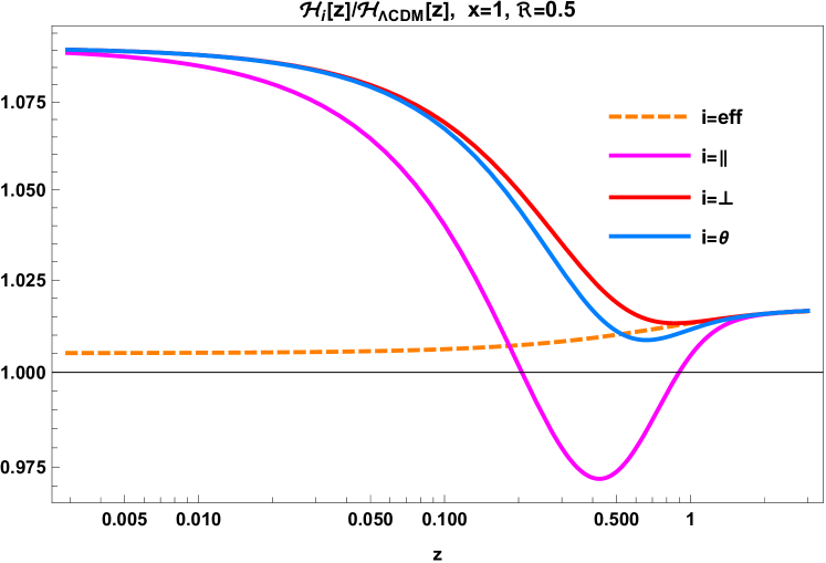
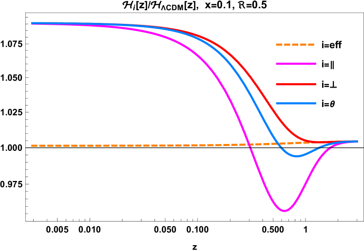
Figure 1: Here the $z$ evolution of the ratios between the asymptotic value of ${\cal H}_{\perp}(z\gg 1)$ of eq. (6.26) that we call ${\cal H}_{eff}$, the longitudinal ${\cal H}_{\parallel}(z)$ of eq. (2.20), the transverse ${\cal H}_{\perp}(z)$ of eq. (2.14) and the local ${\cal H}_{\theta}(z)$ of eq. (2.21) over the ${\cal H}_{\Lambda CDM}(z)$ of (6.4), for fixed $\Re=0.5$ with $x=1$ (only DE) to the left and $x=0.1$ (mainly DM) to the right.

To probe the matching with the FRW early-time dynamics [17], we need to expand our formulas in the large $z$ limit. In the asymptotic limit $z\gg 1$ (i.e. $a_{0}(z)\to 0$), we find that $r_{0}(z)$ approaches a finite value, which corresponds to the event horizon of the FRW model, $r_{0}(z)\to r_{H}\equiv\frac{2\,}{H_{0}\,\sqrt{\Omega_{m}}}\;_{2}F_{1}\left(\frac{1}{6},\frac{1}{2};\frac{7}{6};-\frac{\Omega_{\Lambda}}{\Omega_{m}}\right)\sim\frac{3.3}{H_{0}}$. For the transverse expansion rate (2.14) we can then express the asymptotic expansion in terms of the improved effective densities

$${\cal H}_{eff}(z)^{2}\equiv{\cal H}_{\perp}^{2}(z\gg 1) \simeq H_{0}^{2}\left(\frac{\Omega^{eff}_{m}}{a_{0}(z)^{3}}+\frac{\Omega^{eff}_{\kappa,\perp}}{a_{0}(z)^{2}}+\Omega^{eff}_{\Lambda}\right)+{\cal O}(a_{0}(z))$$ (6.26)

$$\hskip-113.81102pt\Omega^{eff}_{m}=\Omega_{m}\,\left(1-3\,\frac{a_{1}(z)}{a_{0}(z)}\right)_{z\gg 1},\quad\Omega^{eff}_{\kappa,\perp}=\frac{2}{5}\,\frac{\,{\bf e}_{1}(r_{H})}{r_{H}^{2}\,H_{0}^{2}},\quad\Omega^{eff}_{\Lambda}=\Omega_{\Lambda}$$

where the ratio $\left(\frac{a_{1}(z)}{a_{0}(z)}\right)_{z\gg 1}$ in obtained integrating eq. (6.13) and it results a finite number. Note that for the other Hubble rates (2.20, 2.21), we found some differences

$${\cal H}_{\parallel}^{2}\sim H_{0}^{2}\left(\frac{\Omega^{eff}_{m}}{a_{0}(z)^{3}}+\frac{\Omega^{eff}_{\kappa,\parallel}}{a_{0}(z)^{2}}+\Omega^{eff}_{\Lambda}\right)+{\cal O}(a_{0}(z))$$

$${\cal H}_{\theta}^{2}\sim H_{0}^{2}\left(\frac{\Omega^{eff}_{m}}{a_{0}(z)^{3}}+\frac{\Omega^{eff}_{\kappa,\theta}}{a_{0}(z)^{2}}+\Omega^{eff}_{\Lambda}\right)+{\cal O}(a_{0}(z))$$

$$\Omega^{eff}_{\kappa,\parallel}=\left(1-2\frac{r_{H}^{2}}{\Delta^{2}}\right)\,\Omega^{eff}_{\kappa,\perp},\qquad\Omega^{eff}_{\kappa,\theta}=\left(1-\frac{2}{3}\,\frac{r_{H}^{2}}{\Delta^{2}}\right)\,\Omega^{eff}_{\kappa,\perp}$$ (6.27)

where we see that while $\Omega^{eff}_{\kappa,\perp}$ is positive defined (6.23), $\Omega^{eff}_{\kappa,\parallel}$ and $\Omega^{eff}_{\kappa,\theta}$ are positive only for small ratios $\frac{r_{H}^{2}}{\Delta^{2}}\sim\frac{10}{\Re^{2}}$ i.e. for bubbles with $\Re\geq 0.07$ and $\Re\geq 0.04$. The $1\,\sigma$ constraints, from the combination of Planck, lensing and BAO data [2], for the spatial curvature and the matter density are given by

$$\Omega_{\kappa}=0.0007\pm 0.0019,\qquad\Omega_{m}=0.3081\pm 0.0065$$ (6.28)

In the fig.2, we apply the constraints on $\Omega^{eff}_{\kappa,i}$ and $\Omega^{eff}_{m}$, which determine the allowed $x-\Re$ parameter space at 1-2 $\sigma$ level. The strongest constraint, among the three components $\Omega^{eff}_{\kappa,i}$, comes from $\Omega^{eff}_{\kappa,\parallel}$ and at 1 $\sigma$ level, the left fig.2, is pushing for values of $\Re\sim 0.4-0.6$ for large $x$ or for small $x$ values (always $x\geq 0.06$) it is possible also $\Re\sim 2.3$. In any case the 2 $\sigma$ level bounds are much more approximate, see the right fig.2. This initial constraint on the parameter space arises from matching with the early-time cosmology. For the late time cosmological parameters , we present figures for various quantities: $w_{\parallel,\perp}(0)$ (see fig.3), the present-time deceleration parameter $Q_{0}$ (see fig.5 on the left), the jerk parameter $J_{0}$ (see fig.5 on the right), and finally, the first coefficient of the redshift drift $\frac{\dot{z}(0)}{z}$ (see fig.9).

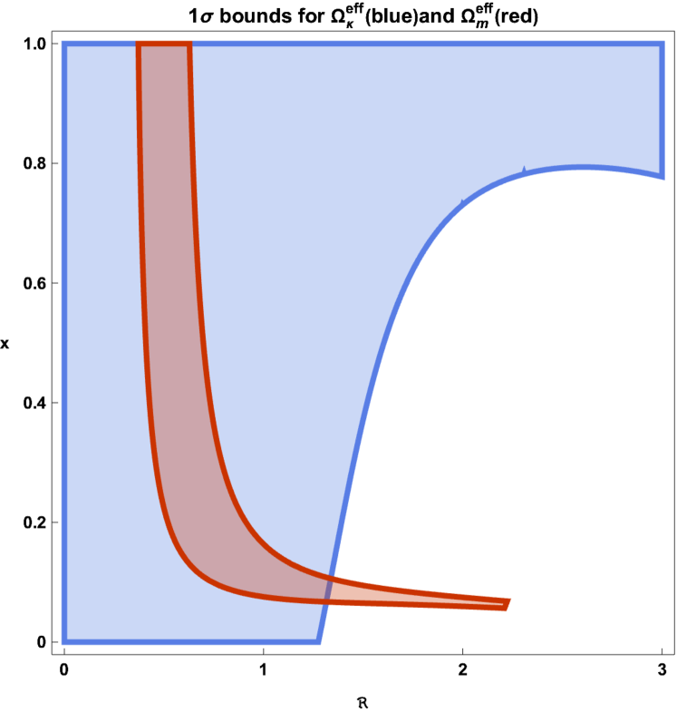
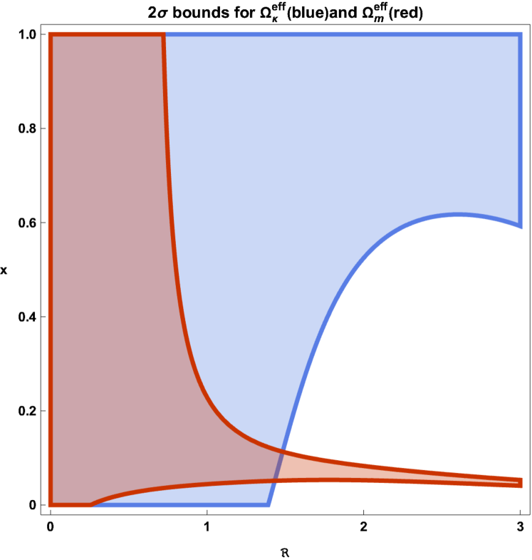
Figure 2: We implement in the parameter space $(x-\Re)$ the constraints (6.28) for $\Omega_{m}^{eff}$ (in red) and $\Omega_{\kappa,\parallel}^{eff}$ (in blue). On the left we have the $1\;\sigma$ bounds and on the right the $2\;\sigma$ bounds. The overlap of the two figures will be the parameter space that we consider in the rest of the paper.

6.2.1 Effective equation of state

An interesting function that characterises the $z$-derivative of the Hubble functions ${\cal H}(z)$ are the effective equation of state so defined

$$w_{i}(z)=-1+\frac{2}{3}\,\frac{d\,{\cal H}_{i}(z)}{d\,\log(1+z)},\qquad i=\parallel,\perp,\theta$$ (6.29)

Their general value at $z=0$ is given by

$$w_{\perp}(0) = -\Omega_{\Lambda}+\frac{2\,\Delta\mathcal{H}^{\prime}(0)}{3\,H_{0}^{2}}+\frac{\Delta H_{0}}{H_{0}}\,\left(\frac{10}{3\,(3\,\mathit{h}(1)-5)}+2\,\Omega_{\Lambda}\right)-\lambda(0)\,\Omega_{\Lambda}$$ (6.30)

$$w_{\parallel}(0) = w_{\perp}(0)+\frac{2\,\lambda(0)}{\Re^{2}}\,\left(1+\frac{20-14\,\mathit{h}(1)}{3\,(3\,\mathit{h}(1)-5)\,\Omega_{m}}\right)$$ (6.31)

once we choose the functional form (6.23, 6.24) we have ($w_{\Lambda CDM}(0)=-\Omega_{\Lambda}=-0.7$)

$$w_{\perp}(0)=w_{\Lambda CDM}(0)+\left(0.13+\frac{0.06\,x\,\Re^{2}}{0.25+x}\right),\qquad w_{\parallel}(0)\simeq w_{\perp}(0)-\frac{0.475\,x}{0.25+x}$$ (6.32)

that implies $\left.w_{\parallel}(0)\right|_{x=0}<w_{\perp}(0)<\left.w_{\parallel}(0)+0.38\right|_{x=1}$. Further the effective eqs of state have a minimum, one for $w^{min}_{\perp}(0)=-0.69$ when $\Re\to 0$ or $x\to 0$ and one for $w^{min}_{\parallel}(0)=-1.07$ when $x\to 1,\,\Re\to 0$ (note the fact that $w_{\parallel}$ can be less than -1 for a period [38]).

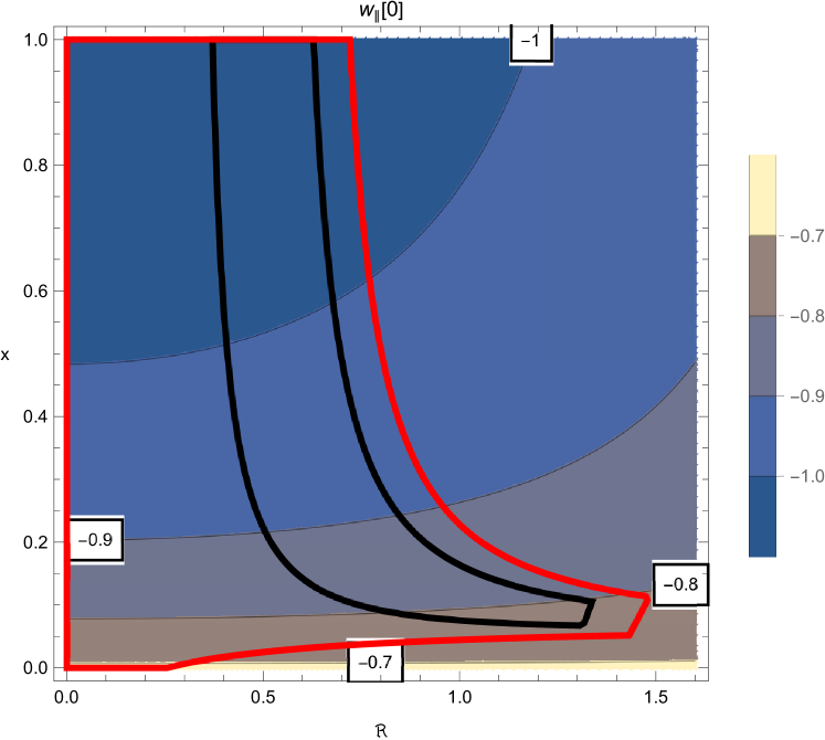
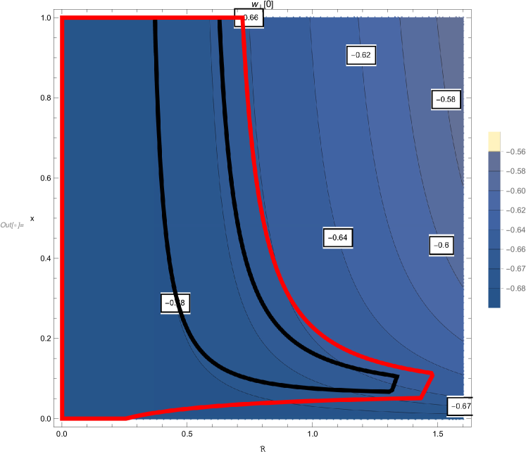
Figure 3: On the left, we show the contourplot of $w_{\parallel}(0)$ (6.31) and on the right, the contourplot of $w_{\perp}(0)$ (6.30). The black and red curves denote the $1-2\,\sigma$ regions from fig.2.

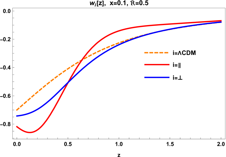
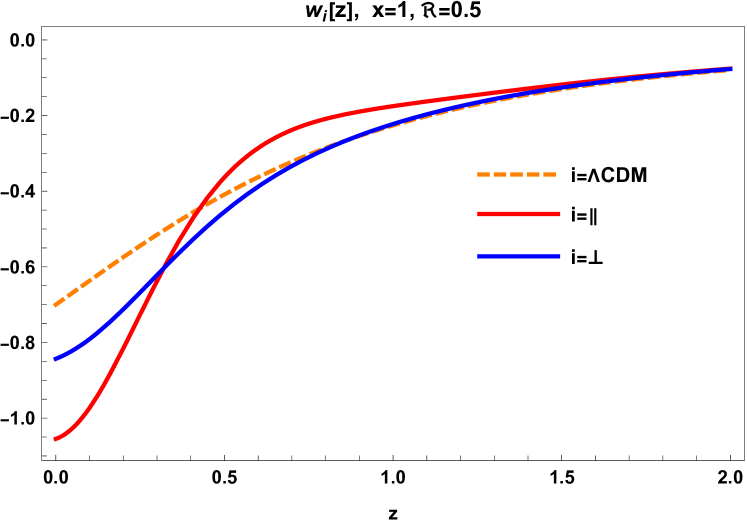
Figure 4: The $z$ evolution of various effective equation of states $w_{i}(z)$ (6.29): for $i=$$\Lambda$CDM , $i=\parallel$ longitudinal and $i=\perp$ transverse. On the left for $x=0.1,\,\Re=0.5$. On the right with $x=1,\,\Re=0.5$.

6.3 Deceleration and Jerk

Analogously to the effective eq. of state (6.29) we can define the deceleration and jerk $z-$ dependent parameters as

$$q_{i}(z)=-1+\frac{d\,{\cal H}_{i}}{d\log(1+z)},\quad i=\parallel,\,\perp,\,\theta$$ (6.33)

$$j_{i}(z)=(1+2\,q_{i})\,q_{i}+(1+z)\;\frac{dq_{i}}{dz}$$ (6.34)

and then (see also (5.15)) we can evaluate the deceleration $Q_{0}=q_{\parallel}(0)$ and the jerk parameter $J_{0}=j_{\parallel}(0)$ at present time to be (see (5.18) for the $\Lambda$CDM values)

$$Q_{0}=q_{\Lambda}+\left(-0.69+\frac{0.18+0.09\,x\,\Re^{2}}{x+0.25}\right)$$ (6.35)

$$J_{0}=j_{\Lambda}+\left(3.61-\frac{1.07}{x+0.25}-\frac{0.54}{\Re^{2}}\right)$$ (6.36)

where we see that for $Q_{0}$ we have a minimum $Q_{0}^{min}=-1.24$ for $\Re\to 0$ and $x\to 1$, while for $J_{0}$ we note the singularity $1/\Re^{2}$ that set strong bounds for small bubbles. In the literature the limits on such a parameters are strongly dependent from their $z$-functional form [39]. In ref [40] (where only supernovae in the redshift range $0.023\leq z\leq 0.15$ are used for the fit) it is reported the following limit $Q_{0}=-1.08\pm 0.29$ that, looking to fig.5, indicates a bubble dominated by a DE component with large $x$ values.

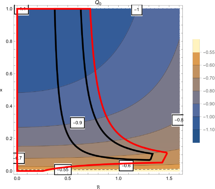
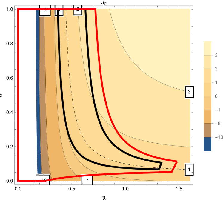
Figure 5: On the left we plot the value of the deceleration $Q_{0}$ (6.35). On the right, the value of the jerk $J_{0}$ (6.36). In black and red, the $1-2\,\sigma$ region of fig.2. The dashed lines are the corresponding $\Lambda$CDM values.

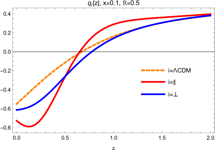
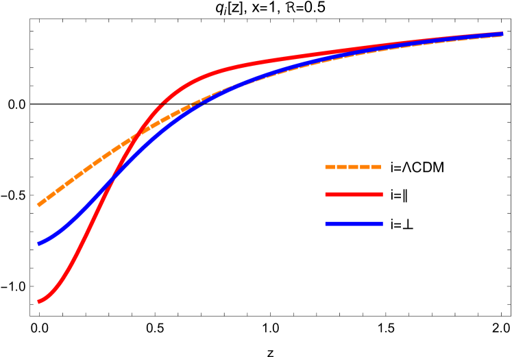
Figure 6: On the left the $z$ evolution of the decelerations $q_{i}(z)$ (6.33) for $\Lambda$CDM model, longitudinal and transverse when $x=0.1,\,\Re=0.5$. On the right the same but with $x=1,\,\Re=0.5$.

6.4 Drift

In order to characterise the $z$ dependence of the drift function $\dot{z}(z)$ (4) in the $x-\Re$ free parameter space we show various plots at different time scales.
First of all, we start from the nearby value $\dot{z}_{0}$ related to the expansion

$$\dot{z}(z)=\dot{z}_{0}\,z+{\cal O}(z^{2})$$ (6.37)

From fig.7 we see that, in the entire parameter space, we have systematically $\dot{z}_{0}>\dot{z}_{0}^{\Lambda CDM}=-q_{\Lambda}=0.55$ with a maximum of $\sim 0.83$ for large $x$ and small $\Re$.
To further characterise the $\dot{z}$ evolution we note two crucial features (see fig.9):

• A maximum around $z_{m}\sim 1$ that we denote as $\dot{z}^{max}$ (i.e. $\dot{z}^{max}=\dot{z}(z_{m})$).

• A zero point where $\dot{z}(z_{0})=0$, that happens near $z_{0}\sim 2$.

In particular for the $\Lambda$CDM model, we have $z^{\Lambda CDM}_{m}=0.94$ and $\dot{z}^{max}_{\Lambda CDM}/H_{0}=0.24$ and the zero point at $z^{\Lambda CDM}_{0}=2.09$. In fig.8 we contourplot the values of $\dot{z}^{max}/H_{0}$ (on the left) and the value of $z_{m}$ (on the right) as a function of $x-\Re$. We observe that $\dot{z}^{max}/H_{0}$ is slightly larger than in the $\Lambda$CDM model in the preferred region of parameter space, while in general, $z_{m}$ is smaller that the $\Lambda$CDM value. This implies that the maximum drift occurs earlier in our model. Finally, in fig.9, we show the $z$ evolution of the drift (4) for two representative values in the $x-\Re$ parameter space. In summary, we find in our model, the redshift drift starts with a steeper slope near the origin, reaches its maximum earlier than in the $\Lambda$CDM model, and attains a maximum value that is only slightly larger (at most 15 %) than the $\Lambda$CDM model. Afterward, the drift returns to zero earlier than in the $\Lambda$CDM model.

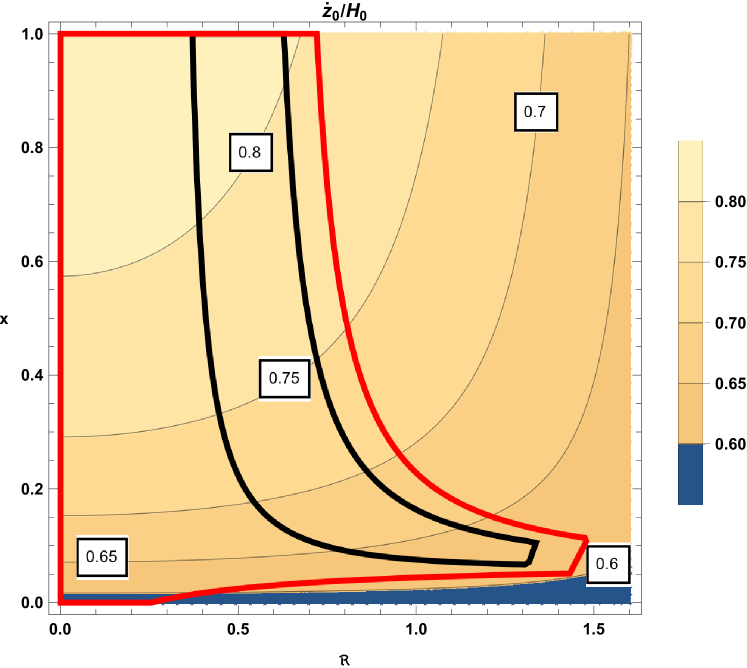
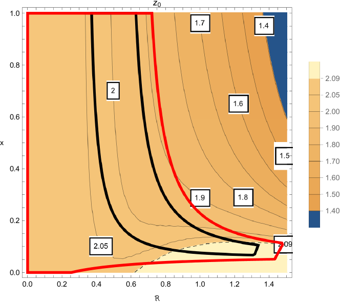
Figure 7: On the left, we show the contourplot $\dot{z}_{0}/H_{0}$ (6.37). On the right, we present the contourplot of the zero point $z_{0}$, where $\dot{z}(z_{0})=0$. For the $\Lambda$CDM model, we have $\dot{z}_{0}/H_{0}=-q_{0}=0.55$ and $z^{\Lambda CDM}_{0}=2.089$. The black and red curves denote the $1-2\,\sigma$ regions from fig.2.

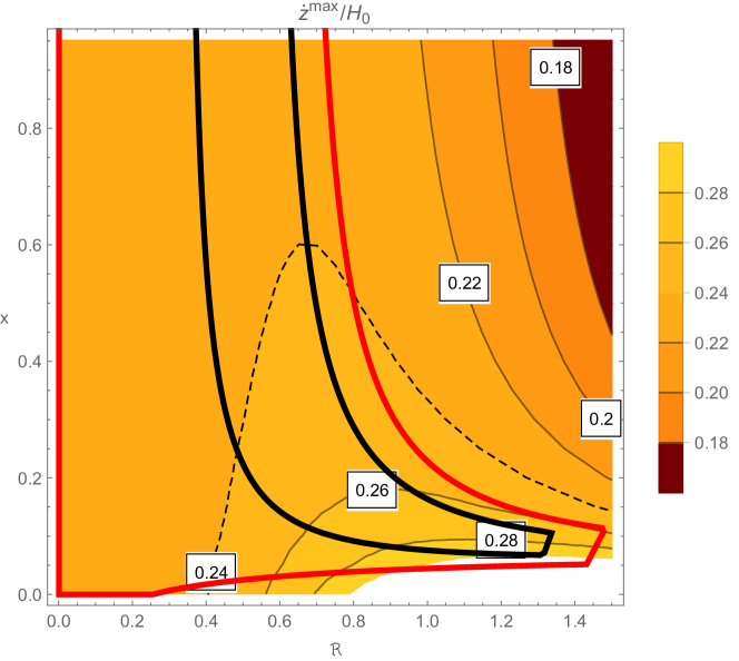
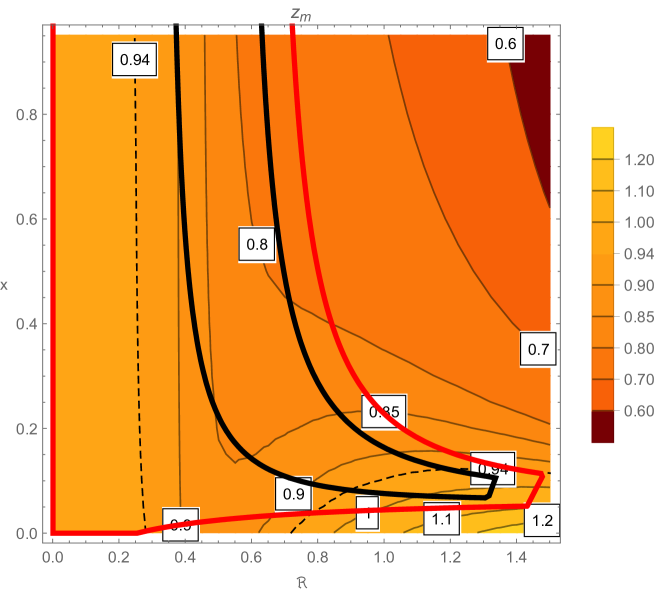
Figure 8: On the left, we show the contourplot of the maximum $\dot{z}^{max}$ , which occurs at $z_{m}$. On the right, we present the contourplot of $z_{m}$, where $\dot{z}(z_{m})=\dot{z}^{max}$. For the $\Lambda$CDM model, we find $z_{m}=0.94$ and $\dot{z}^{max}/H_{0}=0.24$. The black and red curves denote the $1-2\,\sigma$ regions from fig.2.

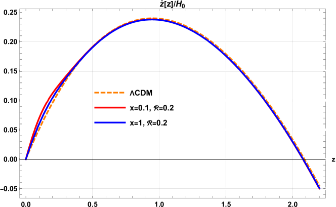
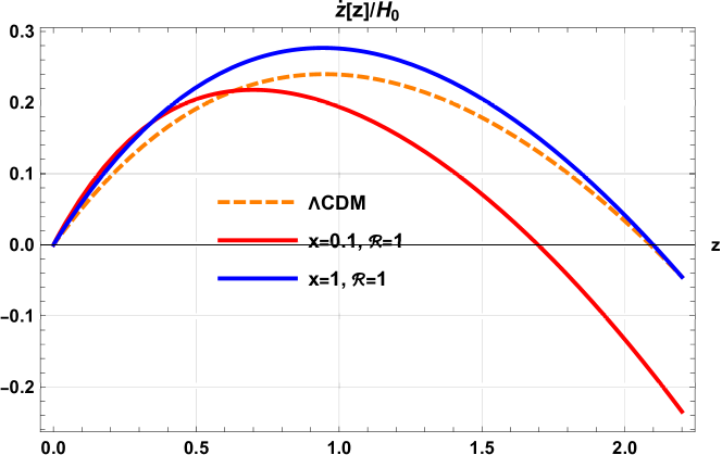
Figure 9: The redshift evolution of $\dot{z}(z)/H_{0}$ is shown for the $\Lambda$CDM model (4.10) and our model (4). On the left, we plot the results for $x=0.1$ and $x=1$ with a small value of $\Re=0.2$. On the right, we show the same values of $x$ for a larger value of $\Re=1$.

7 Conclusions

We analysed the dynamics of a cosmological model with a Locally Rotationally Symmetric spacetime coupled with a specific perfect fluid. The key feature of this fluid is the presence of a space-dependent CC and, simultaneously, a DM component, both exhibiting the same exponential suppressing profile for the inhomogeneities (6.23). A theoretical study of such a fluid is presented in [6], where only the space-dependent CC component was considered. Here, we skip the detailed theoretical aspects and instead postulate a perfect fluid EMT (2.7), where the energy density and pressure contains both DM and DE component (2.6). Using a Lema$\hat{\rm i}$tre metric in comoving coordinates, we show that the Einstein eqs (2.17, 2.14, 2.19) are solvable, modulo some space-dependent functions that arise from boundary conditions. A peculiarity of such a models, where the homogeneity of the spacetime is broken, is the presence of multiple independent expansion rates: the longitudinal ${\cal H}_{\parallel}$ (2.20), the transverse ${\cal H}_{\perp}$ (2.14), and the volume expansion rate ${\cal H}_{\theta}$ (2.21). In a FRW universe, these rates collapse into a single function, whereas in a LTB spacetime, only two of them remain independent (2.26).
In Chapter 3, we derive the null geodesic eqs and the variation of the redshift $z$ along the light path (3.11). In Chapter 4, we present the explicit eqs for the redshift drift, extended to the Lema$\hat{i}$tre metric (4). In Chapters 5 and 6, we solve both the Einstein evolution eqs and the light geodesic paths in two different approximation schemes.
In Chapter 5, we use a space Taylor expansion around the center and compute, order by order, various cosmographic observables, such as the decelaration parameter $Q_{0}$ (5.20) and the jerk $J_{0}$ (5.20). In eq.(5.28), we provide the leading ${\cal O}(z)$ correction to the redshift drift (the second order ${\cal O}(z^{2})$ corrections are presented in Appendix B). We establish a consistency relationship between the leading ${\cal O}(z)$ corrections to the Hubble rates and the redshift drift (5.30).
In Chapter 6, we expand around FRW solution and treat all terms that break homogeneity as perturbations (see (6.2)). The perturbed metric is derived from eqs (6.5, 6.6, 6.7). The solutions to the null geodesic eqs are provided in Chapter 6.1 (6.12, 6.13, 6.14). This allows us to match the model with the FRW external space, where the initial densities $\Omega_{i}$ get renormalised at large distances to $\Omega_{i}^{eff}$ (6.26). We impose the Planck constraints [2] on $\Omega_{i}^{eff}$ to obtain bounds on the parameters space, specifically for $x$, the fraction of DM versus DE (6.21), and the size of the bubble $\Re$ (6.23, 6.24). These bounds are illustrated in fig.2. Notably, we find, at 1-$\sigma$ level, an absolute bound of $x\gtrsim 0.07$ and also $\Re\lesssim 1.3$, further for $x\gtrsim 0.3$ the range of $\Re$ is getting narrowed: $0.4\lesssim\Re\lesssim 0.6$. So a pure DM profile with $x=0$ will be excluded at this level. At 2-$\sigma$ level, the above bounds get relaxed however an upper bound of $\Re\lesssim 0.78$ for a DE dominated bubble (large $x\gtrsim 0.3$ values) remains. A small bubble of DM with $x=0$ is allowed for $\Re\lesssim 0.25$. In fig.1, we show the evolution of the various Hubble parameters with redshift for both large and small $x$ values at fixed $\Re=0.5$.
To extract more physical insights, we study the evolution of the effective equation of state as a function of $z$ for different Hubble functions (6.29). At the origin ($z\to 0$), the effective eq.of state along the light of sight $w_{\parallel}(0)$ is always smaller that the transverse one $w_{\perp}(0)$ with minimum values of $w_{\parallel}(0)^{Min}\sim-1.07$ and $w_{\perp}(0)^{Min}\sim-0.69$. During the $z$ evolution (see fig.4), we observe a crossing where $w_{\parallel}(z)$ becomes larger than $w_{\parallel}(z)$ followed by a gradual approach to the $\Lambda$CDM equation of state, $w_{\Lambda CDM}(z)$.
For the cosmographic deceleration parameter $Q_{0}$ and jerk $J_{0}$, we find a minimum of $Q^{min}_{0}=-1.24$, to be compared with $-0.55$ in the $\Lambda$CDM, and a maximum of $J_{0}^{max}=3.75$ (for very large $\Re$ values and $x\to 1$), compared with 1, with no lower bound for negative $J_{0}$ values. For the $z$ evolution of the $q_{i}(z)$ functions, we find $q_{\parallel}(z)<q_{\perp}(z)$ for small $z$ ($z<\Re$), and around $z\sim\Re$, $q_{\parallel}(z)>q_{\perp}(z)$, eventually merging asymptotically with $q_{\Lambda CDM}(z)$.
For the drift, we compute the nearby values, i.e., the leading term $\dot{z}_{0}$ (where $\dot{z}\sim\dot{z}_{0}\,z+{\cal O}(z^{2})$) as a function of the free parameters $x-\Re$, as shown in the left panel of fig.7. The typical shape of the $\dot{z}(z)$ curve resembles a parabola, crossing the origin (see fig.9). The ”vertex” corresponds to the maximum of this function, which occurs at $z_{m}$, where $\dot{z}(z_{m})=\dot{z}^{max}$. Another interesting point is the $z_{0}$ coordinate of the second null point, where $\dot{z}(z_{0})=0$. All the values of $\dot{z}^{max}$, $z_{m}$ and $z_{0}$ are functions of the $x-\Re$ parameters, which we plot in fig.7 and fig.8.
In summary, we studied some of the main features of this exotic model, which, if the $H_{0}$ crisis is confirmed, could provide valuable insights. The choice of a single exponential behaviour for the perturbations (6.23) is motivated by the economy of the free parameters ($x$ for weighing DM versus DE, and $\Delta$ or $\Re$ for the size of the bubble). Note that the full amplitude of the effect (DE+DM) is fixed by the observed $\Delta H_{0}$ (see eq. (6.22)). Ultimately, a functional analysis that accommodates all present observables would provide full flexibility due to the arbitrariness of space-dependent functions.

Appendix A 1+3 and 1+1+2 Formalism

For review/applications of the 1+3 and the 1+1+2 formalism see [41] and [42].

• 1+3 Formalism
  The spacetime is split into time and space relative to a fundamental observer, represented by the timelike unit vector field $u^{\alpha}$, which corresponds to the observer’s 4-velocity. In this framework, the 1+3 covariant threading irreducibly decomposes any 4-vector into a scalar part parallel to $u^{\alpha}$ and a 3-vector part orthogonal to $u^{\alpha}$. Furthermore, any second rank tensor is covariantly and irreducibly split into scalar, 3-vector and projected symmetric trace-free 3-tensor components. The projection tensor onto the metric of the 3-space (S) orthogonal to $u^{\alpha}$ is given by

  $$h_{\alpha\beta}=g_{\alpha\beta}+u_{\alpha}\;u_{\beta},\qquad h^{\alpha}_{\alpha}=3$$ (A.1)

  The covariant derivative of a scalar function $f$ projected along $u^{\alpha}$ is so defined

  $$\dot{f}=u^{\alpha}\nabla_{\alpha}f$$ (A.2)

  We can decompose the covariant derivative of $u^{\alpha}$ orthogonal to $u^{\alpha}$ giving

  $$\nabla_{\alpha}\;u_{\beta}=-u_{\alpha}\;{\cal A}_{\beta}+\frac{1}{3}\;\theta\;h_{\alpha\beta}+\sigma_{\alpha\beta}+\omega_{\beta\alpha}$$ (A.3)

  where we defined the following structures

  • 4-Acceleration

    $${\cal A}_{\alpha}\equiv u^{\beta}\nabla_{\beta}\;u_{\alpha}\equiv\dot{u}_{\alpha}$$ (A.4)

  • Expansion

    $$\theta\equiv\nabla^{\alpha}\;u_{\alpha}$$ (A.5)

  • Shear

    $$\sigma_{\alpha\beta}=h^{\lambda}_{\beta}\;\nabla_{(\lambda}\;u_{\rho)}\;h_{\alpha}^{\rho}-\frac{1}{3}\;\theta\;h_{\alpha\beta}$$ (A.6)

  • Vorticity

    $$\omega_{\alpha\beta}=h^{\lambda}_{\beta}\;\nabla_{[\lambda}\;u_{\rho]}\;h_{\alpha}^{\rho},\qquad\omega^{\alpha}=\epsilon^{\alpha\beta\gamma}\;\omega_{\beta\gamma}$$ (A.7)

• 1+1+2 Formalism
  The 1 + 1 + 2 approach is based on a double foliation of the spacetime. Projection tensor which represents the metric of the 2-spaces orthogonal to $u^{\alpha}$ and a spacelike ($v^{\alpha}\;v_{\alpha}=1$) vector $v^{\alpha}$.

  $$N_{\alpha\beta}=h_{\alpha\beta}-v_{\alpha}\;v_{\beta},\qquad N^{\alpha}_{\alpha}=2$$ (A.8)

  The hat-derivative is the derivative along the vector field $v^{\alpha}$ in the surfaces orthogonal to $u^{\alpha}$, for a scalar function $f$ we have the definitions

  $$\hat{f}=v^{\alpha}\nabla_{\alpha}f$$ (A.9)

  We are now able to decompose the covariant derivative of $v^{\alpha}$ orthogonal to $u^{\alpha}$ giving

  $$\nabla_{\alpha}\;u_{\beta}=-{\cal A}\;u_{\alpha}\;e_{\beta}+\left(\frac{\theta}{3}+\Sigma\right)\;v_{\alpha}\;v_{\beta}+\left(\frac{\theta}{3}-\frac{\Sigma}{2}\right)\;N_{\alpha\beta}+\Omega\;\epsilon_{\alpha\beta}$$ (A.10)

  $$\nabla_{\alpha}\;v_{\beta}=-{\cal A}\;u_{\alpha}\;u_{\beta}+\left(\frac{\theta}{3}+\Sigma\right)\;v_{\alpha}\;u_{\beta}+\frac{\phi}{2}\;N_{\alpha\beta}+\xi\;\epsilon_{\alpha\beta}$$ (A.11)

  $$D_{\alpha}\;v_{\beta}=v_{\beta}\;a_{\beta}+\frac{1}{2}\;\phi\;N_{\alpha\beta}+\xi\;\epsilon_{\alpha\beta}+\zeta_{\alpha\beta}$$ (A.12)

  where

  • Sheet expansion

    $$\phi=\delta_{\alpha}\;v^{\alpha}=D_{\alpha}\;v^{\alpha}$$ (A.13)

  • Twisting of the sheet (the rotation of $v^{\alpha}$)

    $$\xi=\frac{1}{2}\epsilon^{\alpha\beta}\;\delta_{\alpha}v_{\beta}$$ (A.14)

  • Acceleration of $v^{\alpha}$

    $$a_{\alpha}=\hat{v}_{\alpha}$$ (A.15)

  • Shear of $v^{\alpha}$

    $$\zeta_{\alpha\beta}=\delta_{\{\alpha}\;v_{\beta\}}$$ (A.16)

  Note the following identities and definitions

  $$v\cdot u=0,\quad v^{2}=1,\quad v\cdot a=-u\cdot\dot{v},\quad v\cdot\dot{v}=0$$ (A.17)

  $${\cal A}={\cal A}^{\alpha}v_{\alpha}=-u^{\alpha}\;\dot{v}_{\alpha},\quad\Sigma=v^{\alpha}\sigma_{\alpha\beta}v^{\beta},\quad\Omega=v^{\alpha}\omega_{\alpha\beta}v^{\beta},\quad$$ (A.18)

Appendix B Small $z$ expansion for the redshift drift

Starting from eq.(4) we factorise the two contributions (the first is local $\dot{z}_{L}(z)$, the second is non local $\dot{z}_{NL}(z)$ in the $z$ space)

$$\dot{z}(z)=\underbrace{H_{0}(1+z)-{\cal H}_{\parallel}(z)}_{\equiv\,\dot{z}_{L}(z)}+\underbrace{(1+z)\int^{z}_{0}\frac{1}{(1+z^{\prime})^{2}}\frac{\partial_{r}\log(F\,{\cal H}_{\parallel})}{X}\,dz^{\prime}}_{\equiv\,\dot{z}_{NL}(z)}$$ (B.1)

While it is straightforward the small $z$ expansion of the local contribution, for $\dot{z}_{1}(z)$ we can use the following formula

$$(1+z)\,\int^{z}_{0}dz^{\prime}\,f(z^{\prime})\simeq f(0)\,z+\left(f(0)+\frac{f^{\prime}(0)}{2}\right)\,z^{2}+{\cal O}(z^{3})$$ (B.2)

The leading order ${\cal O}(z)$ corrections are given by

$$\dot{z}_{L}(z)=z\,H\,\left(1-\frac{3\,\Omega_{m}}{2}-\Omega_{\kappa}+2\,\Omega_{\chi}-R_{2}^{\prime}(1)\right)+{\cal O}(z^{2}),\;\;$$

$$\dot{z}_{NL}(z)\to z\,H\,\left(-\frac{3\,\Omega_{\chi}}{2}+R_{2}^{\prime}(1)\right)+{\cal O}(z^{2}),$$

$$\dot{z}(z)=Hz\left(1-\frac{3\,\Omega_{m}}{2}-\Omega_{\kappa}+\frac{\Omega_{\chi}}{2}\right)+{\cal O}(z^{2})$$ (B.4)

The corrections from $\dot{z}_{L}(z)$ and $\dot{z}_{NL}(z)$ are of the same order as noted in [25], [33].

References

- [1] S. Perlmutter et al. [Supernova Cosmology Project], Measurements of and from 42 High Redshift Supernovae, Astrophys. J. 517 (1999), 565-586, doi:10.1086/307221, [arXiv:astro-ph/9812133 [astro-ph]].
- [2] N. Aghanim et al. [Planck], Planck 2018 results. VI. Cosmological parameters, Astron. Astrophys. 641 (2020), A6, [erratum: Astron. Astrophys. 652 (2021), C4], doi:10.1051/0004-6361/201833910, [arXiv:1807.06209 [astro-ph.CO]].
- [3] A. G. Riess, W. Yuan, L. M. Macri, D. Scolnic, D. Brout, S. Casertano, D. O. Jones, Y. Murakami, L. Breuval and T. G. Brink, et al. A Comprehensive Measurement of the Local Value of the Hubble Constant with 1 km/s/Mpc Uncertainty from the Hubble Space Telescope and the SH0ES Team, Astrophys. J. Lett. 934 (2022) no.1, L7, doi:10.3847/2041-8213/ac5c5b, [arXiv:2112.04510 [astro-ph.CO]].
- [4] E. Di Valentino, O. Mena, S. Pan, L. Visinelli, W. Yang, A. Melchiorri, D. F. Mota, A. G. Riess and J. Silk, In the realm of the Hubble tension—a review of solutions,” Class. Quant. Grav. 38 (2021) no.15, 153001, doi:10.1088/1361-6382/ac086d, [arXiv:2103.01183 [astro-ph.CO]].
- [5] J. P. Hu and F. Y. Wang, Hubble Tension: The Evidence of New Physics, Universe 9 (2023) no.2, 94, doi:10.3390/universe9020094, [arXiv:2302.05709 [astro-ph.CO]].
- [6] D. Comelli, A space dependent Cosmological Constant, JCAP 04 (2024), 080, doi:10.1088/1475-7516/2024/04/080, [arXiv:2311.15866 [gr-qc]].
- [7] G. Ballesteros, D. Comelli and L. Pilo, Thermodynamics of perfect fluids from scalar field theory, Phys. Rev. D 94 (2016) no.2, 025034, doi:10.1103/PhysRevD.94.025034, [arXiv:1605.05304 [hep-th]]. M. Celoria, D. Comelli and L. Pilo, Intrinsic Entropy Perturbations from the Dark Sector, JCAP 1803 (2018) no.03, 027, doi:10.1088/1475-7516/2018/03/027, [arXiv:1711.01961 [gr-qc]].
- [8] P. K. Aluri, P. Cea, P. Chingangbam, M. C. Chu, R. G. Clowes, D. Hutsemékers, J. P. Kochappan, A. M. Lopez, L. Liu and N. C. M. Martens, et al. Is the observable Universe consistent with the cosmological principle?, Class. Quant. Grav. 40 (2023) no.9, 094001, doi:10.1088/1361-6382/acbefc, [arXiv:2207.05765 [astro-ph.CO]].
-
[9]
G. F. R. Ellis,
Dynamics of pressure free matter in general relativity,
J. Math. Phys. 8 (1967) 1171,
doi:10.1063/1.1705331.
J. M. Stewart and G. F. R. Ellis, Solutions of Einstein’s equations for a fluid which exhibit local rotational symmetry, J. Math. Phys. 9 (1968) 1072, doi:10.1063/1.1664679.
H. van Elst and G. F. R. Ellis, The Covariant approach to LRS perfect fluid space-time geometries, Class. Quant. Grav. 13 (1996) 1099, [gr-qc/9510044]. - [10] K. Enqvist, Lemaitre-Tolman-Bondi model and accelerating expansion, Gen. Rel. Grav. 40 (2008), 451-466, doi:10.1007/s10714-007-0553-9, [arXiv:0709.2044 [astro-ph]]. K. Enqvist and T. Mattsson, The effect of inhomogeneous expansion on the supernova observations, JCAP 02 (2007), 019, doi:10.1088/1475-7516/2007/02/019, [arXiv:astro-ph/0609120 [astro-ph]].
- [11] J. Garcia-Bellido and T. Haugboelle, Confronting Lemaitre-Tolman-Bondi models with Observational Cosmology, JCAP 04 (2008), 003, doi:10.1088/1475-7516/2008/04/003, [arXiv:0802.1523 [astro-ph]].
- [12] K. Bolejko and P. Lasky, Pressure gradients, shell crossing singularities and acoustic oscillations - application to inhomogeneous cosmological models, Mon. Not. Roy. Astron. Soc. 391 (2008), 59, doi:10.1111/j.1745-3933.2008.00555.x, [arXiv:0809.0334 [astro-ph]]
- [13] R. Moradi, J. T. Firouzjaee and R. Mansouri, The spherical perfect fluid collapse with pressure in the cosmological background, doi:10.1142/9789813226609_0593, [arXiv:1301.1480 [gr-qc]].
- [14] A. A. H. Alfedeel and C. Hellaby, The Lemaitre Model and the Generalisation of the Cosmic Mass, Gen. Rel. Grav. 42 (2010), 1935-1952, doi:10.1007/s10714-010-0971-y, [arXiv:0906.2343 [gr-qc]].
- [15] H. Alnes and M. Amarzguioui, CMB anisotropies seen by an off-center observer in a spherically symmetric inhomogeneous Universe, Phys. Rev. D 74 (2006), 103520, doi:10.1103/PhysRevD.74.103520, [arXiv:astro-ph/0607334 [astro-ph]].
- [16] G. Cusin, C. Pitrou and J. P. Uzan, Are we living near the center of a local void?, JCAP 03 (2017), 038, doi:10.1088/1475-7516/2017/03/038, [arXiv:1609.02061 [astro-ph.CO]].
- [17] T. Biswas, A. Notari and W. Valkenburg, Testing the Void against Cosmological data: fitting CMB, BAO, SN and H0, JCAP 11 (2010), 030, doi:10.1088/1475-7516/2010/11/030, [arXiv:1007.3065 [astro-ph.CO]].
- [18] G. Lematre, The expanding universe, Gen. Rel. Grav. 29 (1997) 641, [Annales Soc. Sci. Bruxelles A 53 (1933) 51], doi:10.1023/A:1018855621348.
- [19] C.Hellaby, Some Properties of Singularities in the Tolman Model, Ph.D.thesis, Queen’s University at Kinston, Ontario, 1985.
- [20] P. D. Lasky and K. Bolejko, The effect of pressure gradients on luminosity distance - redshift relations, Class. Quant. Grav. 27 (2010) 035011, doi:10.1088/0264-9381/27/3/035011, [arXiv:1001.1159 [astro-ph.CO]].
- [21] R. Jimenez, R. Maartens, A. R. Khalifeh, R. R. Caldwell, A. F. Heavens and L. Verde, Measuring the Homogeneity of the Universe Using Polarization Drift, JCAP 05 (2019), 048, doi:10.1088/1475-7516/2019/05/048, [arXiv:1902.11298 [astro-ph.CO]].
- [22] Synge,J.L.,Schild,A.:Tensor Calculus. University of Toronto, Toronto(1952). Synge, J.L.: Relativity: The General Theory. Series in Physics. North-Holland Pub. Co., Amsterdam (1960)
- [23] B. de Swardt, P. K. S. Dunsby and C. Clarkson, Gravitational Lensing in Spherically Symmetric Spacetimes, [arXiv:1002.2041 [gr-qc]].
- [24] O. Umeh, C. Clarkson and R. Maartens, Nonlinear relativistic corrections to cosmological distances, redshift and gravitational lensing magnification. II - Derivation, Class. Quant. Grav. 31 (2014), 205001, doi:10.1088/0264-9381/31/20/205001, [arXiv:1402.1933 [astro-ph.CO]].
- [25] S. M. Koksbang and A. Heinesen, Redshift drift in a universe with structure: Lemaître-Tolman-Bondi structures with arbitrary angle of entry of light, Phys. Rev. D 106 (2022) no.4, 043501, doi:10.1103/PhysRevD.106.043501, [arXiv:2205.11907 [astro-ph.CO]].
- [26] A. Sandage, The Change of Redshift and Apparent Luminosity of Galaxies due to the Deceleration of Selected Expanding Universes. Astrophys.J. 136 (1962) 319, doi = 10.1086/147385. G.C. McVittie, Appendix to The Change of Redshift and Apparent Luminosity of Galaxies due to the Deceleration of Selected Expanding Universes. Astrophys.J. 136 (1962) 334.
- [27] A. Loeb, Direct Measurement of Cosmological Parameters from the Cosmic Deceleration of Extragalactic Objects, Astrophys. J. Lett. 499 (1998), L111-L114, doi:10.1086/311375, [arXiv:astro-ph/9802122 [astro-ph]].
- [28] A. Heinesen, Redshift drift cosmography for model-independent cosmological inference, Phys. Rev. D 104 (2021) no.12, 123527, doi:10.1103/PhysRevD.104.123527, [arXiv:2107.08674 [astro-ph.CO]]. A. Heinesen, Multipole decomposition of redshift drift – model independent mapping of the expansion history of the Universe, Phys. Rev. D 103 (2021) no.2, 023537, doi:10.1103/PhysRevD.103.023537, [arXiv:2011.10048 [gr-qc]]. A. Heinesen and M. Korzyński, Exploring the rich geometrical information in cosmic drift signals with covariant cosmography, [arXiv:2406.06167 [astro-ph.CO]].
- [29] F. S. N. Lobo, J. P. Mimoso, J. Santiago and M. Visser, Dynamical Analysis of the Redshift Drift in FLRW Universes, Universe 10 (2024) no.4, 162, doi:10.3390/universe10040162, [arXiv:2210.13946 [gr-qc]].
- [30] C. M. Yoo, T. Kai and K. I. Nakao, Redshift drift in LTB universes, Phys.Rev.D83:043527,2011, doi:10.1103/PhysRevD.83.043527, [arXiv:1010.0091 [astro-ph.CO]].
- [31] P. Mishra and M. N. Célérier, Redshift and redshift drift in quasispherical Szekeres cosmological models and the effect of averaging, Phys. Rev. D 105 (2022) no.6, 063520, doi:10.1103/PhysRevD.105.063520, [arXiv:1403.5229 [astro-ph.CO]].
- [32] E. G. Chirinos Isidro, C. Zuñiga Vargas and W. Zimdahl, Simple inhomogeneous cosmological (toy) models, JCAP 05 (2016), 003, doi:10.1088/1475-7516/2016/05/003, [arXiv:1602.08583 [gr-qc]].
- [33] R. Codur and C. Marinoni, Redshift drift in radially inhomogeneous Lemaître-Tolman-Bondi spacetimes, Phys. Rev. D 104 (2021) no.12, 123531, doi:10.1103/PhysRevD.104.123531, [arXiv:2107.04868 [gr-qc]].
- [34] M. H. Partovi and B. Mashhoon, Toward Verification of Large Scale Homogeneity in Cosmology, Astrophys. J. 276 (1984) 4, doi:10.1086/161588.
- [35] J. Adamek, C. Clarkson, R. Durrer, A. Heinesen, M. Kunz and H. J. Macpherson, Towards Cosmography of the Local Universe, Open J. Astrophys. 7 (2024), 001c.118782, doi:10.33232/001c.118782, [arXiv:2402.12165 [astro-ph.CO]].
- [36] M. N. Celerier, Do we really see a cosmological constant in the supernovae data?, Astron. Astrophys. 353 (2000), 63-71, [arXiv:astro-ph/9907206 [astro-ph]].
- [37] V. Marra and M. Paakkonen, Exact spherically-symmetric inhomogeneous model with n perfect fluids, JCAP 01 (2012), 025, doi:10.1088/1475-7516/2012/01/025, [arXiv:1105.6099 [gr-qc]].
- [38] S. M. Carroll, M. Hoffman and M. Trodden, Can the dark energy equation-of-state parameter w be less than -1 ?, Phys. Rev. D 68 (2003), 023509, doi:10.1103/PhysRevD.68.023509, [arXiv:astro-ph/0301273 [astro-ph]].
- [39] A. Al Mamon and K. Bamba, Eur. Phys. J. C 78 (2018) no.10, 862, doi:10.1140/epjc/s10052-018-6355-2, [arXiv:1805.02854 [gr-qc]].
- [40] D. Camarena and V. Marra, Local determination of the Hubble constant and the deceleration parameter, Phys. Rev. Res. 2 (2020) no.1, 013028, doi:10.1103/PhysRevResearch.2.013028, [arXiv:1906.11814 [astro-ph.CO]].
- [41] G. F. R. Ellis and H. van Elst, Cosmological models: Cargese lectures 1998, NATO Sci. Ser. C 541 (1999) 1, doi:10.1007/978-94-011-4455-, [gr-qc/9812046].
-
[42]
C. A. Clarkson and R. K. Barrett,
Covariant perturbations of Schwarzschild black holes,
Class. Quant. Grav. 20 (2003) 3855,
doi:10.1088/0264-9381/20/18/301,
[gr-qc/0209051].
G. Betschart and C. A. Clarkson, Scalar and electromagnetic perturbations on LRS class II space-times, Class. Quant. Grav. 21 (2004) 5587, doi:10.1088/0264-9381/21/23/018, [gr-qc/0404116].
C. Clarkson, A Covariant approach for perturbations of rotationally symmetric spacetimes, Phys. Rev. D 76 (2007) 104034, doi:10.1103/PhysRevD.76.104034, [arXiv:0708.1398 [gr-qc]].
S. Carloni and D. Vernieri, Covariant Tolman-Oppenheimer-Volkoff equations. I. The isotropic case, Phys. Rev. D 97 (2018) no.12, 124056, doi:10.1103/PhysRevD.97.124056, [arXiv:1709.02818 [gr-qc]].