Plus-pure thresholds of some cusp-like singularities
in mixed characteristic

Abstract.

Log-canonical and $F$-pure thresholds of pairs in equal characteristic admit an analog in the recent theory of singularities in mixed characteristic, which is known as the plus-pure threshold. In this paper we study plus-pure thresholds for singularities of the form $p^{a}+x^{b}\in{\bf{Z}}_{p}[\![x]\!]$, showing that in a number of cases this plus-pure threshold agrees with the $F$-pure threshold of the singularity $t^{a}+x^{b}\in{\bf F}_{p}[\![t,x]\!]$. We also discuss a few other sporadic examples.

1. Introduction

Let $X$ be a smooth algebraic variety over ${\bf C}$, let $x\in X$ be a closed point and $D=(f=0)$ be a prime divisor containing $x$. If $R\colonequals\widehat{\mathcal{O}_{X,x}}$ denotes the completion of the local ring at $x$, the log-canonical threshold $\operatorname{lct}(R,f)$ is the threshold in $t$ at which the pair $(X,tD)$ becomes not log canonical at $x$; in other words, it is the first jumping number of the multiplier ideal $\mathcal{J}(R,f^{t})$. This invariant has been used prominently in birational algebraic geometry and the minimal model program; see [Kol97, Laz04] for some applications.

Log canonical pairs are closely related to $F$-pure pairs in characteristic $p>0$ [HW02, MS11, BST13]. Inspired by this connection, Takagi and Watanabe defined the $F$-pure threshold $\operatorname{{fpt}}(R,f)$ as the threshold in $t$ at which $(R,f^{t})$ becomes not $F$-pure [TW04], cf. [MTW05, HMTW08]. When $R$ is regular, this is also the first jumping number of the test ideal $\tau(R,f^{t})$, a characteristic-$p$ analog of the multiplier ideal. Note that there has been a great deal of effort directed towards computing the $F$-pure thresholds of specific (classes of) polynomials [ST09, Her15, Her14, BS15, MSV14, HNnBWZ16, HT17, DSNnB18, Mül18, Pag18, KKP⁺22, SV23].

In recent years, building upon the theory of Scholze’s perfectoid algebras [Sch12] and the work of André, Bhatt, Gabber, Heitmann-Ma and others [And18, Bha18, And20, Gab18, HM18, Bha20], the development of a theory of singularities in mixed characteristic is now underway [MS18, MS21, DT21, MST⁺22, BMP⁺23a, Rob22, HLS24, Mur21, CLM⁺22, BMP⁺23b, BMP⁺24, RV24]. This theory provides an analog for the multiplier and test ideals. The first jumping number—known as the plus-pure threshold—therefore provides an analog of the log-canonical and $F$-pure thresholds. A succint definition is as follows: if $(R,\mathfrak{m})$ is a regular complete local domain of mixed characteristic, and $0\neq f\in R$ is an element, then the plus-pure threshold of $(R,f)$ is given by

$$\operatorname{+pt}(R,f)\colonequals\sup\{t\in{\bf Q}_{>0}\ |\ f^{t}:R\longrightarrow R^{+}\text{ splits }\},$$

where $R^{+}$ is the absolute integral closure of $R$ (see Section 2.1 for other characterizations).

Except for some toric-type singularities, see for instance [Rob22], essentially no examples of plus-pure thresholds have been calculated (although some upper and lower bounds were known, and sometimes they coincide, see below). This paper begins this exploration by computing the plus-pure thresholds of some cusp-like singularities $f\colonequals p^{a}+x^{b}\in{\bf{Z}}_{p}[\![x]\!]$, where ${\bf Z}_{p}$ is the ring of $p$-adic integers. Indeed, unlike characteristic $p>0$, one cannot simply use Frobenius and so the computations become much more subtle.

Before we discuss our work, we remark that something was known about the examples $f\colonequals p^{2}+x^{3}\in{\bf Z}_{p}[\![x]\!]$ and $f\colonequals p^{3}+x^{2}\in{\bf Z}_{p}[\![x]\!]$. On the one hand, by [BMP⁺23a, Proposition 4.17, Lemma 4.18] or [MS21, Theorem 6.21] and [Bha20], if the map ${\bf Z}_{p}[\![x]\!]\longrightarrow{\bf Z}_{p}[\![x]\!]^{+}$ given by $1\mapsto f^{t}$ were to split for some $t\in{\bf Q}_{>0}$, the pair $({\bf Z}_{p}[\![x]\!],f^{t})$ would be log-terminal, then a blowup computation shows that $t<5/6$ and therefore $\operatorname{+pt}({\bf Z}_{p}[\![x]\!],f)\leq 5/6$. On the other hand, the $F$-pure threshold of the related polynomial $f_{0}\colonequals y^{2}+x^{3}\in{\bf F}_{p}[\![y,x]\!]$ provides a lower bound for $\operatorname{+pt}({\bf Z}_{p}[\![x]\!],f)$; indeed, combining [MST⁺22, Example 7.10] with [Bha20], we see that $f^{t}:{\bf Z}_{p}[\![x]\!]\longrightarrow{\bf Z}_{p}[\![x]\!]^{+}$ splits whenever $({\bf F}_{p}[\![y,x]\!],f_{0}^{t})$ is $F$-regular. We conclude that

$$\operatorname{{fpt}}\big{(}{\bf F}_{p}[\![y,x]\!],f_{0}\big{)}\leq\operatorname{+pt}\big{(}{\bf Z}_{p}[\![x]\!],f\big{)}\leq\frac{5}{6},$$

and we recall that the lower bound $\operatorname{{fpt}}({\bf F}_{p}[\![y,x]\!],f_{0})$ is known to be as follows (see [MTW05, Example 4.3]):

$$\operatorname{{fpt}}\big{(}{\bf F}_{p}[\![y,x]\!],f_{0}\big{)}=\begin{cases}1/2\text{ if }p=2\\ 2/3\text{ if }p=3\\ (5p-1)/6p\text{ if }p\equiv 5\text{ mod }6\\ 5/6\text{ if }p\equiv 1\text{ mod }6.\end{cases}$$

In particular, it was known that $\operatorname{+pt}({\bf Z}_{p}[\![x]\!],f)=5/6$ when $p\equiv 1\text{ mod }6$.

As our first contribution, we show that analogous upper and lower bounds hold for any cusp-like polynomial $f=p^{a}+x^{b}\in{\bf{Z}}_{p}[\![x]\!]$; this is somewhat painfully verified in Section 2.2 by utilizing some of the main results of [MS21, MST⁺22, BMP⁺23a].

Our main goal is then to show that, in many cases, one has $\operatorname{+pt}(R,f)=\operatorname{{fpt}}(R_{0},f_{0})$; in other words, that one has equality on the lower bound. For example, we prove that this is the case for the polynomials $f=p^{2}+x^{3}$ and $f=p^{3}+x^{2}$ discussed above. Note that, by Section 2.2 as mentioned above, one has $\operatorname{+pt}(f)={1\over a}+{1\over b}$ whenever $\operatorname{{fpt}}(R_{0},f_{0})={1\over a}+{1\over b}$, and some of the remaining cases are handled by the theorem below.

Main Theorem (Section 3).

Fix a prime $p>0$, let $R\colonequals{\bf Z}_{p}\llbracket x\rrbracket$ be a power series ring in one variable over the $p$-adic integers, and let $R_{0}\colonequals{\bf F}_{p}\llbracket y,x\rrbracket$ be a power series ring in two variables over ${\bf F}_{p}$. Fix integers $a,b\geq 2$ and consider the polynomials $f\colonequals p^{a}+x^{b}\in R$ and $f_{0}\colonequals y^{a}+x^{b}\in R_{0}$.

Assume that $\operatorname{{fpt}}(R_{0},f_{0})\neq{1\over a}+{1\over b}$, and fix an integer $e\geq 1$ such that $p^{e}\operatorname{{fpt}}(R_{0},f_{0})\in{\bf Z}$. If we have

$$\operatorname{{fpt}}(R_{0},f_{0})\geq\frac{1}{a}+\frac{1}{b}-\frac{1}{ap^{e}},$$

then $\operatorname{+pt}(R,f)=\operatorname{{fpt}}(R_{0},f_{0})$.

Note that an algorithm for the computation of $\operatorname{{fpt}}(R_{0},f_{0})$ is provided in [Her14, Her15], cf. [ST09] (we briefly discuss this algorithm in Section 3). It follows from some of the references above that, unless one has $\operatorname{{fpt}}(R_{0},f_{0})={1\over a}+{1\over b}$, the denominator of $\operatorname{{fpt}}(R_{0},f_{0})$ is a power of $p$, and therefore one can always choose an $e\geq 1$ as in the statement of the theorem.

Since the $F$-pure threshold $\operatorname{{fpt}}(R_{0},f_{0})$ can be computed following the algorithm mentioned above, our result gives an effective method for finding values of $p,a,b$ for which we have $\operatorname{+pt}(p^{a}+x^{b})=\operatorname{{fpt}}(y^{a}+x^{b})$. Using the slightly stronger version of the Main Theorem given in Section 3, as well as the discussion thereafter, we know that $\operatorname{+pt}(R,p^{a}+x^{b})=\operatorname{{fpt}}(R_{0},y^{a}+x^{b})$ for the primes given in Table 1 (we also prove some more cases in Section 4).

Table 1. Values of $p$ for which we know $\operatorname{+pt}(p^{a}+x^{b})=\operatorname{{fpt}}(y^{a}+x^{b})$.

	2	3	4	5
2	All $p$	All $p$	All $p$	All $p$
3	All $p\neq 2$	All $p\neq 3$	All $p\neq 3$ with
$p\not\equiv 11\text{ mod }12$	All $p\neq 3,5$
with $p\not\equiv 14\text{ mod }15$
4	All $p$	All $p\neq 3$ with
$p\not\equiv 11\text{ mod }12$	All $p\neq 2$ with
$p\not\equiv 3\text{ mod }4$	All $p\neq 2$ with
$p\not\equiv 3,19\text{ mod }20$
5	All $p\neq 2,5$ with
$p\not\equiv 7,9\text{ mod }10$	All $p\neq 3,5$ with
$p\not\equiv 8,14\text{ mod }15$	All $p\neq 2$ with
$p\not\equiv 3,19\text{ mod }20$	All $p\neq 5$ with
$p\not\equiv 2,4\text{ mod }5$

One can also fix the residue characteristic $p$, and ask for which values of $a,b$ our main result applies. For $p=3$, we display these in a scatter plot in Figure 1. While the condition is not dense, one can see there are numerous values of $(a,b)$ where it holds. The plots for other primes look similar.

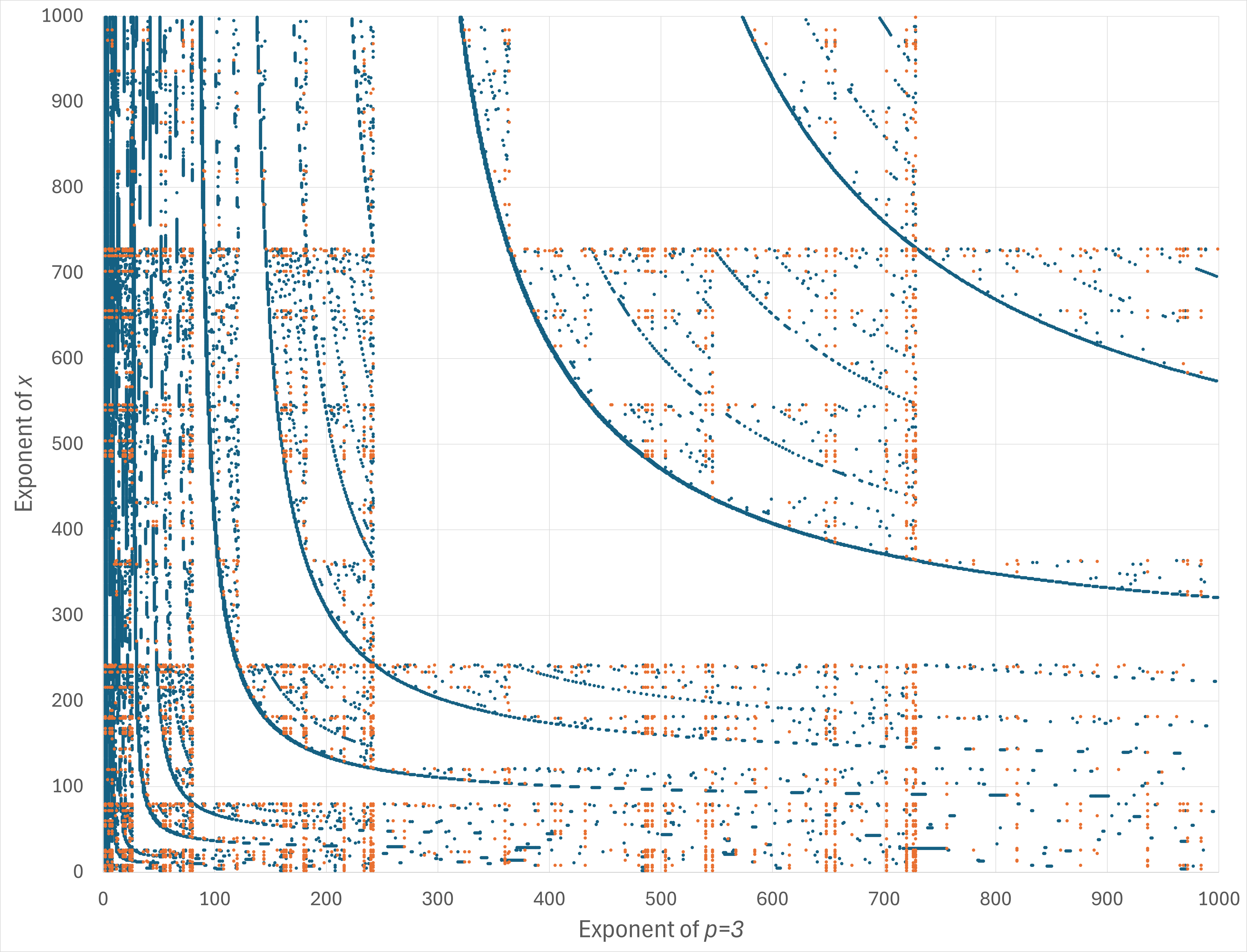
Figure 1. Values of $(a,b)$ where we know $\operatorname{+pt}(p^{a}+x^{b})$ when $p=3$. The orange dots correspond to the $a$ and $b$ values where $\operatorname{{fpt}}(f_{0})={1\over a}+{1\over b}$. The remaining dots are consequences of Section 3.

The code to generate this data set is included as an ancillary file to the arXiv version of this document and is also available on Schwede’s website.

https://www.math.utah.edu/~schwede/M2/MakeTable-PPT.m2

The code is written in Macaulay2 [GS] and uses the FrobeniusThresholds package [HSTW21].

In Section 4, we study more sporadic examples not covered in our main theorem. First, we show that if $f=x^{2}+y^{3}\in{\bf{Z}}_{2}\llbracket x,y\rrbracket=R$, then $\operatorname{+pt}(R,f)>1/2=\operatorname{{fpt}}(x^{2}+y^{3}\in{\bf F}_{2}\llbracket x,y\rrbracket)$, see Section 4.1. In Section 4.2, we study the $\operatorname{+pt}$ of the analog of “three lines”, $px(x-p)\in{\bf{Z}}_{p}\llbracket x\rrbracket$, showing it agrees with the $\operatorname{{fpt}}$ of the analogous three lines. Finally, in Section 4.3 we show that the plus-pure threshold of $2^{a}+x^{2}\in{\bf Z}_{2}[\![x]\!]$ is $1/2$ for all integers $a\geq 2$.

Acknowledgments

The authors thank Linquan Ma for valuable discussions and comments on a previous draft. In particular, Linquan Ma pointed out that Section 4.1 holds for arbitrary big Cohen-Macaulay algebras (and not just $R^{+}$) which then shows Section 4.1. This material is partly based upon work supported by the National Science Foundation under Grant No. DMS-1928930 and by the Alfred P. Sloan Foundation under grant G-2021-16778, while the authors were visiting the Simons Laufer Mathematical Sciences Institute (formerly MSRI) in Berkeley, California, during the Spring 2024 semester. Hanlin Cai was partially supported by NSF FRG Grant #1952522. Pande was partially supported by NSF Grant #2101075. Quinlan-Gallego was partially supported by an NSF Postdoctoral Research Fellowship #2203065. Schwede was partially supported by NSF Grant #2101800 and by NSF FRG Grant #1952522. Tucker was partially supported by NSF Grant #2200716.

2. Preliminaries

As usual, a prime number $p>0$ is fixed.

2.1. Plus pure thresholds

Recall a commutative integral domain $S$ is said to be absolutely integrally closed if every monic polynomial in $S[T]$ splits into a product of linear factors or, equivalently, if every monic polynomial with coefficients in $S$ has a solution in $S$. Given an arbitrary integral domain $R$ with fraction field $K$, after fixing an algebraic closure $\overline{K}$ of $K$, the integral closure $R^{+}$ of $R$ in $\overline{K}$ is an absolutely integrally closed domain, called the absolute integral closure of $R$.

If $S$ is an absolutely integrally closed domain and $z\in S$ is an element, given a nonnegative rational number $\alpha=n/m$ with $n,m\in{\bf Z}$, we let $z^{\alpha}\in S$ denote a choice of element for which $(z^{\alpha})^{m}=z^{n}$. Note that up to units such a choice of $z^{\alpha}$ is unique and independent of the representation $\alpha=n/m$. We will be sloppy about the nonuniqueness: in general we will only make statements about the membership of $z^{\alpha}$ in some ideal of $R^{+}$ or statements about ideals in which $z^{\alpha}$ is a generator. Such statements are, of course, independent of the choice of $z^{\alpha}$.

Definition 2.1.

Suppose $(S,\mathfrak{m})$ is a complete Noetherian local domain of residue characteristic $p>0$. We suppose further that $0\neq f\in\mathfrak{m}$. In this case we define the plus-pure-threshold of $f$ to be

$$\operatorname{+pt}(f):=\sup\big{\{}\alpha\in{\bf Q}_{\geq 0}\;\big{|}\;S\xrightarrow{1\mapsto f^{\alpha}}S^{+}\;\text{ is pure}\big{\}}$$

We write down some equivalent ways to check the purity of the map $S\xrightarrow{1\mapsto f^{\alpha}}S^{+}$.

Lemma 2.2.

With notation as in Section 2.1 suppose additionally that $S$ is regular, $\alpha\in{\bf Q}_{\geq 0}$, and $f^{\alpha}\in S^{+}$ is fixed. Then the following is equivalent.

1. The map $S\xrightarrow{1\mapsto f^{\alpha}}S^{+}$ is pure (equivalently splits).

2. If $E$ is an injective hull of $S/\mathfrak{m}$, then the induced map $S\otimes_{S}E\xrightarrow{1\mapsto f^{\alpha}}S^{+}\otimes_{S}E$ is injective.

3. The map $S\xrightarrow{1\mapsto f^{\alpha}}\widehat{S^{+}}$ is pure (equivalently splits) where $\widehat{S^{+}}$ is the $p$-adic (or $\mathfrak{m}$-adic) completion of $S^{+}$.

4. For each finite extension $S\subseteq S^{\prime}\subseteq S^{+}$ containing $f^{\alpha}$ we have that

   $$S\xrightarrow{1\mapsto f^{\alpha}}S^{\prime}$$

   splits.

5. $f^{\alpha}\notin\mathfrak{m}S^{+}$.

6. $f^{\alpha}\notin\mathfrak{m}\widehat{S^{+}}$ where $\widehat{S^{+}}$ is the $p$-adic (or $\mathfrak{m}$-adic) completion of $S^{+}$

7. $\tau_{+}(S,f^{\alpha})=S$ where $\tau_{+}(S,f^{\alpha})=\tau_{+}(S,\alpha\operatorname{{div}}(f))$ is the plus-test-ideal denoted as $\tau_{\widehat{R^{+}}}(S,f^{\alpha})$ in [MS21], see also [BMP⁺23a, Definition 4.16], [HLS24, Section 4] (setting $X=\operatorname{{Spec}}S$), or [BMP⁺23b, Section 8].

Proof.

In parts (i) and (iii) we see that the “equivalently splits” statements are harmless as $S$ is complete so that pure and split maps from $S$ are equivalent, see [Fed83, Lemma 1.2]. The equivalence of (i) and (ii) follows easily from Matlis duality, see [HH95, Lemma (2.1)(e)]. Then the equivalence of (i) and (iii) follows from the fact that $\widehat{S^{+}}\otimes_{S}E\simeq S^{+}\otimes_{S}E$ so we win by using (ii). Certainly (iv) and (i) are equivalent since a filtered colimit of split maps is pure [Sta, Tag 058H].

So far, we have not used regularity, but we need it for the next two statements. Clearly, (v) and (vi) are equivalent since $p\in\mathfrak{m}$. Therefore, it suffices to prove the equivalence of (vi) and (ii). If $f^{\alpha}\in\mathfrak{m}\widehat{S^{+}}$, then $S\longrightarrow\widehat{S^{+}}$ is not pure by tensoring with $k$. Conversely, assume that $f^{\alpha}\notin\mathfrak{m}\widehat{S^{+}}$. Since $S$ is regular, $\widehat{S^{+}}$ is big Cohen-Macaulay and so is faithfully flat over $S$ by [HH92, Page 77] or [Bha20, Lemma 2.9]. Hence the injectivity of $k\longrightarrow E$ extends to the injectivity of $k\otimes_{S}\widehat{S^{+}}\longrightarrow E\otimes_{S}\widehat{S^{+}}$, giving the injectivity of $k\longrightarrow E\otimes_{S}\widehat{S^{+}}$. By considering the socle, we have $E\longrightarrow E\otimes_{S}\widehat{S^{+}}$ being injective as desired.

Unraveling the definition of $\tau_{+}(S,f^{\alpha})$ easily implies it is equivalent to many of the other definitions above. More precisely, since $\tau_{+}(S,f^{\alpha})$ is the Matlis dual of the image of $S\otimes_{S}E\longrightarrow S^{+}\otimes_{S}E$, $\tau_{+}(S,f^{\alpha})=S$ if and only if $S\otimes_{S}E\longrightarrow S^{+}\otimes_{S}E$ is injective.∎

2.2. Ideal containments

Lemma 2.3.

Let $S$ be an absolutely integrally closed domain, let $z,y,y_{1},\dots,y_{s}\in S$ be elements, let $e\geq 1$ be an integer and $\epsilon\in{\bf Q}$ be a rational number.

1. If $\epsilon\in(0,\frac{p}{p-1}]$ then we have

   $$z\in(p^{\epsilon},y)\;\Longleftrightarrow\;z^{1/p^{e}}\in(p^{\epsilon/p^{e}},y^{1/p^{e}}).$$

2. If $\epsilon\in(0,1]$, we have

   $$z\in(p^{\epsilon},y_{1},\dots,y_{s})\;\Longleftrightarrow\;z^{1/p^{e}}\in(p^{\epsilon/p^{e}},y_{1}^{1/p^{e}},\dots,y_{s}^{1/p^{e}}).$$

3. If $\epsilon\in(0,1]$ and $\gamma\in\frac{1}{p^{e}}{\bf Z}\cap(0,1)$ then we have

   $$z\in(p^{\epsilon},y_{1},\dots,y_{s})\implies z^{\gamma}\in\bigg{(}p^{\epsilon\alpha_{0}}y_{1}^{\alpha_{1}}\cdots y_{s}^{\alpha_{s}}\ \bigg{|}{{\alpha_{i}\in\frac{1}{p^{e}}{\bf Z}\cap(0,1)}\atop{\alpha_{0}+\cdots+\alpha_{s}=\gamma}}\bigg{)}$$

These for $\epsilon\leq 1$ results can be deduced from [Sch12, Proposition 5.5] as the $p$-adic completion of an absolutely integrally closed domain is perfectoid. We provide a direct and down-to-earth proof for the convenience of the reader.

Proof.

We start with statement (i), and we observe that it is enough to prove it in the case $e=1$. For the $(\Longrightarrow)$ direction, after replacing $y$ with a multiple we may assume that $z=ap^{\epsilon}+y$ for some $a\in S$, and we look for elements $s\in S$ satisfying $z^{1/p}=sp^{\epsilon/p}+y^{1/p}$ or, in other words,

$$ap^{\epsilon}+y =(sp^{\epsilon/p}+y^{1/p})^{p}$$

$$=sp^{\epsilon}+p^{1+(\epsilon/p)}\big{(}\cdots\big{)}+y.$$

The assumption on $\epsilon$ ensures that $\epsilon\leq 1+(\epsilon/p)$, and therefore after canceling the $y$ terms one can divide the above equation by $p^{\epsilon}$, which ensures that the resulting equation on $s$ is monic. Since $S$ is absolutely integrally closed by assumption, there are elements $s\in S$ satisfying the required equation.

For the $(\Longleftarrow)$ direction, after replacing $y$ with a multiple we may assume that $z^{1/p}=sp^{\epsilon/p}+y^{1/p}$ for some $s\in S$, and the equation above gives $z\in(p^{\epsilon},y)$.

As before, it suffices to prove statement (ii) in the case $e=1$, and we begin with the $(\Longrightarrow)$ direction. After replacing the $y_{i}$ with multiples, we may assume $z$ takes the form $z=ap^{\epsilon}+y_{1}+\cdots+y_{s}$ for some $a\in S$, and we now look for $s\in S$ satisfying $z^{1/p}=sp^{\epsilon/p}+y_{1}^{1/p}+\cdots+y_{s}^{1/p}$ or, in other words,

$$ap^{\epsilon}+y_{1}+\cdots+y_{s} =(sp^{\epsilon/p}+y_{1}^{1/p}+\cdots+y_{s}^{1/p})^{p}$$

$$=sp^{\epsilon}+p\big{(}\cdots\big{)}+y_{1}+\cdots+y_{s},$$

which once again turns into a monic equation on $s$ after cancellation and division by $p^{\epsilon}$. The $(\Longleftarrow)$ direction also follows from a direct argument, as in part (i).

Next we prove (iii). The assumptions on $\gamma$ mean that we can write $\gamma=c_{1}p^{-1}+c_{2}p^{-2}+\cdots+c_{e}p^{-e}$ for some integers $c_{i}$ with $0\leq c_{i}\leq p-1$. Using part (ii), we then obtain

$$z^{\gamma}=\prod_{i=1}^{e}(z^{1/p^{i}})^{c_{i}}\in\prod_{i=1}^{e}(p^{\epsilon/p^{i}},y_{1}^{1/p^{i}},\dots,y_{s}^{1/p^{i}})^{c_{i}}$$

Note that the $i$-th factor in the above product of ideals is generated by the monomials

$$p^{\epsilon a_{i0}/p^{i}}y_{1}^{a_{i1}/p^{i}}\cdots y_{s}^{a_{is}/p^{i}}$$

as the $a_{ij}$ range through all nonnegative integers with $\sum_{j}a_{ij}=c_{i}$. We conclude that the product is generated by elements of the form

$$p^{\epsilon\sum a_{0i}/p^{i}}\ y_{1}^{\ \sum a_{i1}/p^{i}}y_{2}^{\ \sum a_{i2}/p^{i}}\cdots\ y_{s}^{\ \sum a_{is}/p^{i}},$$

and by setting $\alpha_{j}=\sum_{i}a_{ij}/p^{i}$, we see that all of these are contained in the ideal given. ∎

Remark 2.4.

In statement (iii) above, the proof gives an even stronger statement: whenever we have $z\in(p^{\epsilon},y_{1},\dots,y_{s})$ we can conclude that $z^{\gamma}$ belongs to the ideal generated by the monomials $p^{\epsilon\alpha_{0}}y_{1}^{\alpha_{1}}\cdots y_{s}^{\alpha_{s}}$ as above, where we impose the extra condition that the $\alpha_{i}$ add up to $\gamma$ with no carries in base $p$.

Lemma 2.5.

Let $k$ be a perfect field of characteristic $p>0$, and consider $R\colonequals k\llbracket u,x\rrbracket$ a formal power series ring in two variables over $k$. Given integers $a,b\geq 2$ , an integer $\ell\geq 1$, and a real number $t>0$, we have

$$(R,u^{1-1/a}x^{1-1/b}(u^{\ell}+x^{\ell})^{t})\text{ is $F$-regular}\;\Longleftrightarrow\;(R,(u^{a\ell}+x^{b\ell})^{t})\text{ is $F$-regular.}$$

We give two proofs. First, we point out this is a consequence of general theorems about the behavior of $F$-singularities under finite maps. For the second, we do a down-to-earth computation.

Proof #1.

Consider the extension $A=k\llbracket u^{\prime},x^{\prime}\rrbracket=k\llbracket u^{a},x^{b}\rrbracket\subseteq k\llbracket u,x\rrbracket=R$ with induced map $g$ on $\operatorname{{Spec}}$. We know that $(R,u^{1-1/a}x^{1-1/b}(u^{\ell}+x^{\ell})^{t})$ is strongly $F$-regular if and only if

(1) $$\Big{(}A,{a-1\over a}\operatorname{{div}}(u^{\prime})+{b-1\over b}\operatorname{{div}}(x^{\prime}),(u^{\prime\ell}+x^{\prime\ell})^{t}\Big{)}$$

is. Consider the map $\mathbb{T}:k[u,x]\longrightarrow k[u^{\prime},x^{\prime}]$ sending $1$ to $1$ and the other monomial basis elements to zero. The associated ramification-like-divisor is $\scr{R}_{\mathbb{T}}:=(a-1)\operatorname{{div}}(u)+(b-1)\operatorname{{div}}(x)$ as in [ST14]. As

$$g^{*}\big{(}{a-1\over a}\operatorname{{div}}(u^{\prime})+{b-1\over b}\operatorname{{div}}(x^{\prime})\big{)}-\scr{R}_{\mathbb{T}}=0$$

by [ST14, Theorem 6.25], we see that

$$\mathbb{T}\big{(}\tau(R,(u^{a\ell}+x^{b\ell})^{t})\big{)}=\tau\big{(}A,{a-1\over a}\operatorname{{div}}(u^{\prime})+{b-1\over b}\operatorname{{div}}(x^{\prime}),(u^{\prime\ell}+x^{\prime\ell})^{t}\big{)}.$$

Hence, $(R,(u^{a\ell}+x^{b\ell})^{t})$ being strongly $F$-regular implies that so is (missing), as $\mathbb{T}$ surjects. The converse follows via an argument of [CR17] as $\mathbb{T}$ sends the maximal ideal of $R$ into the maximal ideal of $A$. Indeed, if $\tau(R,(u^{a\ell}+x^{b\ell})^{t})$ is contained in the maximal ideal of $R$, then its image is in the maximal ideal of $A$. ∎

Proof #2.

Since we work over a regular ring, the pair on the left is $F$-regular precisely when there is some integer $e\geq 0$ for which the map $R\longrightarrow F^{e}_{*}R$ given by $F^{e}_{*}u^{\lceil p^{e}(1-1/a)\rceil}x^{\lceil p^{e}(1-1/b)\rceil}(u^{\ell}+x^{\ell})^{\lceil p^{e}t\rceil}$ splits. We may assume that $t\in(0,1)$, in which case the splitting can only fail at the maximal ideal $(u,x)$. Using that $u,x$ form a regular sequence, we conclude that the pair on the left is $F$-regular if and only if

$$(u^{\ell}+x^{\ell})^{\lceil tp^{e}\rceil}\notin(u^{\lfloor p^{e}/a\rfloor},x^{\lfloor p^{e}/b\rfloor})$$

Now let $\tilde{R}\colonequals k[\tilde{u},\tilde{x}]$ be a new polynomial ring, and consider the $k$-algebra homomorphism $\varphi:R\longrightarrow\tilde{R}$ given by $\varphi(u)=\tilde{u}^{a}$ and $\varphi(x)=\tilde{x}^{b}$. Note that $\varphi(u^{\ell}+x^{\ell})=\tilde{u}^{a\ell}+\tilde{x}^{b\ell}$ and that for every integer $e\geq 0$ we have

$$(u^{\lfloor p^{e}/a\rfloor},x^{\lfloor p^{e}/b\rfloor})=\varphi^{-1}\big{(}(\tilde{u}^{p^{e}},\tilde{x}^{p^{e}})\big{)}.$$

We conclude that the pair on the left is $F$-regular if and only if

$$(\tilde{u}^{a\ell}+\tilde{x}^{b\ell})^{\lceil tp^{e}\rceil}\notin(\tilde{u}^{p^{e}},\tilde{x}^{p^{e}})$$

for some integer $e\geq 0$. This is, in turn, equivalent to the $F$-regularity of the pair on the right. ∎

Remark 2.6.

Proof #1 also works in mixed characteristic for a slightly different statement. It shows that $A={\bf{Z}}_{p}\llbracket x\rrbracket$ and $R=A[p^{1\over a},x^{1\over b}]$ then

$$\text{$(A,p^{1-1/a}x^{1-1/b}(p^{\ell}+x^{\ell})^{t})$ is $+$-(or BCM-)regular }\Longleftrightarrow\text{ $(R,((p^{{1\over a}})^{a\ell}+(x^{1\over b})^{b\ell})^{t})$ is $+$-(or BCM-)regular.}$$

The point is we have transformation rules for $+$-test ideals and BCM-test ideals by [MS21].

We now study a particular blowup of our singularity looks like.

Lemma 2.7.

Suppose $(R,\mathfrak{m}=(u,x),k)$ is a complete regular 2-dimensional local ring and consider $f=u^{\ell a}+x^{\ell b}\in R$ where $a$ and $b$ relatively prime. Let $\pi:X\longrightarrow\operatorname{{Spec}}R$ be the normalized blowup of the ideal $(u^{a},x^{b})$. Set $D$ to be the strict transform of $\operatorname{{div}}(f)$ on $Y$. Then we have the following.

1. $X$ has a unique reduced exceptional divisor $E\cong\mathbb{P}^{1}_{k}$.

2. $-E$ is a $\pi$-ample Weil divisor.

3. $K_{X/R}=(a+b-1)E$ and $\operatorname{{div}}(f)$ pulls back to $D+(\ell ab)E$.

4. The different of $K_{X}+E$ restricted to $E$ is $(1-{1\over a})P_{1}+(1-{1\over b})P_{2}$ for some points $P_{1},P_{2}$ on $E$.

5. $D$ intersects $E$ at nonsingular points of $Y$ (in particular, away from $P_{1}$ and $P_{2})$. Explicitly, we consider the homogeneous coordinate ring $k[y,z]$ for $E$ with $V(y)=P_{1}$ and $V(z)=P_{2}$ ($0$ and $\infty$), then we have that $D$ restricted to $E$ is given by the equation $(y^{\ell}+z^{\ell})$.

This lemma shows that the normalized blowup of $(u^{a},x^{b})$ behaves exactly as one expects from the toric setting. Those willing to believe that may wish to skip the proof on first reading.

Proof.

Consider the finite extension $S=R[u^{1\over b},x^{1\over a}]$ of $R$ (with maximal ideal $\mathfrak{n}\subseteq S$) and consider the map $\varphi:S\longrightarrow R$ sending $1$ to $1$ and the other natural basis elements $u^{i/b}x^{j/a}\mapsto 0$ for $0\leq i<b$ and $0\leq j<a$. Consider the maximal ideal $\mathfrak{n}=(u^{1/b},x^{1/a})S\subseteq S$ and notice that

$$\mathfrak{n}^{ab}\cap R=\varphi(\mathfrak{n}^{ab})=(u^{i}x^{j}\;|\;i,j\geq 0,ib+ja\geq ab)=:J.$$

As $\mathfrak{n}^{ab}$ is a valuation ideal (associated to blowing up the origin), we see that so is $J\subseteq R$. In particular, $J$ is integrally closed. As $R$ is regular and 2-dimensional, $J^{n}$ is also integrally closed for all $n$ by a result of Zariski, see [HS06, Theorem 14.4.4]. Let $X$ denote the blowup of $J$, and $Y$ the blowup of $\mathfrak{n}^{ab}$ (which is the same as the blowup of $\mathfrak{n}$, although the induced relatively very ample divisors have different coefficients), and there is a finite map $\beta:Y\longrightarrow X$ induced by the inclusion of Rees algebras $R[Jt]\subseteq S[\mathfrak{n}^{ab}t]$. Note $\varphi$ extends to these Rees algebras and hence also induces $\varphi:f_{*}\mathcal{O}_{Y}\longrightarrow\mathcal{O}_{X}$. It easily follows that $Y$ is smooth, $X$ is normal and Cohen-Macaulay (it is a summand of $f_{*}\mathcal{O}_{Y}$), and since $Y$ has a unique reduced exceptional divisor $E_{Y}$, we have that $X$ has a unique reduced exceptional divisor $E$. We have the following diagram.

On $K(S)=K(Y)$, the exceptional divisor induces a discrete valuation $v:K(S)^{\times}\longrightarrow{\bf{Z}}$ which takes $u^{1\over b}\mapsto{1},x^{1\over a}\mapsto{1}$, and sends units to $0$ (it can also be viewed as the $\mathfrak{n}$-adic order on $S$). Consider a monomial $g=u^{i}x^{j}=(u^{1\over b})^{ib}(x^{1\over a})^{ja}\in R$. Notice that $v(g)=ib+ja$. Therefore, as $a,b$ are relatively prime, there exist monomials $h\in K(R)$ with $v(h)=1$.

We consider the charts of $X$ and $Y$ corresponding to $u^{a}$ and $x^{b}$, which we label $X_{u}$, $Y_{u}$, $X_{x}$, and $Y_{x}$ respectively. As it is easy to see that $Y_{u}=\operatorname{{Spec}}S[x^{1\over a}/u^{1\over b}]=\operatorname{{Spec}}S[u^{i\over b}x^{j\over a}\;|\;i+j\geq 0,j\geq 0]=\operatorname{{Spec}}S^{u}$, one applies $\varphi$ and sees that $X_{u}=\operatorname{{Spec}}R[u^{i}x^{j}\;|\;ib+ja\geq 0,j\geq 0]=\operatorname{{Spec}}R^{u}$. Similarly $X_{x}=\operatorname{{Spec}}R[u^{i}x^{j}\;|\;ib+ja\geq 0,i\geq 0]=\operatorname{{Spec}}R^{x}$.

On $Y_{u}$, the exceptional divisor $E_{Y}$ is defined by the principal ideal $(u^{1\over b})$. As $x^{1\over a}/u^{1\over b}$ is in the ring $S^{u}$, $(u^{1\over b})S^{u}$ is also generated as a module over $R$ by the monomials $(u^{i\over b}x^{j\over a}\;|\;i+j>0)S$ (and the analogous result holds for $Y_{x}$). Hence, applying $\varphi$ on $X_{u}$ (respectively $X_{x}$) or using the valuation $v$, the ideal defining $E$ is generated by the following monomials, even using scalars from $R$,

$$I_{E,u}=(u^{i}x^{j}\in R^{u}\;|\;bi+aj>0)R\;\;\;(\text{respectively }\;I_{E,x}=(u^{i}x^{j}\in R^{x}\;|\;bi+aj>0)R).$$

A direct computation now easily implies that the exceptional divisor $E$ is isomorphic to $\mathbb{P}^{1}_{k}$. Indeed, $x^{b}/u^{a}\notin I_{E,u}$, and it is not difficult to see that $R^{u}/I_{E,u}\cong k[x^{b}/u^{a}]$, while $R^{x}/I_{E,x}\cong k[u^{a}/x^{b}]$. By construction, $E$ is an anti-ample Weil divisor. In particular, we see that (i) and (ii) hold.

We observed above that the valuation ring $T\subseteq K(R)$ associated to $E$ (or equivalently to $v|_{K(R)}$) has elements $h$ of value $1$. Set $T_{Y}\subseteq K(S)$ to be the valuation ring associated to $v$ (equivalently, associated to $E_{Y}$). Hence $T\subseteq T_{Y}$ have a common monomial uniformizer $h$ but has an extension of residue fields. Note $\varphi:T_{Y}\longrightarrow T$ sends monomials of $T$ to themselves and is nonzero on the associated residue field extension. We see thus that the divisor associated to $\varphi\in\operatorname{Hom}_{T}(T^{\prime},T)=\omega_{T^{\prime}/T}$ has coefficient zero along $E$.

We now compute canonical divisors. If we set $K_{R}=-\operatorname{{div}}(u)-\operatorname{{div}}(x)$, then associated to the map $\varphi\in\operatorname{{\scr{H}}om}(S,R)$ we obtain an effective divisor $K_{S/R}={b-1\over b}\operatorname{{div}}(u^{1\over b})+{a-1\over a}\operatorname{{div}}(x^{1\over a})$ (this is the ramification divisor if $p$ is relatively prime to $a$ and $b$, otherwise it can be thought of as a replacement for the ramification divisor, see [ST14] for related discussion). We can then set $K_{S}=\alpha^{*}K_{R}+K_{S/R}=-\operatorname{{div}}(u^{1\over b})-\operatorname{{div}}(x^{1\over a})$. Associated to the blowup $\pi_{Y}$, we see that $K_{Y}=-E_{Y}-D_{1}-D_{2}$ where $D_{1}$ and $D_{2}$ are the strict transforms of $\operatorname{{div}}(u^{1\over b})$ and $\operatorname{{div}}(x^{1\over a})$. Viewing $\varphi\in\operatorname{{\scr{H}}om}(f_{*}\mathcal{O}_{Y},\mathcal{O}_{X})$, we then obtain that $K_{Y/X}={b-1\over b}D_{1}+{a-1\over a}D_{2}+0E_{Y}$ where coefficient of $E$ was computed above. From the formula $K_{Y}=K_{Y/X}+\beta^{*}K_{X}$ we see that $K_{X}=-E-D_{x}-D_{u}$ where $D_{x}$ and $D_{y}$ are the strict transforms of $\operatorname{{div}}(x)$ and $\operatorname{{div}}(u)$. This is what is expected based on the toric setting.

For (iii), we compute the relative canonical and the pullback of $\operatorname{{div}}(f)$. Observe that

$$\begin{array}[]{rl}\beta^{*}K_{X/R}=&\beta^{*}\big{(}K_{X}-\pi^{*}(-\operatorname{{div}}(ux))\big{)}\\ =&\beta^{*}(-E-D_{x}-D_{u})+\pi_{Y}^{*}(a\operatorname{{div}}(u^{1\over a})+b\operatorname{{div}}(b^{1\over b}))\\ =&-E_{Y}-aD_{1}-bD_{2}+{a+b}E_{Y}-aD_{1}-bD_{2}\\ =&(a+b-1)E_{Y}\end{array}$$

As $\beta^{*}E=E_{Y}$, this implies that $K_{X/R}=(a+b-1)E$. Next, we compute the pullback of $\operatorname{{div}}(f)$. By pulling back to $Y$ and employing a similar argument, we see that $\pi^{*}\operatorname{{div}}(f)=(\ell ab)E+D$.

We can now compute the different. Note, $K_{X}+E$ has coefficient zero along $E$ and so it suffices to compute $(K_{X}+E)|_{E}\sim_{{\bf Q}}K_{E}+\mathrm{Diff}$ in a specific way. We do our computation on the chart $U:=X_{u}$ as the other chart is similar. First, we can pick a section $s=x^{b}/u^{a}\in\mathcal{O}_{U}(K_{X}+E)$. This produces a divisor $D_{s}=(b-1)D_{x}|_{U}\sim(K_{X}+E)|_{U}$ on this chart. Consider the image of this section $\overline{s}$ under the canonical map $\omega_{U}(E)\twoheadrightarrow\omega_{E}$. Viewing these as ideal sheaves, we see that while $s$ does not generate $\omega_{U}(E)=\mathcal{O}_{U}(-D_{x})$, its image generates the image of $\omega_{E}$ of $\omega_{U}(E)$, which is the ideal $(x^{b}/u^{a})\in k[x^{b}/u^{a}]$. Therefore, we see that the associated divisor $D_{\overline{s}}=0\sim K_{E}$. The different is thus computed as

$$(D_{s})|_{E}=D_{\overline{s}}+{\mathrm{Diff}}.$$

As $D_{s}=(b-1)D_{x}|_{U}={b-1\over b}\operatorname{{div}}(x^{b}/u^{a})$ we see that the different $\operatorname{Diff}$ is ${b-1\over b}P_{1}$ where $P_{1}=D_{1}\cap E$ (the origin in this chart). The analogous computation shows that on the other chart, the different is ${a-1\over a}P_{2}$. This proves (iv).

For the final statement (v), we simply need to understand how $D$, the strict transform of $\operatorname{{div}}(f)$, restricts to $E\cong\mathbb{P}^{1}_{k}$. We again work on the chart $U=X_{u}$ and observe $f=u^{\ell a}+x^{\ell b}=u^{\ell a}\big{(}1+({x^{b}\over u^{a}})^{\ell}\big{)}$. As $1+({x^{b}\over u^{a}})^{\ell}$ does not vanish along the exceptional divisor, we see it must be the equation of the strict transform. As the analogous result holds on the chart $X_{x}$, the result follows. ∎

Proposition 2.8.

Let $R\colonequals{\bf Z}_{p}[\![x]\!]$, let $a,b\geq 2$ be integers, and consider the polynomial $f\colonequals p^{a}+x^{b}\in R$. Consider $R_{0}\colonequals{\bf F}_{p}[\![y,x]\!]$ and $f_{0}\colonequals y^{a}+x^{b}\in R_{0}$. Then we have

$$\operatorname{{fpt}}(R_{0},f_{0})\leq\operatorname{+pt}(R,f)\leq{1\over a}+{1\over b}.$$

Proof.

We may replace $a$ by $\ell a$ and $b$ by $\ell b$ where $\ell=\gcd(a,b)$ so that $a$ and $b$ are relatively prime. Consider the normalized blowup $\pi:X\longrightarrow\operatorname{{Spec}}R$ of $(p^{a},x^{b})$ as in Section 2.2. Note, every $+$-regular pair is automatically KLT by [MS21, Theorem 6.21] ($\widehat{R^{+}}$ is big enough for that containment), or use Matlis duality and [BMP⁺23a, Definition 4.16]. Hence, the computation of Section 2.2 (iii) implies that

$$\operatorname{+pt}(f)\leq\sup\{t\;|\;a+b-1-t\ell ab>-1\}={1\over\ell a}+{1\over\ell b}$$

as desired. Indeed, it is not hard to see that this is the log canonical threshold.

For the other inequality, let $E$ be the exceptional divisor of $\pi$ and let $D$ denote the strict transform of $\operatorname{{div}}(f)$. Suppose now that $t<\operatorname{{fpt}}(f_{0})$. By Section 2.2, we see that $t<\operatorname{{fpt}}(R_{0},y^{1-1/a}x^{1-1/b}(u^{\ell}+x^{\ell})^{t})$. Using Section 2.2 (iv) and (v), we see that $(E,\operatorname{Diff}_{E}(tD))$ has a section ring whose associated pair is $(R_{0},y^{1-1/a}x^{1-1/b}(u^{\ell}+x^{\ell})^{t})$. In particular, $(E,(K_{X}+E+tD)|_{E})$ is globally $F$-regular and so [MST⁺22, Lemma 7.2] implies that $(R,f^{t})$ is $+$-regular (this also follows from [BMP⁺23a, Theorem 7.2]). The result follows. ∎

Remark 2.9.

One can also use direct computation to prove that $\operatorname{+pt}\leq{1\over a}+{1\over b}$. We sketch this here.

Let $\zeta\in R^{+}$ be a primitive $(2ab)$-th root of unity, let $e\geq 0$ be an integer and $\gamma\in\frac{1}{p^{e}}{\bf Z}$ be a rational number whose denominator is $p^{e}$. We then have

$$f^{\gamma}=(p^{ab/b}+x^{ab/a})^{\gamma} =\prod_{i=0}^{ab-1}(p^{1/b}-\zeta^{i}x^{1/a})^{\gamma}.$$

Since for every $i=0,\dots,ab-1$ we have $(p^{1/b}-\zeta^{i}x^{1/a})\in(p^{1/b},x^{1/a})$, by Section 2.2, we conclude that

$$f^{\gamma}\in\bigg{(}p^{\beta/b}x^{\alpha/a}\ \bigg{|}\ {{\alpha,\beta\in\frac{1}{p^{e}}{\bf Z}}\atop{\alpha+\beta=\gamma}}\bigg{)}^{ab}\subseteq\bigg{(}p^{\beta/b}x^{\alpha/a}\ \bigg{|}\ {{\alpha,\beta\in\frac{1}{p^{e}}{\bf Z}}\atop{\alpha+\beta=ab\gamma}}\bigg{)}.$$

Therefore, whenever $\gamma\geq(1/a)+(1/b)$ we have $ab\gamma\geq a+b$, and hence every choice of $\alpha,\beta$ with $\alpha+\beta=ab\gamma$ must have $\alpha\geq a$ or $\beta\geq b$, and hence $f^{\gamma}\in(p,x)R^{+}$.

Remark 2.10.

Suppose $F\in{\bf{Z}}[x,y]$ is homogeneous of degree $d$, $f:=F(p,y)\in{\bf{Z}}_{p}\llbracket y\rrbracket=R$, and $f_{0}:=F(x,y)\in{\bf F}_{p}\llbracket x,y\rrbracket$. Let $X\longrightarrow\operatorname{{Spec}}{\bf{Z}}_{p}\llbracket y\rrbracket$ denote the blowup of the origin with exceptional divisor $E$. On the chart $\operatorname{{Spec}}R[y/p]$ corresponding to $p$, $f=p^{d}F(1,y/p)$. On $E=V(p)$, the strict transform defined by $F(1,y/p)$ restricts to a divisor defined by $f_{0}(1,x/y)$. Likewise on the chart corresponding to $x$, $f=x^{d}F(1,p/x)$. Restricting the strict transform defined by $F(1,p/x)$ to $E=V(x)$, we get $F(1,y/x)$. Putting this together, we see that the strict transform of $\operatorname{{div}}(f)$ intersects the exceptional $\mathbb{P}^{1}$ in $V(f_{0})$ (viewed as a homogeneous equation).

The argument of Section 2.2 then implies that

$$\operatorname{{fpt}}(R_{0},f_{0})\leq\operatorname{+pt}(R,f)\leq\min\{t\;|\;1-td>-1\}={2\over d}.$$

In fact, the argument is easier as there is no additional contribution to the different to worry about (that is, Section 2.2 is unnecessary).

As a consequence, we see that the extremal bounds of [KKP⁺22] also apply in mixed characteristic. Analogous computations can also be done in higher dimension.

3. Cusp-like singularities

As usual, $p>0$ is a fixed prime number, and we let $R\colonequals{\bf Z}_{p}[\![x]\!]$ be a power series ring in one variable over ${\bf Z}_{p}$. Given integers $a,b\geq 2$ we let $f\colonequals p^{a}+x^{b}\in R$, and we let $f_{0}\colonequals t^{a}+x^{b}\in{\bf F}_{p}[\![t,x]\!]$. Recall that we have

$$\operatorname{{fpt}}(R_{0},f_{0})\leq\operatorname{+pt}(R,f)\leq\frac{1}{a}+\frac{1}{b}.$$

In particular, we have $\operatorname{+pt}(f)=(1/a)+(1/b)$ whenever $\operatorname{{fpt}}(f_{0})=(1/a)+(1/b)$. We also recall that, by [Her14], whenever $\operatorname{{fpt}}(f_{0})\neq(1/a)+(1/b)$ then the denominator of $\operatorname{{fpt}}(f_{0})$ is a power of $p$; that is, there is some integer $e\geq 1$ such that $p^{e}\operatorname{{fpt}}(f_{0})\in{\bf Z}$.

Our general goal in this section is to show that that, when $\operatorname{{fpt}}(f_{0})$ is not too far from $(1/a)+(1/b)$, then we have an equality $\operatorname{{fpt}}(f_{0})=\operatorname{+pt}(f)$. We begin by introducing some notation to set up the technical result. As usual, we assume a prime $p>0$ is fixed.

Given a real number $\lambda>0$ and an integer $e\geq 1$, we let $\rho_{e}(\lambda)$ be the largest rational number whose denominator is $p^{e}$ with the property that $\rho_{e}(\lambda)<\lambda$. This can be written out precisely as

$$\rho_{e}(\lambda)\colonequals\frac{\lceil\lambda p^{e}\rceil-1}{p^{e}}.$$

Theorem 3.1.

Let $p>0$ be a prime number and consider the ring $R\colonequals{\bf Z}_{p}[\![x]\!]$. Fix integers $a,b\geq 2$ and consider $f\colonequals p^{a}+x^{b}\in R$. Fix an integer $e\geq 1$ and a number $\gamma\in(1/p^{e}){\bf Z}\cap(0,1)$, and assume that for some integer $c\geq a-\lfloor a/p\rfloor$ one has

$$\gamma>\frac{1}{c}\left(\rho_{e}\left(\frac{c}{a}\right)+\rho_{e}\left(\frac{c}{b}\right)\right).$$

Then $f^{\gamma}\in(p,x)R^{+}$.

Proof.

Let $\zeta$ be a primitive $(2c)$-th root of unity, and note that

$$f^{\gamma}=\big{(}(p^{a/c})^{c}+(x^{b/c})^{c})=\prod_{i=0}^{c-1}(p^{a/c}+\zeta^{i}x^{b/c})^{\gamma}.$$

For every $i=0,\dots,c-1$ we have $p^{a/c}+\zeta^{i}x^{b/c}\in(p^{a/c},x^{b/c})$. Moreover, by our assumption on $c$, we have that $a/c\leq p/(p-1)$, and hence we can apply Section 2.2 to conclude that $f^{\gamma}$ belongs to the ideal of $R^{+}$ generated by monomials of the form

$$p^{(a/c)(\alpha_{1}+\cdots+\alpha_{c})}\ x^{(b/c)(\beta_{1}+\cdots+\beta_{c})},$$

where $\alpha_{1},\dots,\alpha_{c},\beta_{1},\dots,\beta_{c}\in(1/p^{e}){\bf Z}\cap[0,1)$ satisfy $\alpha_{i}+\beta_{i}=\gamma$ for all $i=1,\dots c$. Now, if $f^{\gamma}\notin(p,x)R^{+}$, then there is a choice of such $\alpha_{i}$ and $\beta_{i}$ for which $\sum\alpha_{i}<c/a$ and $\sum\beta_{i}<c/b$. Since $\sum\alpha_{i}$ and $\sum\beta_{i}$ both have denominator $p^{e}$, this gives

$$c\gamma=\sum\alpha_{i}+\sum\beta_{i}\leq\rho_{e}\left(\frac{c}{a}\right)+\rho_{e}\left(\frac{c}{b}\right),$$

contradicting the assumption on $\gamma$. ∎

Corollary 3.2.

Consider the ring $R_{0}\colonequals{\bf F}_{p}[\![y,x]\!]$ and the element $f_{0}\colonequals y^{a}+x^{b}\in R_{0}$. Assume $\operatorname{{fpt}}(R_{0},f_{0})\neq(1/a)+(1/b)$ and fix an integer $e\geq 1$ such that $p^{e}\operatorname{{fpt}}(R_{0},f_{0})\in{\bf Z}$. If there is some integer $c\geq a-\lfloor a/p\rfloor$ for which the inequality

$$\operatorname{{fpt}}(R_{0},f_{0})>\frac{1}{c}\left(\rho_{e}\left(\frac{c}{a}\right)+\rho_{e}\left(\frac{c}{b}\right)\right)$$

holds, then $\operatorname{{fpt}}(R_{0},f_{0})=\operatorname{+pt}(f)$. In particular, setting $c=a$, we get $\operatorname{{fpt}}(R_{0},f_{0})=\operatorname{+pt}(R,f)$ whenever

$$\operatorname{{fpt}}(R_{0},f_{0})\geq\frac{1}{a}+\frac{1}{b}-\frac{1}{ap^{e}}.$$

Proof.

Setting $\gamma=\operatorname{{fpt}}(R_{0},f_{0})$ in Theorem 3.1, we conclude that $\operatorname{{fpt}}(R_{0},f_{0})\geq\operatorname{+pt}(R,f)$. The reverse inequality is given by Section 2.2. ∎

It is shown in [Her14] that, given integers $a,b\geq 2$, the $F$-pure threshold of $f_{0}\colonequals t^{a}+x^{b}\in{\bf F}_{p}[\![t,x]\!]$ can be computed from the base-$p$ expansions of $1/a$ and $1/b$. We discuss this algorithm in the case where $p>ab$.

For each integer $i\geq 0$, let $x_{i}\in\{1,\dots,a-1\}$ be the standard representative of $p^{i}$ in $({\bf Z}/a)^{\times}$, so that the expansion of $1/a$ in base $p$ is

$$\frac{1}{a} =\frac{1}{p}\left(\frac{px_{0}-x_{1}}{a}\right)+\frac{1}{p^{2}}\left(\frac{px_{1}-x_{2}}{a}\right)+\frac{1}{p^{3}}\left(\frac{px_{2}-x_{3}}{a}\right)+\cdots$$

Similarly, letting $$y_{i}\in\{1,\dots,b-1\} p^{i} ({\bf Z}/b)^{\times} 1/b p$$ be the standard representative of in , the expansion of in base becomes

$$\frac{1}{b} =\frac{1}{p}\left(\frac{py_{0}--y_{1}}{b}\right)+\frac{1}{p^{2}}\left(\frac{py_{1}-y_{2}}{b}\right)+\frac{1}{p^{3}}\left(\frac{py_{2}-y_{3}}{b}\right)+\cdots.$$

Now let $m$ be the smallest integer $i\geq 0$ for which $(x_{i}/a)+(y_{i}/b)>1$, with the understanding that $m=\infty$ if this never occurs. Note that, because $x_{0}=y_{0}=1$, we always have $m\geq 1$.

This $m$ can also be thought of as follows: the sum $(1/a)+(1/b)$ first carries when performed in base $p$ at the $(m+1)$-th digit. The $F$-pure threshold of $f_{0}$ is then obtained as a suitable truncation of the sum $(1/a)+(1/b)$ in base $p$; more precisely, we have

$$\operatorname{{fpt}}(f_{0})=\frac{1}{p^{m}}+\sum_{i=1}^{m}\frac{1}{p^{i}}\left(\frac{x_{i-1}p-x_{i}}{a}+\frac{y_{i-1}p-y_{i}}{b}\right)=\frac{1}{a}+\frac{1}{b}-\frac{1}{p^{m}}\left(\frac{x_{m}}{a}+\frac{y_{m}}{b}-1\right),$$

with the understanding that this is $(1/a)+(1/b)$ if $m=\infty$.

Crucially for us, given integers $a,b\geq 2$, there exist rational numbers $C_{i}\geq 0$ and integers $m_{i}\geq 1$, indexed by $i\in({\bf Z}/ab)^{\times}$, such that for all $p>ab$ we have

$$\operatorname{{fpt}}(f_{0})=\frac{1}{a}+\frac{1}{b}-\frac{C_{i}}{p^{m_{i}}}\text{ when }p\equiv i\text{ mod }ab.$$

By virtue of Section 3, whenever we have $C_{i}\leq 1/a$ we can conclude that $\operatorname{+pt}(f)=\operatorname{{fpt}}(f_{0})$ for all primes $p>ab$ for which $p\equiv i\text{ mod }ab$. Since the computation of $\operatorname{{fpt}}(f_{0})$ is implemented in the FrobeniusThresholds package for Macaulay2 [HSTW21], we have an effective way to find primes for which we get $\operatorname{+pt}(f)=\operatorname{{fpt}}(f_{0})$; the result of such a search for $2\leq a,b\leq 5$ are displayed in Table 1 in the Introduction. Note that the full strength of Section 3 is used for testing some small primes, and that the omission of a given prime from the table does not entail that $\operatorname{+pt}(f)$ differs from $\operatorname{{fpt}}(f_{0})$—only that we do not know whether it is true.

Remark 3.3.

In Section 4 we show that $\operatorname{+pt}(R,f)=\operatorname{{fpt}}(R_{0},f_{0})$ for some other cusp-like singularities for which the hypotheses of Section 3 fail: we show that this is the case for $R\colonequals{\bf Z}_{2}[\![x]\!]$ and $f=2^{a}+x^{2}\in R$ for any $a\geq 2$.

4. Sporadic examples

In this section we explore some sporadic examples, where we make crucial use of the following lemma, which utilizes the fact that the $p$-adic completion of $R^{+}$ is Cohen Macaulay for a power series ring $R$ over the $p$-adic integers [Bha20].

Lemma 4.1.

Let $R\colonequals{\bf Z}_{p}[\![x_{1},\dots,x_{n}]\!]$ be a power series ring over the $p$-adic integers. Let $\alpha_{0},\alpha_{1},\dots,\alpha_{n}\in{\bf Q}\cap[0,1)$, and let $h\in R^{+}$. Then

$$p^{\alpha_{0}}x_{1}^{\alpha_{1}}\cdots x_{n}^{\alpha_{n}}h\in(p,x_{1},\dots,x_{n})R^{+}\implies h\in(p^{1-\alpha_{0}},x_{1}^{1-\alpha_{1}},\dots,x_{n}^{1-\alpha_{n}})R^{+}.$$

Proof.

Fix $\gamma_{i}\in{\bf{Z}}$ the denominator of $\alpha_{i}$. Consider $S=R[p^{1/\gamma_{0}},x_{1}^{1/\gamma_{1}},\dots,x_{n}^{1/\gamma_{n}}]$ also a regular ring. Suppose $p^{\alpha_{0}}x_{1}^{\alpha_{1}}\cdots x_{n}^{\alpha_{n}}h\in(p,x_{1},\dots,x_{n})R^{+}$. Then certainly $p^{\alpha_{0}}x_{1}^{\alpha_{1}}\cdots x_{n}^{\alpha_{n}}h\in(p,x_{1},\dots,x_{n})\widehat{R^{+}}$ where $\widehat{R^{+}}$ is the $p$-adic completion. As $\widehat{R^{+}}$ is big Cohen-Macaulay over $S$ by [Bha20], we see that $p^{1/\gamma_{0}},x_{1}^{\gamma_{1}},\dots,x_{n}^{1/\gamma_{n}}$ is a regular sequence on $\widehat{R^{+}}$ and so

$$h\in(p^{1-\alpha_{0}},x_{1}^{1-\alpha_{1}},\dots,x_{n}^{1-\alpha_{n}})\widehat{R^{+}}.$$

Since the ideal on the right contains $p$, the result follows. ∎

4.1. The cusp $\mathbf{x^{2}+y^{3}}$ in mixed characteristic 2

We consider an honest binomial where $p$ does not replace one of the variables.

Lemma 4.2.

Let $R\colonequals{\bf Z}_{2}[\![x,y]\!]$ be a power series ring in two variables over the 2-adic integers. Further suppose that $B$ is a big Cohen-Macaulay $R^{+}$ algebra. For $f\colonequals x^{2}+y^{3}\in R$, we have $2^{1/4}\,f^{1/2}\notin(2,x,y)B$.

We originally wrote down the proof for $B=R^{+}$ utilizing Section 4. However, Linquan Ma pointed out that our argument applies to an arbitrary big Cohen-Macaulay $B$ — a stronger statement yielding Section 4.1 below.

Proof.

Suppose $2^{1/4}\,f^{1/2}\in(2,x,y)B$ for a contradiction. Then as $B$ is big Cohen-Macaulay, we have $f^{1/2}\in(2^{3/4},x,y)B$. Fix a $y^{1/2}$ and $2^{1/4}$ in $R^{+}$ and set $g\colonequals x+y^{3/2}$. Then we have $f\equiv g^{2}\bmod{(2)B}$. This implies that $(f^{1/2}-g)^{2}\in(2)B$, and Section 2.2 gives that $f^{1/2}-g\in(2^{1/2})B$. On the other hand, we have $f^{1/2}-g\in(2^{3/4},x,y)$, and by using that $B$ is big Cohen-Macaulay again we conclude that

$$f^{1/2}-g\in(2^{1/2})B\cap(2^{3/4},x,y)B=(2^{3/4},2^{1/2}x,2^{1/2}y)B.$$

Now write $f^{1/2}=x+y^{3/2}+ax2^{1/2}+by2^{1/2}+c2^{3/4}$. Now, looking at the equation

$$(x+y^{3/2}+ax2^{1/2}+by2^{1/2}+c2^{3/4})^{2}=x^{2}+y^{3}$$

modulo $2^{3/2},x^{2},y^{2}$, we conclude that $2xy^{3/2}\in(2^{3/2},x^{2},y^{2})B$, and using that $B$ is big Cohen-Macaulay yet again gives that $1\in(2^{1/2},x,y^{1/2})B$, a contradiction. ∎

Corollary 4.3.

With notation as in Section 4.1, we have that $\tau_{+}(R,f^{1/2+\epsilon})=R$ for all $1\gg\epsilon>0$. In particular, $\operatorname{+pt}(R,f)>1/2=\operatorname{{fpt}}({\bf F}_{p}\llbracket x,y\rrbracket,f)$.

Proof.

Fix a sufficiently large perfectoid big Cohen-Macaulay $R^{+}$-algebra $B$ so that we have $\tau_{B}(R,f^{t})=\tau_{\mathrm{BCM}}(R,f^{t})$ for all $t$ in the sense of [BMP⁺23b, MS21]. In particular, enlarging $B$ does not change this mixed characteristic test ideal. As $R\xrightarrow{1\mapsto f^{1/2}}B$ splits thanks to Section 4.1, we see that $\tau_{\mathrm{BCM}}(R,f^{1/2})=R$. It follows from [MS18, Proposition 6.4] that $\tau_{\mathrm{BCM}}(R,f^{1/2+\epsilon})=R$ for all $1\gg\epsilon>0$. But we always have that

$$\tau_{\mathrm{BCM}}(R,f^{1/2+\epsilon})\subseteq\tau_{+}(R,f^{1/2+\epsilon})$$

and so the corollary follows. ∎

This suggests the following question.

Question 4.4.

Is $\operatorname{+pt}(R,f)=5/6$, or perhaps more interestingly, is it something strictly in between $1/2$ and $5/6$?

4.2. 3 lines

We consider an equation similar to an arrangement of 3 lines, but where $p$ replaces a variable.

Proposition 4.5.

Let $p>0$ be a prime number and consider the rings $R\colonequals{\bf Z}_{p}[\![x]\!]$ and $R_{0}\colonequals{\bf F}_{p}[\![t,x]\!]$. Let $f=px(p-x)$ and $f_{0}=tx(t-x)$. Then we have

$$\operatorname{+pt}(f)=\mathrm{fpt}(f_{0})=\begin{cases}2/3\text{ if }p=3\\ (2p-1)/3p\text{ if }p\equiv 2\text{ mod }3\\ 2/3\text{ if }p\equiv 1\text{ mod }3.\end{cases}$$

Proof.

By Section 2.2, it suffices to show that $\operatorname{+pt}(f)\leq\mathrm{fpt}(f_{0})$, i.e. $f^{\alpha}\in\mathfrak{m}R^{+}$ for any $\alpha\geq\mathrm{fpt}(f_{0})$. By Section 4, it suffices to show that

$$(x-p)^{\alpha}\in(p^{1-\alpha},x^{1-\alpha}).$$

Suppose $\alpha=a/p^{e}$. Then by Section 2.2, we know that

$$(x-p)^{1/p^{e}}\in(p^{1/p^{e}},x^{1/p^{e}}).$$

Hence $(x-p)^{a/p^{e}}\in(p^{1/p^{e}},x^{1/p^{e}})^{a}$. When $p\equiv 2\text{ mod }3$, we just take $a=(2p-1)/3$ and $e=1$. Then by pigeonhole principle, we have $(p^{1/p},x^{1/p})^{(2p-1)/3}\subset(p^{(p+1)/3p},x^{(p+1)/3p})$ and hence the desired containment. Otherwise, when $a/p^{e}\geq 2/3$, we still have $(p^{1/p^{e}},x^{1/p^{e}})^{a}\subset(p^{(p^{e}-a)/p^{e}},x^{(p^{e}-a)/p^{e}})$ by pigeonhole principle. ∎

4.3. The polynomial $\mathbf{2^{a}+x^{2}}$ in mixed characteristic 2.

Let $R\colonequals{\bf Z}_{2}[\![x]\!]$ be a power series ring over the 2-adic integers, let $a\geq 2$ be an integer, and consider the polynomial $f\colonequals 2^{a}+x^{2}\in R$. As usual, we consider the equal characteristic $2$ analogues $R_{0}\colonequals{\bf F}_{2}[\![y,x]\!]$ and $f_{0}\colonequals y^{a}+x^{2}\in R_{0}$. The polynomial $f$ does not always satisfy the hypotheses of Section 3 but, nonetheless, we show that $\operatorname{+pt}(R,f)=1/2=\operatorname{{fpt}}(R_{0},f_{0})$ with a more elementary argument.

Proposition 4.6.

Let $R\colonequals{\bf Z}_{2}[\![x]\!]$, $a\geq 2$ be an integer, and $f\colonequals 2^{a}+x^{2}\in R$. Then $\operatorname{+pt}(R,f)=1/2$.

Proof.

From the algorithm in [Her14] discussed above, one sees that $\operatorname{{fpt}}({\bf F}_{2}[\![y,x]\!],y^{a}+x^{2})=1/2$ for every $a\geq 2$. By Section 2.2, it is then enough to show that $(2^{a}+x^{2})^{1/2}\in(2,x)R^{+}$. To do so, it is enough to prove that there is some $s\in R^{+}$ such that

$$(2^{a}+x^{2})^{1/2}=2s+x.$$

Squaring both sides and canceling, we see that this equation is satisfied if and only if $s^{2}+sx-2^{a-2}=0$ which, being monic in $s$, has a solution in $R^{+}$. ∎

5. Further questions

There is a wide literature of computations of $F$-pure thresholds which would be natural to explore in mixed characteristic as identified in the introduction. First, we would like to understand the examples $p^{a}+x^{b}$ in all mixed characteristics $(0,p)$. Here are the smallest examples for which we do not know the answer:

Question 5.1.

What is $\operatorname{+pt}({\bf Z}_{3}[\![x]\!],x^{3}+27)$? What is $\operatorname{+pt}({\bf Z}_{2}[\![x]\!],x^{4}+16)$?

Question 5.2.

With notation as in this paper, for binomials $f_{0}=y^{a}+x^{b}\in{\bf F}_{p}\llbracket x,y\rrbracket$, and $f=p^{a}+x^{b}\in{\bf{Z}}_{p}\llbracket x\rrbracket$, are the only possibilities for the $\operatorname{+pt}$, either $\operatorname{{fpt}}(f_{0})$ or the $\operatorname{lct}(f_{0})={1\over a}+{1\over b}$?

One can ask the analogous questions in higher dimensions (see Section 4.1), or for other equations (like line arrangements, see Section 4.2). Another interesting target would be elliptic curves and higher dimensional Calabi-Yau hypersurfaces, even diagonal ones such as $x^{3}+y^{3}+z^{3}\in{\bf{Z}}_{p}\llbracket x,y,z\rrbracket$ or $p^{3}+y^{3}+z^{3}\in{\bf{Z}}_{p}\llbracket y,z\rrbracket$, see also [BS15].

References

- [And18] Y. André: La conjecture du facteur direct, Publ. Math. Inst. Hautes Études Sci. 127 (2018), 71–93. 3814651
- [And20] Y. André: Weak functoriality of Cohen-Macaulay algebras, J. Amer. Math. Soc. 33 (2020), no. 2, 363–380. 4073864
- [Bha18] B. Bhatt: On the direct summand conjecture and its derived variant, Invent. Math. 212 (2018), no. 2, 297–317. 3787829
- [Bha20] B. Bhatt: Cohen-Macaulayness of absolute integral closures, arXiv:2008.08070.
- [BMP+23a] B. Bhatt, L. Ma, Z. Patakfalvi, K. Schwede, K. Tucker, J. Waldron, and J. Witaszek: Globally +-regular varieties and the minimal model program for threefolds in mixed characteristic, Publ. Math. Inst. Hautes Études Sci. 138 (2023), 69–227. 4666931
- [BMP+23b] B. Bhatt, L. Ma, Z. Patakfalvi, K. Schwede, K. Tucker, J. Waldron, and J. Witaszek: Test ideals in mixed characteristic: a unified theory up to perturbation, arXiv e-prints (2023), arXiv:2401.00615.
- [BMP+24] B. Bhatt, L. Ma, Z. Patakfalvi, K. Schwede, K. Tucker, J. Waldron, and J. Witaszek: Perfectoid pure singularities, arXiv e-prints (2024), arXiv:2409.17965.
- [BST13] B. Bhatt, K. Schwede, and S. Takagi: The weak ordinarity conjecture and -singularities, Advanced Studies in Pure Mathematics, to appear, arXiv: 1307.3763.
- [BS15] B. Bhatt and A. K. Singh: The -pure threshold of a Calabi-Yau hypersurface, Math. Ann. 362 (2015), no. 1-2, 551–567. 3343889
- [CLM+22] H. Cai, S. Lee, L. Ma, K. Schwede, and K. Tucker: Perfectoid signature, perfectoid Hilbert-Kunz multiplicity, and an application to local fundamental groups, arXiv e-prints (2022), arXiv:2209.04046.
- [CR17] J. Carvajal-Rojas: Finite torsors over strongly F-regular singularities, arXiv:1710.06887.
- [DT21] R. Datta and K. Tucker: Openness of splinter loci in prime characteristic, arXiv:2103.10525, 2021.
- [DSNnB18] A. De Stefani and L. Núñez Betancourt: -thresholds of graded rings, Nagoya Math. J. 229 (2018), 141–168. 3778235
- [Fed83] R. Fedder: -purity and rational singularity, Trans. Amer. Math. Soc. 278 (1983), no. 2, 461–480. MR701505 (84h:13031)
-
[Gab18]
O. Gabber: Observations made after the MSRI workshop on
homological conjectures, https://docs.google.com/viewer?url=
https://www.msri.org/workshops/842/schedules/23854/documents/3322/assets/31362. - [GS] D. R. Grayson and M. E. Stillman: Macaulay2, a software system for research in algebraic geometry.
- [HLS24] C. Hacon, A. Lamarche, and K. Schwede: Global generation of test ideals in mixed characteristic and applications, Algebr. Geom. 11 (2024), no. 5, 676–711. 4791070
- [HW02] N. Hara and K.-I. Watanabe: F-regular and F-pure rings vs. log terminal and log canonical singularities, J. Algebraic Geom. 11 (2002), no. 2, 363–392. MR1874118 (2002k:13009)
- [HM18] R. Heitmann and L. Ma: Big Cohen-Macaulay algebras and the vanishing conjecture for maps of Tor in mixed characteristic, Algebra Number Theory 12 (2018), no. 7, 1659–1674. 3871506
- [Her14] D. J. Hernández: -pure thresholds of binomial hypersurfaces, Proc. Amer. Math. Soc. 142 (2014), no. 7, 2227–2242. 3195749
- [Her15] D. J. Hernández: -invariants of diagonal hypersurfaces, Proc. Amer. Math. Soc. 143 (2015), no. 1, 87–104. 3272734
- [HNnBWZ16] D. J. Hernández, L. Núñez Betancourt, E. E. Witt, and W. Zhang: -pure thresholds of homogeneous polynomials, Michigan Math. J. 65 (2016), no. 1, 57–87. 3466816
- [HSTW21] D. J. Hernández, K. Schwede, P. Teixeira, and E. E. Witt: The FrobeniusThresholds package for Macaulay2, J. Softw. Algebra Geom. 11 (2021), no. 1, 25–39. 4285762
- [HT17] D. J. Hernández and P. Teixeira: -threshold functions: syzygy gap fractals and the two-variable homogeneous case, J. Symbolic Comput. 80 (2017), 451–483. 3574521
- [HH92] M. Hochster and C. Huneke: Infinite integral extensions and big Cohen-Macaulay algebras, Ann. of Math. (2) 135 (1992), no. 1, 53–89. 1147957 (92m:13023)
- [HH95] M. Hochster and C. Huneke: Applications of the existence of big Cohen-Macaulay algebras, Adv. Math. 113 (1995), no. 1, 45–117. 1332808
- [HMTW08] C. Huneke, M. Mustaţă, S. Takagi, and K.-i. Watanabe: F-thresholds, tight closure, integral closure, and multiplicity bounds, Michigan Math. J. 57 (2008), 463–483, Special volume in honor of Melvin Hochster. MR2492463
- [HS06] C. Huneke and I. Swanson: Integral closure of ideals, rings, and modules, London Mathematical Society Lecture Note Series, vol. 336, Cambridge University Press, Cambridge, 2006. MR2266432 (2008m:13013)
- [KKP+22] Z. Kadyrsizova, J. Kenkel, J. Page, J. Singh, K. E. Smith, A. Vraciu, and E. E. Witt: Lower bounds on the -pure threshold and extremal singularities, Trans. Amer. Math. Soc. Ser. B 9 (2022), 977–1005. 4498775
- [Kol97] J. Kollár: Singularities of pairs, Algebraic geometry—Santa Cruz 1995, Proc. Sympos. Pure Math., vol. 62, Amer. Math. Soc., Providence, RI, 1997, pp. 221–287. MR1492525 (99m:14033)
- [Laz04] R. Lazarsfeld: Positivity in algebraic geometry. II, Ergebnisse der Mathematik und ihrer Grenzgebiete. 3. Folge. A Series of Modern Surveys in Mathematics [Results in Mathematics and Related Areas. 3rd Series. A Series of Modern Surveys in Mathematics], vol. 49, Springer-Verlag, Berlin, 2004, Positivity for vector bundles, and multiplier ideals. MR2095472 (2005k:14001b)
- [MS18] L. Ma and K. Schwede: Perfectoid multiplier/test ideals in regular rings and bounds on symbolic powers, Invent. Math. 214 (2018), no. 2, 913–955. 3867632
- [MS21] L. Ma and K. Schwede: Singularities in mixed characteristic via perfectoid big Cohen-Macaulay algebras, Duke Math. J. 170 (2021), no. 13, 2815–2890. 4312190
- [MST+22] L. Ma, K. Schwede, K. Tucker, J. Waldron, and J. Witaszek: An analogue of adjoint ideals and PLT singularities in mixed characteristic, J. Algebraic Geom. 31 (2022), no. 3, 497–559. 4484548
- [MSV14] L. E. Miller, A. K. Singh, and M. Varbaro: The -pure threshold of a determinantal ideal, Bull. Braz. Math. Soc. (N.S.) 45 (2014), no. 4, 767–775. 3296192
- [Mül18] S. Müller: The -pure threshold of quasi-homogeneous polynomials, J. Pure Appl. Algebra 222 (2018), no. 1, 75–96. 3680996
- [Mur21] T. Murayama: Uniform bounds on symbolic powers in regular rings, arXiv:2111.06049.
- [MS11] M. Mustaţă and V. Srinivas: Ordinary varieties and the comparison between multiplier ideals and test ideals, Nagoya Math. J. 204 (2011), 125–157. 2863367
- [MTW05] M. Mustaţǎ, S. Takagi, and K.-i. Watanabe: F-thresholds and Bernstein-Sato polynomials, European Congress of Mathematics, Eur. Math. Soc., Zürich, 2005, pp. 341–364. MR2185754 (2007b:13010)
- [Pag18] G. Pagi: An elementary computation of the -pure threshold of an elliptic curve, J. Algebra 515 (2018), 328–343. 3859969
- [Rob22] M. Robinson: Big Cohen-Macaulay test ideals on mixed characteristic toric schemes, J. Commut. Algebra 14 (2022), no. 4, 591–602. 4509410
- [RV24] S. Rodríguez-Villalobos’: BCM-thresholds of hypersurfaces, 2404.07438.
- [Sch12] P. Scholze: Perfectoid spaces, Publ. Math. Inst. Hautes Études Sci. 116 (2012), 245–313.
- [ST14] K. Schwede and K. Tucker: On the behavior of test ideals under finite morphisms, J. Algebraic Geom. 23 (2014), no. 3, 399–443. 3205587
- [ST09] T. Shibuta and S. Takagi: Log canonical thresholds of binomial ideals, Manuscripta Math. 130 (2009), no. 1, 45–61. 2533766 (2010j:14031)
- [SV23] K. E. Smith and A. Vraciu: Values of the -pure threshold for homogeneous polynomials, J. Lond. Math. Soc. (2) 108 (2023), no. 3, 1004–1035. 4639945
- [Sta] T. Stacks Project Authors: Stacks Project.
- [TW04] S. Takagi and K.-i. Watanabe: On F-pure thresholds, J. Algebra 282 (2004), no. 1, 278–297. MR2097584 (2006a:13010)