Black holes in the Dynnikov Coordinate Plane

Abstract.

This work presents an application of Dynnikov coordinates in geometric group theory. We describe the orbits and dynamics of the action of Dehn twists $t_{c}$ and $t_{d}$ in the Dynnikov coordinate plane for a thrice-punctured disc $M$, where $c$ and $d$ are simple closed curves with Dynnikov coordinates $(0,1)$ and $(0,-1)$, respectively. This action has an interesting geometric meaning as a piecewise linear $\mathbb{Z}^{2}$-automorphism preserving the shape of the linearity border fan.

Black holes ain’t as black as they are painted.
Stephen Hawking

1. Introduction

Let $M$ be a thrice-punctured disc, where the punctures (or marked points) are aligned in the horizontal diameter of the disc. Let ${\rm Mod}(M)$ denote the mapping class group of $M$, which is the group of isotopy classes of orientation preserving diffeomorphisms of $M$, where diffeomorphisms and isotopies are the identity on the boundary $\partial M\cong S^{1}$. The pure mapping class group ${\rm PMod}(M)$ is the subgroup of ${\rm Mod}(M)$, consisting of the isotopy classes of diffeomorphisms fixing each puncture. A simple closed curve $c$ on $M$ is called essential if it bounds neither a disc nor a once-punctured disc, nor an annulus together with the boundary of $M$. If $x$ is an isotopy class of a simple closed curve, then we denote by $t_{x}$ a Dehn twist about $x$. Let $c$ and $d$ be two distinct isotopy classes of simple closed curves in $M$ as shown in Figure 1. It is well known that ${\rm PMod}(M)$ is isomorphic to the free group $F_{2}$ and generated by the Dehn twists $t_{c}$ and $t_{d}$ about $c$ and $d$, respectively.

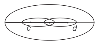
Figure 1. Two curves $c$ and $d$ on $M$

In this work, we study dynamics of the action of Dehn twists $t_{c}$ and $t_{d}$ of ${\rm PMod}(M)\subset{\rm Mod}(M)$ on the Dynnikov coordinate plane. In particular, we find the orbits of the action of Dehn twists $t_{c}$ and $t_{d}$. We note that the dynamics for braid generators on a finitely punctured disc in terms of Dynnikov coordinates was studied in [2], [5].

Theorem 1.1.

The action of each of the Dehn twists $t_{c}$, $t_{d}$, and $t_{e}$ induced on the integer plane $\mathbb{Z}^{2}$ of Dynnikov coordinates $(a,b)$ is piecewise linear and area preserving. The linearity regions, shown in Figure 4 and 5, are bounded by fans of ray, which have similar shape in the domain and the codomain.

A part of formulas used in the proof of this theorem, as well as calculation of some points in Figure 6, are resulted from our work in the project [3], joint with E. Dalyan, E. Medetoğulları, and Ö. Yurttaş, in progress since 2022.

There is an interesting puzzle: to interpret the toric surfaces defined by the fans in Theorem 1.1 and their automorphisms defined due of the similarity of the fans in the domains and codomains.

In a similar context, Ö. Yurttaş, introduced Dynnikov regions to study the dynamics of pseudo-Anosov braids in [12] and informed me that similar regions were considered for any orientable surface in [10] using train tracks.

Our next result is the following theorem.

Theorem 1.2.

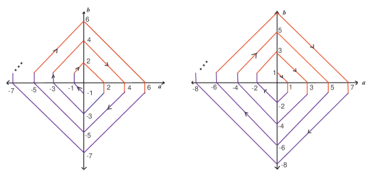
Figure 7. Orbits of the action of $t_{c}t_{d}$ (the blue (resp. red) lines denote the action of $t_{c}$ (resp. $t_{d}$)).

The qualitative dynamics of the action of $t_{c}$, $t_{d}$, and $t_{e}$ on the Dynnikov coordinate plane $\mathbb{Z}^{2}$ is characterized by orbits on Figures 6-7.

Corollary 1.3.

The sequence of values generated by the iteration of $t_{c}$ (resp. $t_{d}$) given by Equation 5 (resp. Equation 6) flows into the second quadrant (resp. the fourth quadrant). The second quadrant is preserved by $t_{c}$ and the fourth quadrant is preserved by $t_{d}.$

We will call these quadrants in Corollary 1.3 black holes.

By using these theorems, we explore some applications which are as follows: Let C denote the set of isotopy classes of essential simple closed curves in $M$. Since the surface $M$ is a thrice-punctured disc, the set C coincides with the curve complex C(M) of $M$, since C(M) is discrete. Using this correspondence, we can encode the curve complex C(M), taking as input their Dynnikov coordinates. Let $\Delta$ be a subset of C(M) consisting of the vertices $v_{c}$, $v_{d}$, and $v_{e}$. These vertices are the isotopy classes of essential simple closed curves $c$, $d$, and $e$ as shown in Figure 2 and the Dynnikov coordinates of $c$, $d$, and $e$ are $(0,1)$, $(0,-1)$, and $(-1,0)$, respectively.

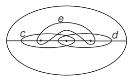
Figure 2.

In Section 4, we describe an algorithm for finding the distance to the set $\Delta$ from an arbitrary vertex in C(M). This algorithm provides a very efficient way to compute how many Dehn twists are used to reach $\Delta$ from a vertex in C(M).

In Section 5, we present a simple proof of the following theorem (cf., [9]).

Theorem 1.4.

The group generated by the Dehn twists $t^{2}_{c}$, $t^{2}_{d}$, and $t^{2}_{e}$ is isomorphic to the free group of rank 3, where $c$, $d$, and $e$ are simple closed curves as in depicted Figure 2.

In connection with this result, S.P. Humphries [7], H. Hamidi-Tehrani [8] and    E. Dalyan, E. Medetog̃ulları, F. Atalan, and Ö. Yurttaş [3] address the question of whether the $n$ Dehn twists generate the free group $F_{n}$ under certain conditions. S. Kolay [9] also investigates what subgroups of the mapping class group of the torus are generated by three uniform powers of Dehn twists.

In Section 6, we give also an algorithm to determine the action of the pseudo-Anosov maps $t_{d}t_{c}^{-1}$ and $t_{d}^{-1}t_{c}$ of $M$ via the orbits of the action of $t_{c}$ and $t_{d}$. This algorithm reveals how the iteration evolves geometrically. We end up with a puzzling task to explain some Diophantine property of the orbits. It may be interesting to compare our results with the ones in [11, Example 4.4], where a similar action is studied for the product of half-twists $\sigma_{c}\sigma_{d}^{-1}$ and its dynamics is also explicitly described in [13, Figure 8] .

Finally, in the appendix, we give a transparent expression of the Dynnikov coordinates in $M$ in terms of $(p,q)$-coordinates on one holed torus via a double branched cover over $M$, which looks new to the best of our knowledge.

Acknowledgements

I would like to thank the Max Planck Institute for Mathematics in Bonn for its hospitality, excellent working conditions, and financial support. I am very grateful to S. Finashin for his valuable geometric comments and suggestions. I would also like to thank Ö. Yurttaş for some references. Finally, the author dedicates this paper to her mother, Z. Atalan, with deep gratitude for her constant moral support throughout its preparation.

2. Preliminaries

Let $f$ be a mapping class which is not the identity. Then, by Thurston’s classification of surface homeomorphisms, one of the following holds:
(1) $f$ is periodic, that is, $f^{n}=1$ for some $n\geq 2$,
(2) $f$ is reducible, i.e. there is a (closed) one-dimensional submanifold $a$ of a surface S such that $f(a)=a$,
(3) $f$ is pseudo-Anosov if and only if $f$ is neither periodic nor reducible.

We note that if we consider $M$ as a sphere with four punctures then the pure mapping class group ${\rm PMod}(M)$ is isomorphic to $F_{2}$. In this case, the elements of ${\rm PMod}(M)$ different from the identity are either reducible or pseudo-Anosov. Moreover, conjugates of nonzero powers of $t_{c}$, $t_{d}$ and $t_{c}t_{d}$ are the only reducible elements in ${\rm PMod}(M)$ (see Lemma 3.4 in [1]).

I.A. Dynnikov introduced a coding for integral laminations on a sphere with $n+3$ punctures in [2].

Let S denote the set of finite unions of pairwise disjoint essential simple closed curves on $n$-punctured disc, up to isotopy. For convenience, we denote the minimum intersection number of $l\in\textit{S}$ with each of the arcs $\alpha_{i}$ and $\beta_{i}$ by the same symbols ($\alpha_{i}$ and $\beta_{i}$ are illustrated in Figure 3 for the case $n=3$). Then there is a bijection $\rho:\textit{S}\to\mathbb{Z}^{2n-4}\setminus\{0\}$ defined by $\rho(l)=(a_{i},b_{i})$ for $l\in\textit{C}$, where

$$a_{i}=\frac{\alpha_{2i}-\alpha_{2i-1}}{2}\,\,\,and\,\,\,b_{i}=\frac{\beta_{i}-\beta_{i+1}}{2}$$

for $1\leq i\leq n-2.$ $\rho$ is called the Dynnikov coordinate function (in fact, the restriction of the Dynnikov coordinate function, see [5] for more details).

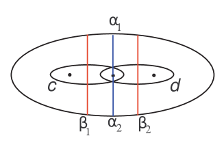
Figure 3. Two curves $c$ and $d$ on $M$

In this work, we consider $M$ as a $3$-punctured disc. The mapping class group ${\rm Mod}(M)$ of $M$ is isomorphic to Artin’s braid group $B_{3}$. It acts on Dynnikov coordinate plane, i.e., $\mathbb{Z}^{2}\setminus\{0\}$ (see [5]). Given $\phi\in B_{3}$, $\psi:\mathbb{Z}^{2}\setminus\{0\}\to\mathbb{Z}^{2}\setminus\{0\}$ is defined by $\psi(a,b)=\rho\circ\phi\circ\rho^{-1}(a,b)$.

The update rules so called describe in [5] the action of the Artin braid generators $\sigma_{1}$ and $\sigma_{2}$ (and their inverses) on $\mathbb{Z}^{2}\setminus\{0\}$. For any $l\in\textit{C}$, with $\rho(l)=(a,b)$, let $\rho(\sigma_{i}(l))=(a^{\prime},b^{\prime})$ for $i=1,2$. By Lemma 4 in [5], we have the following equations:

(1) $$a^{\prime}=a+b-max\{0,a,b\},\,\,\,\,b^{\prime}=max\{b,0\}-a\,\,for\,\,\sigma_{1}\\$$

(2) $$a^{\prime}=max\{a+max\{0,b\},b\},\,\,\,\,b^{\prime}=b-(a+max\{0,b\})\,\,for\,\,\sigma_{2}$$

By Lemma 5 in [5], we have also the following equations:

(3) $$a^{\prime}=max\{0,a+max\{0,b\}\}-b,\,\,\,b^{\prime}=a+max\{0,b\}\,\,for\,\,\sigma_{1}^{-1}$$

(4) $$a^{\prime}=a-max\{a+b,0,b\},\,\,\,b^{\prime}=a+b-max\{0,b\}\,\,for\,\,\sigma_{2}^{-1}$$

3. Dynamics of the actions of ${\rm PMod}(M)$ in Dynnikov coordinate plane $\mathbb{Z}^{2}$

3.1. Proof of Theorem 1.1.

To describe the natural action of ${\rm PMod}(M)$ on $\mathbb{Z}^{2}$ viewed as Dynnikov coordinate plane, we present the action of generators $t_{c}$, $t_{d}\in{\rm PMod}(M)$, where $c$ and $d$ shown in Figure 3 have Dynnikov coordinates $(0,1)$ and $(0,-1)$, respectively.

Since $t_{c}=\sigma_{1}^{2}$ and $t_{d}=\sigma_{2}^{2}$, for any $l\in\textit{C}$ with $\rho(l)=(a,b)\neq(0,0)$, the Equations 1 and 2 give the following Equations 5 and 6, respectively. It is obvious that $t_{e}=(t_{c}t_{d})^{-1}$ and the Dynnikov coordinate of $e$ is $(-1,0)$.

(5) $$\rho(\sigma_{1}^{2}(l))=\rho(t_{c}(l))=\left\{\begin{array}[]{llll}(b-a,-b)&{\rm~if}\;a\geq 0,b\leq a\qquad\ \text{Region A}\\ (b-a,b-2a)&{\rm~if}\;0\leq a\leq b\leq 2a\quad\text{Region B}\\ (a,b-2a)&{\rm~if}\;2a\leq b,b\geq 0\qquad\text{Region C}\\ (a+b,-2a-b)&{\rm~if}\;a\leq 0,b\leq 0\qquad\ \text{Region D}\\ \end{array}\right.$$

(6) $$\rho(\sigma_{2}^{2}(l))=\rho(t_{d}(l))=\left\{\begin{array}[]{ll}(b-a,-b)&{\rm~if}\;a\leq 0,a\leq b\qquad\ \text{Region -A}\\ (b-a,b-2a)&{\rm~if}\;2a\leq b\leq a\leq 0\quad\text{Region -B}\\ (a,b-2a)&{\rm~if}\;b\leq 2a,b\leq 0\qquad\text{Region -C}\\ (a+b,-2a-b)&{\rm~if}\;a\geq 0,b\geq 0\qquad\ \text{Region -D}\\ \end{array}\right.$$

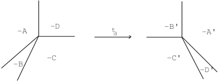
Figure 4.

Figure 4 shows the linearity domains $A-D$ for the action of $t_{c}$ and their images $A^{\prime}-D^{\prime}$. For $t_{d}$ the linearity domains and their images are just opposite. ∎

It turns out that the fan of rays bordering the linearity domains is obtained by rotating the fan for their images by $\frac{\pi}{2}$. To explain it looks like a challenging puzzle.

(7) $$\rho(\sigma_{1}^{2}\sigma_{2}^{2}(l))=\rho(t_{c}t_{d}(l))=\left\{\begin{array}[]{llllll}(-3a+b,2a-b)&{\rm~if}\;a\geq 0,b\leq 0&E^{\prime}\\ (-3a-2b,2a+b)&{\rm~if}\;a\geq 0,b\geq 0&D^{\prime}\\ (a-2b,b)&{\rm~if}\;a\leq 0,\frac{a}{2}\leq b&C^{\prime}\\ (a-2b,2a-3b)&{\rm~if}\;2b\leq a\leq\frac{3b}{2}\leq 0&B^{\prime}\\ (-a+b,2a-3b)&{\rm~if}\;\frac{3b}{2}\leq a\leq b\leq 0&A^{\prime}\\ (-a+b,-b)&{\rm~if}\;b\leq a\leq 0&F^{\prime}\\ \end{array}\right.$$

(8) $$\rho(t_{e}(l))=\rho((t_{c}t_{d})^{-1}(l))=\left\{\begin{array}[]{llllllll}(-3a-b,-2a-b)&{\rm~if}\;a\geq 0,b\geq 0&A\\ (-3a+2b,-2a+b)&{\rm~if}\;a\geq 0,b\leq 0&B\\ (a+2b,b)&{\rm~if}\;a\leq 0,b\leq\frac{-a}{2}&C\\ (a+2b,-2a-3b)&{\rm~if}\;0\leq\frac{-a}{2}\leq b\leq\frac{-2a}{3}&D\\ (-a-b,-2a-3b)&{\rm~if}\;0\leq\frac{-2a}{3}\leq b\leq-a&E\\ (-a-b,-b)&{\rm~if}\;0\leq-a\leq b&F\\ \end{array}\right.$$

The linearity domains $A-F$ for the action of $(t_{c}t_{d})^{-1}$ and their images $A^{\prime}-F^{\prime}$ have the same similarity property.

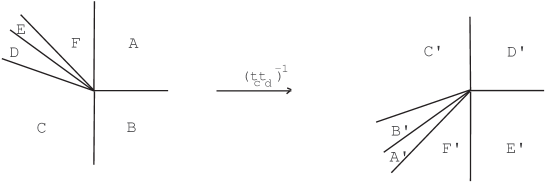
Figure 5.

3.2. Proof of Theorem 1.2.

By Equation 5, the orbit of the action $t_{c}(d)$ is $\{(-1,2k-1),\,\,(1,2k-1)|k\in\mathbb{N}\}$, where $(-1,2k-1)=\rho(t_{c}^{k}(d))$ and $(1,2k-1)=\rho(t_{c}^{-k}(d))$. By Equation 6, the orbit of the action $t_{d}(c)$ is $\{(1,-(2k-1)),\,\,(-1,-(2k-1))|k\in\mathbb{N}\}$, where $(1,-(2k-1))=\rho(t_{d}^{k}(c))$ and $(-1,-(2k-1))=\rho(t_{d}^{-k}(c))$. The orbits of the action of $t_{c}$ and $t_{d}$ on the Dynnikov coordinate plane are as shown in Figure 6.

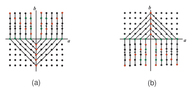
Figure 6. (a) Orbits of the action of $t_{c}$ (b) Orbits of the action of $t_{d}$

Also, we have

$$\rho(\underbrace{t_{c}t_{d}t_{c}t_{d}t_{c}}_{k-times}(d))=(-k,1),$$

$$\rho(\underbrace{t_{d}t_{c}t_{d}t_{c}t_{d}}_{k-times}(c))=(k,-1),$$

$$\rho(\underbrace{t_{c}^{-1}t_{d}^{-1}t_{c}^{-1}t_{d}^{-1}t_{c}^{-1}}_{k-times}(d))=(k,1),$$

$$\rho(\underbrace{t_{d}^{-1}t_{c}^{-1}t_{d}^{-1}t_{c}^{-1}t_{d}^{-1}}_{k-times}(c))=(-k,-1)$$

for some integer $k\geq 1$.

Using Equations 5, 6 and 8 we immediately complete the proof of Theorem 1.2 and Corollary 1.3 as well. ∎

4. The curve complex C(M) via Dynnikov Coordinate Plane

The curve complex C(S) on a surface $S$ is the abstract simplicial complex whose vertices are the isotopy classes of essential simple closed curves. A set of vertices $\{v_{0},v_{1},\ldots,v_{k}\}$ is defined to be a $k$-simplex if and only if $v_{0},v_{1},\ldots,v_{k}$ can be represented by pairwise disjoint curves. Since there is no disjoint essential isotopy classes of simple closed curves in $M$, C(M) is discrete. In this case, C(M) is the set of isotopy classes of simple closed curves C. Since the Dynnikov coordinate function $\rho:\textit{C}\to\mathbb{Z}^{2}$ is injective and $\rho(\textit{C})$ is the set of primitive elements of $\mathbb{Z}^{2}$, we can encode the vertices of C(M) by the Dynnikov coordinates of the isotopy classes of essential simple closed curves in $M$. Let us recall that an element $(m,n)$ of $\mathbb{Z}^{2}\setminus\{0\}$ is primitive if and only if $gcd(m,n)=1$ (see [4]).

Let the vertices $v_{c}$, $v_{d}$, and $v_{e}$ denote the isotopy classes of the curves $c$, $d$, and $e$ depicted in Figure 2, respectively. The vertices $v_{c}$, $v_{d}$, and $v_{e}$ are encoded by the Dynnikov coordinates $(0,1)$, $(0,-1)$, and $(-1,0)$ of $c$, $d$, and $e$; respectively in natural way. Similarly, we can code any vertex of C(M) by the set of primitive elements of $\mathbb{Z}^{2}\setminus\{0\}$ via the Dynnikov coordinates. Let $\Delta=\{v_{c},v_{d},v_{e}\}$.

Let $v$ be any vertex in C(M) with the Dynnikov coordinate $(x,y)$ such that $gcd(x,y)=1$. We want to find the minimum distance between a vertex $v$ and the set $\Delta$. From arbitrary vertex $v$, to reach the vertex $v_{c}$ or $v_{d}$ or $v_{e}$ in $\Delta$, we will use Dehn twists $t_{c}$ and $t_{d}$, and their inverses.

Given a vertex $v$ of C(M) with Dynnikov coordinates $\rho(v)=(x,y)\in\mathbb{Z}^{2}\setminus\{0\}$ the following algorithm finds a mapping class $\phi$ such that $\phi(v)$ reaches the set $\Delta$.

Algorithm of reaching the set $\Delta$

Let $(x,y)\in\mathbb{Z}^{2}\setminus\{0\}$ be the Dynnikov coordinates of $v$ in C(M) with $gcd(x,y)=1$. We will write $(x^{\prime},y^{\prime})\in\mathbb{Z}^{2}\setminus\{0\}$ to denote the Dynnikov coordinates of $\psi(v)$, where $\psi$ is Dehn twist $t_{c}$ or $t_{d}$.

Algorithm. Given a vertex $v$ of C(M) let $\rho(v)=(x,y)\in\mathbb{Z}^{2}\setminus\{0\}$ with $gcd(x,y)=1$.

Step 1: If $y>0$, apply forward $2|x|$ units along $|x|^{th}$ level of orbits of the action of $t_{c}$, let $(x^{\prime},y^{\prime})=\rho(v^{\prime})$, where $v^{\prime}=t_{c}(v)$, if $x>0$ and apply backward $2|x|$ units along $|x|^{th}$ level of orbits of the action of $t_{c}$, let $(x^{\prime},y^{\prime})=\rho(v^{\prime})$, where $v^{\prime}=t_{c}^{-1}(v)$ if $x<0$. If $x^{\prime}=0$, input the pair $(x^{\prime},y^{\prime})$ to Step 3. If $x^{\prime}\neq 0$ and $y^{\prime}>0$, then input the pair $(x^{\prime},y^{\prime})$ to Step 1. If $y^{\prime}=0$ and $x^{\prime}>0$, then input the pair $(x^{\prime},y^{\prime})$ to Step 4. If $y^{\prime}=0$ and $x^{\prime}<0$, then input the pair $(x^{\prime},y^{\prime})$ to Step 5.

Otherwise input the pair $(x^{\prime},y^{\prime})$ to Step 2.

Step 2: If $y<0$, apply backward $2|x|$ units along $|x|^{th}$ level of orbits of the action of $t_{d}$, let $(x^{\prime},y^{\prime})=\rho(v^{\prime})$, where $v^{\prime}=t_{d}^{-1}(v)$ if $x>0$ and apply forward $2|x|$ units along $|x|^{th}$ level of orbits of the action of $t_{d}$, let $(x^{\prime},y^{\prime})=\rho(v^{\prime})$ where $v^{\prime}=t_{d}(v)$ if $x<0$. If $x^{\prime}=0$ input the pair $(x^{\prime},y^{\prime})$ to Step 3. If $x^{\prime}\neq 0$ and $y^{\prime}<0$, then input the pair $(x^{\prime},y^{\prime})$ to Step 2. If $y^{\prime}=0$ and $x^{\prime}>0$, then input the pair $(x^{\prime},y^{\prime})$ to Step 4. If $y^{\prime}=0$ and $x^{\prime}<0$, then input the pair $(x^{\prime},y^{\prime})$ to Step 5.

Otherwise input the pair $(x^{\prime},y^{\prime})$ to Step 1.

Step 3: Since $x=0$, $v_{c}$ is reached if $y>0$, and $v_{d}$ is reached if $y<0$. Write Dehn twists used in Step 1 and Step 2 in order to express the mapping class $\psi$ reaching $v_{c}$ or $v_{d}$.

Step 4: If $y=0$ and $x>0$, apply forward $2|x|$ units along $|x|^{th}$ level of orbits of the action of $t_{c}$, let $(x^{\prime},y^{\prime})=\rho(v^{\prime})$, where $v^{\prime}=t_{c}(v)$ or apply backward $2|x|$ units along $|x|^{th}$ level of orbits of the action of $t_{d}$, let $(x^{\prime},y^{\prime})=\rho(v^{\prime})$, where $v^{\prime}=t_{d}^{-1}(v)$. Then input $(x^{\prime},y^{\prime})$ to Step 5.

Step 5: Since $y=0$ and $x<0$, $v_{e}$ is reached. Write Dehn twists used in Step 1, Step 2, and Step 4 in order to express the mapping class $\psi$ reaching $v_{e}$.

Example 1. Let us take the vertex $v$ in C(M) with the Dynnikov coordinate $(x,y)=(10,3)$. Then, since $y=3>0$ and $x=10>0$, by Step 1, we apply forward $20$ units along $10^{th}$ level of orbits of the action of $t_{c}$, we have $\rho(v^{\prime})=\rho(t_{c}(v))=(-7,-3)$. Since $x<0$, $y<0$, by Step 2, we apply forward $2|x|=2|-7|=14$ units along $7^{th}$ level of orbits of the action of $t_{d}$, we get $\rho(v^{\prime\prime})=\rho(t_{d}(v^{\prime}))=(4,3)$. Since $y=3>0$ and $x=4>0$, by Step 1, we apply forward $8$ units along $4^{th}$ level of orbits of the action of $t_{c}$, we have $\rho(v^{\prime\prime\prime})=\rho(t_{c}(v^{\prime\prime}))=(-1,-3)$. Since $x<0$, $y<0$, by Step 2, we apply forward $2$ units along $1^{st}$ level of orbits of the action of $t_{d}$, we get $\rho(v^{(4)})=\rho(t_{d}(v^{\prime\prime\prime}))=(-1,-1)$. Again, we apply forward $2$ units along $1^{st}$ level of orbits of the action of $t_{d}$, we conclude that $\rho(v^{(5)})=\rho(t_{d}(v^{(4)}))=(0,1)$, we reach the vertex $v_{c}$. Hence, we obtain that

$$(10,3)\stackrel{{\scriptstyle t_{c}}}{{\rightarrow}}(-7,-3)\stackrel{{\scriptstyle t_{d}}}{{\rightarrow}}(4,3)\stackrel{{\scriptstyle t_{c}}}{{\rightarrow}}(-1,-3)\stackrel{{\scriptstyle t_{d}}}{{\rightarrow}}(-1,-1)\stackrel{{\scriptstyle t_{d}}}{{\rightarrow}}(0,1)$$

Example 2. Let us take the vertex $v$ in C(M) with the Dynnikov coordinate $(x,y)=(3,10)$. Then, since $y=10>0$ and $x=3>0$, by Step 1, we apply forward $6$ units along $3^{th}$ level of orbits of the action of $t_{c}$, we have $\rho(v^{\prime})=\rho(t_{c}(v))=(3,4)$. Since $y=4>0$ and $x=3>0$, by Step 1, we apply forward $6$ units along $3^{th}$ level of orbits of the action of $t_{c}$, we have $\rho(v^{\prime\prime})=\rho(t_{c}(v^{\prime}))=(1,-2)$. Since $x=1>0$, $y=-2<0$, apply backward $2$ units along $1^{st}$ level of orbits of the action of $t_{d}$, we have $\rho(v^{\prime\prime\prime})=\rho(t_{d}^{-1}(v^{\prime\prime}))=(1,0)$. By Step 4, $y=0$ and $x=1>0$, we can apply forward $2$ units along $1^{st}$ level of orbits of the action of $t_{c}$, we get $\rho(v^{(4)})=\rho(t_{c}(v^{\prime\prime\prime}))=(-1,0)$, we reach the vertex $v_{e}$. Hence, we have

$$(3,10)\stackrel{{\scriptstyle t_{c}}}{{\rightarrow}}(3,4)\stackrel{{\scriptstyle t_{c}}}{{\rightarrow}}(1,-2)\stackrel{{\scriptstyle t_{d}^{-1}}}{{\rightarrow}}(1,0)\stackrel{{\scriptstyle t_{c}}}{{\rightarrow}}(-1,0)$$

5. Proof of Theorem 1.4

In this section, we consider three isotopy classes of essential simple closed curves with Dynnikov coordinates $(0,1)$, $(0,-1)$, and $(-1,0)$ denoted by $c$, $d$, and $e$, respectively in $M$ as in Figure 2. Then, the group generated by Dehn twists $t_{c}^{2}$, $t_{d}^{2}$, and $t_{e}^{2}$ is isomorphic to the free group of rank $3$, where $t_{e}=(t_{c}t_{d})^{-1}$ is given in Equation 8.

S. Kolay deals with subgroups of the mapping class group of the torus generated by powers of Dehn twists in [9]. S. Kolay also translates his results in the braid group $B_{3}$ (see Section 10 in [9]).

Before proving Theorem 1.4, we recall that the group generated by Dehn twists $t_{c}$ and $t_{d}$ is isomorphic to the free group of rank $2$, see, e.g., [3].

Proof.

Let $G$ be a group generated by Dehn twists $t_{c}^{2}$, $t_{d}^{2}$, and $t_{e}^{2}$. We recall that C is the set of isotopy classes of simple closed curves in $M$. Let $(a_{l},b_{l})$ denote the Dynnikov coordinates of $l\in\textit{C}$. We will use the following the ping pong lemma:

Lemma 5.1.

(Ping pong lemma). Let $G$ be a group acting on a set $X$. Let $g_{1},\ldots,g_{k}$ be elements of $G$. Suppose that there are nonempty, disjoint subsets $X_{1},\ldots,X_{k}$ of $X$ with the property that, for each $i$ and each $j\neq i$, we have $g_{i}^{p}(X_{j})\subset X_{i}$ for every integer $p\neq 0$. Then the group generated by the $g_{m}$ is a free group of rank $k$.

Let us define sets $\textit{C}_{1}$, $\textit{C}_{2}$, and $\textit{C}_{3}$ as follows:
$\textit{C}_{1}=\{l\in\textit{C}\,|\,b_{l}\geq|a_{l}|\,\},\,\,\textit{C}_{2}=\{l\in\textit{C}\,|\,b_{l}\leq-|a_{l}|\,\}$ and $\textit{C}_{3}=\{l\in\textit{C}\,|\,a_{l}<0,\,\,a_{l}<b_{l}<-a_{l}\}$.

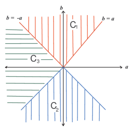
Figure 8. The regions of the sets of $\textit{C}_{1}$, $\textit{C}_{2}$, and $\textit{C}_{3}$

Since the Dynnikov coordinates of the curves $c$, $d$, and $e$ in the Figure 2 are $(0,1)$, $(0,-1)$, and $(-1,0),$ respectively, $a_{c}=0,\,\,b_{c}=1>0$, so, $c\in\textit{C}_{1}$ and $a_{d}=0,\,\,b_{d}=-1<0$, so, $d\in\textit{C}_{2}$. We have also $e\in\textit{C}_{3}$, since $a_{e}=-1,\,\,b_{e}=0$, we have $-2<0<2$. So, $\textit{C}_{1}$, $\textit{C}_{2}$, and $\textit{C}_{3}$ are nonempty, disjoint subsets of C (see Figure 8).

By applying Lemma 5.1, the proof reduces to verifying that $t_{c}^{2p}(\textit{C}_{2}\cup\textit{C}_{3})\subset\textit{C}_{1}$, $t_{d}^{2p}(\textit{C}_{1}\cup\textit{C}_{3})\subset\textit{C}_{2}$, $t_{e}^{2p}(\textit{C}_{1}\cup\textit{C}_{2})\subset\textit{C}_{3}$, for $p\neq 0.$ Because of symmetry, we may assume that $p>0$.

$t_{c}^{2p}(\textit{C}_{2}\cup\textit{C}_{3})\subset\textit{C}_{1}$:

If $l\in\textit{C}_{2}\cup\textit{C}_{3}$, then we have $b_{l}<-a_{l}$ if $a_{l}\leq 0$ and $b_{l}\leq-a_{l}$ if $a_{l}\geq 0$. Then, if $a_{l}\leq 0$, by Equation 5 we have two cases:

Case 1.($b\leq 0$)

$$(a_{l},b_{l})\stackrel{{\scriptstyle t_{c}}}{{\rightarrow}}(a_{l}+b_{l},-2a_{l}-b_{l})\stackrel{{\scriptstyle t_{c}}}{{\rightarrow}}(a_{l}+b_{l},-4a_{l}-3b_{l}).$$

Case 2.($b\geq 0$)

$$(a_{l},b_{l})\stackrel{{\scriptstyle t_{c}}}{{\rightarrow}}(a_{l},-2a_{l}+b_{l})\stackrel{{\scriptstyle t_{c}}}{{\rightarrow}}(a_{l},-4a_{l}+b_{l}).$$

If $a_{l}\geq 0$,

$$(a_{l},b_{l})\stackrel{{\scriptstyle t_{c}}}{{\rightarrow}}(-a_{l}+b_{l},-b_{l})\stackrel{{\scriptstyle t_{c}}}{{\rightarrow}}(-a_{l}+b_{l},2a_{l}-3b_{l}).$$

It is clear that for each image under $t_{c}^{2}$ above the first component is negative and the second component is positive. Then, we obtain that $-4a_{l}-3b_{l}\geq|a_{l}+b_{l}|$ from Case 1, $-4a_{l}+b_{l}\geq|a_{l}|$ from Case 2, and $2a_{l}-3b_{l}\geq|-a_{l}+b_{l}|$ from the case $a_{l}\geq 0$. Hence $t_{c}^{2}(l)=l^{\prime}$ is in $\textit{C}_{1}$.

Now, let us look at the $p$-th iterations of $t_{c}$ of the above cases. If the first component of the Dynnikov coordinate is negative and the second one is positive, by Equation 5, the $p$-th iterate of $t_{c}$ is

(9) $$\rho(t_{c}^{p}(l))=(a_{l},-2pa_{l}+b_{l}),$$

for $p\geq 1$.

Case 1.($b_{l}\leq 0$) By Equation 9, we obtain that $(a_{l}+b_{l},-4a_{l}-3b_{l})\stackrel{{\scriptstyle t_{c}^{2p}}}{{\rightarrow}}(a_{l}+b_{l},-(4p+4)a_{l}-(4p+3)b_{l})$, for $p\geq 1$. Since $b_{l^{\prime}}=-(4p+4)a_{l}-(4p+3)b_{l}\geq|a_{l}+b_{l}|$ and $a_{l}\leq 0$, it follows that $t_{c}^{2p}(l)=l^{\prime}\in\textit{C}_{1}$.

Case 2.($b_{l}\geq 0$) We have $(a_{l},-4a_{l}+b_{l})\stackrel{{\scriptstyle t_{c}^{2p}}}{{\rightarrow}}(a_{l},-(4p+4)a_{l}+b_{l})$, for $p\geq 1$. Since $b_{l^{\prime}}=-4(p+1)a_{l}+b_{l}\geq|a_{l}|$ and $a_{l}\leq 0$, we obtain that $t_{c}^{2p}(l)=l^{\prime}\in\textit{C}_{1}$.

The case $a_{l}\geq 0$. We obtain that $(-a_{l}+b_{l},2a_{l}-3b_{l})\stackrel{{\scriptstyle t_{c}^{2p}}}{{\rightarrow}}(-a_{l}+b_{l},(4p+2)a_{l}-(4p+3)b_{l})$, for $p\geq 1$. Since $b_{l^{\prime}}=(4p+2)a_{l}-(4p+3)b_{l}\geq|-a_{l}+b_{l}|$ and $a_{l}\geq 0$, $b_{l}\leq 0$ we obtain that $t_{c}^{2p}(l)=l^{\prime}\in\textit{C}_{1}$.

$t_{d}^{2p}(\textit{C}_{1}\cup\textit{C}_{3})\subset\textit{C}_{2}$:

If $l\in\textit{C}_{1}\cup\textit{C}_{3}$, then we have $b_{l}>a_{l}$ if $a_{l}\leq 0$ and $b_{l}\geq a_{l}$ if $a_{l}\geq 0$. If $a_{l}\leq 0$, then by Equation 6, we have two cases:

Case 1. ($b_{l}\leq 0$ and $a_{l}<b_{l}<0$).

$$(a_{l},b_{l})\stackrel{{\scriptstyle t_{d}}}{{\rightarrow}}(\underbrace{-a_{l}+b_{l}}_{\geq 0},\underbrace{-b_{l}}_{\geq 0})\stackrel{{\scriptstyle t_{d}}}{{\rightarrow}}(\underbrace{-a_{l}}_{\geq 0},\underbrace{2a_{l}-b_{l}}_{\leq 0}).$$

Case 2. ($b_{l}\geq 0$)

$$(a_{l},b_{l})\stackrel{{\scriptstyle t_{d}}}{{\rightarrow}}(\underbrace{-a_{l}+b_{l}}_{\geq 0},\underbrace{-b_{l}}_{\leq 0})\stackrel{{\scriptstyle t_{d}}}{{\rightarrow}}(\underbrace{-a_{l}+b_{l}}_{\geq 0},\underbrace{2a_{l}-3b_{l}}_{\leq 0}).$$

If $a_{l}\geq 0$, then $b_{l}\geq 0$. In this case, we have

$$(a_{l},b_{l})\stackrel{{\scriptstyle t_{d}}}{{\rightarrow}}(\underbrace{a_{l}+b_{l}}_{\geq 0},\underbrace{-2a_{l}-b_{l}}_{\leq 0})\stackrel{{\scriptstyle t_{d}}}{{\rightarrow}}(\underbrace{a_{l}+b_{l}}_{\geq 0},\underbrace{-4a_{l}-3b_{l}}_{\leq 0}).$$

Since all images under $t_{d}^{2}$ above the first component is positive and the second one is negative. Then, we obtain that $2a_{l}-b_{l}\leq-|a_{l}|$ from Case 1, $2a_{l}-3b_{l}\leq-|-a_{l}+b_{l}|$ from Case 2, and $-4a_{l}-3b_{l}\leq-|a_{l}+b_{l}|$ from the case $a_{l}\geq 0$. Hence $t_{d}^{2}(l)=l^{\prime}$ is in $\textit{C}_{2}$.

If the first component of the Dynnikov coordinate is positive and the second component is negative, by Equation 6, the $p$-th iterate of $t_{d}$ is the same as the formula in Equation 9

(10) $$\rho(t_{d}^{p}(l))=(a_{l},-2pa_{l}+b_{l}),$$

for $p\geq 1$.

Case 1.($b_{l}\leq 0$) By Equation 10, we obtain that $(-a_{l},2a_{l}-b_{l})\stackrel{{\scriptstyle t_{d}^{2p}}}{{\rightarrow}}(-a_{l},(4p+2)a_{l}-b_{l})$, for $p\geq 1$. Since $b_{l^{\prime}}=(4p+2)a_{l}-b_{l}\leq-|a_{l}|$ and $a_{l}\leq 0$, it follows that $t_{d}^{2p}(l)=l^{\prime}\in\textit{C}_{2}$.

Case 2.($b_{l}\geq 0$) We have $(-a_{l}+b_{l},2a_{l}-3b_{l})\stackrel{{\scriptstyle t_{d}^{2p}}}{{\rightarrow}}(-a_{l}+b_{l},(4p+2)a_{l}-(4p+3)b_{l})$, for $p\geq 1$. Since $b_{l^{\prime}}=(4p+2)a_{l}-(4p+3)b_{l}\leq-|-a_{l}+b_{l}|$ and $a_{l}\leq 0$, we obtain that $t_{d}^{2p}(l)=l^{\prime}\in\textit{C}_{2}$.

The case $a_{l}\geq 0$. We obtain that $(a_{l}+b_{l},-4a_{l}-3b_{l})\stackrel{{\scriptstyle t_{d}^{2p}}}{{\rightarrow}}(a_{l}+b_{l},-(4p+4)a_{l}-(4p+3)b_{l})$, for $p\geq 1$. Since $b_{l^{\prime}}=-(4p+4)a_{l}-(4p+3)b_{l}\leq-|a_{l}+b_{l}|$ and $a_{l}\geq 0$, $b_{l}\geq 0$ we obtain that $t_{d}^{2p}(l)=l^{\prime}\in\textit{C}_{2}$.

$t_{e}^{2p}(\textit{C}_{1}\cup\textit{C}_{2})\subset\textit{C}_{3}$:

If $l\in\textit{C}_{1}\cup\textit{C}_{2}$, then we have $b_{l}\geq|a_{l}|$ or $b_{l}\leq-|a_{l}|$. By Equation 8, we have two cases:

Case 1. ($b_{l}\geq|a_{l}|$).

To show that $t_{e}^{2}(\textit{C}_{1})\subset\textit{C}_{3}$, it is sufficient to show that the images of the essential simple closed curves with Dynnikov coordinates $(1,1)$ and $(-1,1)$ under $t_{e}^{2}$ are in the set $\textit{C}_{3}$ since the piecewise linear action of $t_{e}$. By Equation 8, we have

$$(1,1)\stackrel{{\scriptstyle t_{e}}}{{\rightarrow}}(-4,-3)\stackrel{{\scriptstyle t_{e}}}{{\rightarrow}}(-10,-3).$$

Since $a_{l}=-10<0$ and $-10=a_{l}<-3=b_{l}<10=a_{l}$, $t_{e}^{2}(l)=l^{\prime}$ is in $\textit{C}_{3}$, where $l$ and $l^{\prime}$ are essential simple closed curve with $\rho(l)=(1,1)$ and $\rho(l^{\prime})=(-10,-3)$.

$$(-1,1)\stackrel{{\scriptstyle t_{e}}}{{\rightarrow}}(0,-1)\stackrel{{\scriptstyle t_{e}}}{{\rightarrow}}(-2,-1).$$

Since $a_{l}=-2<0$, $-2=a_{l}<-1=b_{l}<2=a_{l}$, $t_{e}^{2}(l)=l^{\prime}$ is in $\textit{C}_{3}$, where $l$ and $l^{\prime}$ are C with $\rho(l)=(-1,1)$ and $\rho(l^{\prime})=(-2,-1)$.

Case 2. ($b_{l}\leq-|a_{l}|$)

To show that $t_{e}^{2}(\textit{C}_{2})\subset\textit{C}_{3}$, it is sufficient to show that the images of the essential simple closed curves with Dynnikov coordinates $(1,-1)$ and $(-1,-1)$ under $t_{e}^{2}$ are in the set $\textit{C}_{3}$. By Equation 7, we have

$$(1,-1)\stackrel{{\scriptstyle t_{e}}}{{\rightarrow}}(-5,-3)\stackrel{{\scriptstyle t_{e}}}{{\rightarrow}}(-11,-3).$$

Since $a_{l}=-11<0$ and $-11=a_{l}<-3=b_{l}<11=a_{l}$, $t_{e}^{2}(l)=l^{\prime}$ is in $\textit{C}_{3}$, where $l$ and $l^{\prime}$ are C with $\rho(l)=(1,-1)$ and $\rho(l^{\prime})=(-11,-3)$.

$$(-1,-1)\stackrel{{\scriptstyle t_{e}}}{{\rightarrow}}(-3,-1)\stackrel{{\scriptstyle t_{e}}}{{\rightarrow}}(-5,-1).$$

Since $a_{l}=-5<0$, $-5=a_{l}<-1=b_{l}<5=a_{l}$, $t_{e}^{2}(l)=l^{\prime}$ is in $\textit{C}_{3}$, where $l$ and $l^{\prime}$ are essential simple closed curves with $\rho(l)=(-1,-1)$ and $\rho(l^{\prime})=(-5,-1)$.

This finishes the proof. ∎

6. The action of pseudo-Anosov map $t_{d}t_{c}^{-1}$ and $t_{d}^{-1}t_{c}$

In this section, we present an algorithm that determines the action of pseudo-Anosov mapping classes $t_{d}t_{c}^{-1}$ and $t_{d}^{-1}t_{c}$ of $M$ making use of orbits of the action $t_{c}$ and $t_{d}$. This algorithm will demonstrate how the iteration changes geometrically.

Let $(a,b)\in\mathbb{Z}^{2}\setminus\{0\}$ be the Dynnikov coordinates of a simple closed curve $l$ in $M$. We will write $(a^{\prime},b^{\prime})\in\mathbb{Z}^{2}\setminus\{0\}$ to denote the Dynnikov coordinates of $\psi(l)$, where $\psi$ is a generator of ${\rm PMod}(M)$.

Main Algorithm for $t_{d}t_{c}^{-1}$. If $b\geq 0$ apply Algorithm 1 otherwise apply Algorithm 2.

Algorithm 1. Let $(a,b)\in\mathbb{Z}^{2}\setminus\{0\}$ be the Dynnikov coordinates of a simple closed curve $l$ in $M$.

Step 1: Apply backward $2|a|$ units along $|a|^{th}$ level of orbits of the action of $t_{c}$, and input the new coordinates $(a^{\prime},b^{\prime})$. If $b^{\prime}>0$ then input the pair $(a^{\prime},b^{\prime})$ to Step 2.

Otherwise input $(a^{\prime},b^{\prime})$ to Step 3.

Step 2: If $b^{\prime}>0$, apply forward $2(|a^{\prime}|+|b^{\prime}|)$ units along $(|a^{\prime}|+|b^{\prime}|)^{th}$ level of orbits of the action of $t_{d}$, and input the new coordinates $(a^{\prime\prime},b^{\prime\prime})$ to Step 4.

Step 3: If $b^{\prime}\leq 0$, apply forward $2|a^{\prime}|$ units along $|a^{\prime}|^{th}$ level of orbits of the action of $t_{d}$, and input the new coordinates $(a^{\prime\prime},b^{\prime\prime})$ to Step 4.

Step 4: Since $(a^{\prime\prime},b^{\prime\prime})$ is the Dynnikov coordinates of $t_{d}(l^{\prime})$, where $l^{\prime}=t_{c}^{-1}(l)$, and $(a^{\prime},b^{\prime})$ is the Dynnikov coordinates of $t_{c}^{-1}(l)$, $(a^{\prime\prime},b^{\prime\prime})$ is the Dynnikov coordinates of $t_{d}t_{c}^{-1}(l)$.

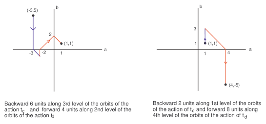
Figure 9.

The following algorithm works for case $b<0$.

Algorithm 2. Let $(a,b)\in\mathbb{Z}^{2}\setminus\{0\}$ be the Dynnikov coordinates of a simple closed curve $l$ in $M$.

Step 1: Apply backward $2(|a|+|b|)$ units along $(|a|+|b|)^{th}$ level of orbits of the action of $t_{c}$, and input the new coordinates $(a^{\prime},b^{\prime})$. If $b^{\prime}>0$ then input the pair $(a^{\prime},b^{\prime})$ to Step 2.

Otherwise input $(a^{\prime},b^{\prime})$ to Step 3.

Step 2: If $b^{\prime}>0$, apply forward $2(|a^{\prime}|+|b^{\prime}|)$ units along $(|a^{\prime}|+|b^{\prime}|)^{th}$ level of orbits of the action of $t_{d}$, and input the new coordinates $(a^{\prime\prime},b^{\prime\prime})$ to Step 4.

Step 3: If $b^{\prime}\leq 0$, apply forward $2|a^{\prime}|$ units along $|a^{\prime}|^{th}$ level of orbits of the action of $t_{d}$, and input the new coordinates $(a^{\prime\prime},b^{\prime\prime})$ to Step 4.

Step 4: Since $(a^{\prime\prime},b^{\prime\prime})$ is the Dynnikov coordinates of $t_{d}(l^{\prime})$, where $l^{\prime}=t_{c}^{-1}(l)$, and $(a^{\prime},b^{\prime})$ is the Dynnikov coordinates of $t_{c}^{-1}(l)$, $(a^{\prime\prime},b^{\prime\prime})$ is the Dynnikov coordinates of $t_{d}t_{c}^{-1}(l)$.

Main Algorithm for $t_{d}^{-1}t_{c}$. If $b\geq 0$ apply Algorithm 1 otherwise apply Algorithm 2.

Algorithm 1. Let $(a,b)\in\mathbb{Z}^{2}\setminus\{0\}$ be the Dynnikov coordinates of a simple closed curve $l$ in $M$.

Step 1: Apply forward $2|a|$ units along $|a|^{th}$ level of orbits of the action of $t_{c}$, and input the new coordinates $(a^{\prime},b^{\prime})$. If $b^{\prime}>0$ then input the pair $(a^{\prime},b^{\prime})$ to Step 2.

Otherwise input $(a^{\prime},b^{\prime})$ to Step 3.

Step 2: If $b^{\prime}>0$, apply backward $2(|a^{\prime}|+|b^{\prime}|)$ units along $(|a^{\prime}|+|b^{\prime}|)^{th}$ level of orbits of the action of $t_{d}$, and input the new coordinates $(a^{\prime\prime},b^{\prime\prime})$ to Step 4.

Step 3: If $b^{\prime}\leq 0$, apply backward $2|a^{\prime}|$ units along $|a^{\prime}|^{th}$ level of orbits of the action of $t_{d}$, and input the new coordinates $(a^{\prime\prime},b^{\prime\prime})$ to Step 4.

Step 4: Since $(a^{\prime\prime},b^{\prime\prime})$ is the Dynnikov coordinates of $t_{d}^{-1}(l^{\prime})$, where $l^{\prime}=t_{c}(l)$, and $(a^{\prime},b^{\prime})$ is the Dynnikov coordinates of $t_{c}(l)$, $(a^{\prime\prime},b^{\prime\prime})$ is the Dynnikov coordinates of $t_{d}^{-1}t_{c}(l)$.

The following algorithm works for case $b<0$.

Algorithm 2. Let $(a,b)\in\mathbb{Z}^{2}\setminus\{0\}$ be the Dynnikov coordinates of a simple closed curve $l$ in $M$.

Step 1: Apply forward $2(|a|+|b|)$ units along $(|a|+|b|)^{th}$ level of orbits of the action of $t_{c}$, and input the new coordinates $(a^{\prime},b^{\prime})$. If $b^{\prime}>0$ then input the pair $(a^{\prime},b^{\prime})$ to Step 2.

Otherwise input $(a^{\prime},b^{\prime})$ to Step 3.

Step 2: If $b^{\prime}>0$, apply backward $2(|a^{\prime}|+|b^{\prime}|)$ units along $(|a^{\prime}|+|b^{\prime}|)^{th}$ level of orbits of the action of $t_{d}$, and input the new coordinates $(a^{\prime\prime},b^{\prime\prime})$ to Step 4.

Step 3: If $b^{\prime}\leq 0$, apply backward $2|a^{\prime}|$ units along $|a^{\prime}|^{th}$ level of orbits of the action of $t_{d}$, and input the new coordinates $(a^{\prime\prime},b^{\prime\prime})$ to Step 4.

Step 4: Since $(a^{\prime\prime},b^{\prime\prime})$ is the Dynnikov coordinates of $t_{d}^{-1}(l^{\prime})$, where $l^{\prime}=t_{c}(l)$, and $(a^{\prime},b^{\prime})$ is the Dynnikov coordinates of $t_{c}(l)$, $(a^{\prime\prime},b^{\prime\prime})$ is the Dynnikov coordinates of $t_{d}^{-1}t_{c}(l)$.

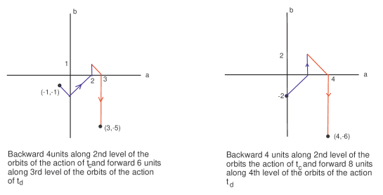
Figure 10.

As an example, we will give the sequences of Dynnikov coordinates for $(t_{d}t_{c}^{-1})^{8}(c)$ and $(t_{d}t_{c}^{-1})^{8}(d)$. We recall that Dynnikov coordinates of $c$ and $d$ are $(0,1)$ and $(0,-1)$, respectively. These values can be calculated via the Dynn.exe program by T. Hall [6].

$$\boxed{\begin{aligned} &(0,1)\stackrel{{\scriptstyle t_{d}t_{c}^{-1}}}{{\rightarrow}}(1,-1)\stackrel{{\scriptstyle t_{d}t_{c}^{-1}}}{{\rightarrow}}(5,-7)\stackrel{{\scriptstyle t_{d}t_{c}^{-1}}}{{\rightarrow}}(29,-41)\stackrel{{\scriptstyle t_{d}t_{c}^{-1}}}{{\rightarrow}}(169,-239)\stackrel{{\scriptstyle t_{d}t_{c}^{-1}}}{{\rightarrow}}\\ &(985,-1393)\stackrel{{\scriptstyle t_{d}t_{c}^{-1}}}{{\rightarrow}}(5741,-8119)\stackrel{{\scriptstyle t_{d}t_{c}^{-1}}}{{\rightarrow}}(33461,-47321)\stackrel{{\scriptstyle t_{d}t_{c}^{-1}}}{{\rightarrow}}(195025,-275807)\end{aligned}}$$

$$\boxed{\begin{aligned} &(0,-1)\stackrel{{\scriptstyle t_{d}t_{c}^{-1}}}{{\rightarrow}}(2,-3)\stackrel{{\scriptstyle t_{d}t_{c}^{-1}}}{{\rightarrow}}(12,-17)\stackrel{{\scriptstyle t_{d}t_{c}^{-1}}}{{\rightarrow}}(70,-99)\stackrel{{\scriptstyle t_{d}t_{c}^{-1}}}{{\rightarrow}}(408,-577)\stackrel{{\scriptstyle t_{d}t_{c}^{-1}}}{{\rightarrow}}\\ &(2378,-3363)\stackrel{{\scriptstyle t_{d}t_{c}^{-1}}}{{\rightarrow}}(13860,-19601)\stackrel{{\scriptstyle t_{d}t_{c}^{-1}}}{{\rightarrow}}(80782,-114243)\stackrel{{\scriptstyle t_{d}t_{c}^{-1}}}{{\rightarrow}}(470832,-665857)\end{aligned}}$$

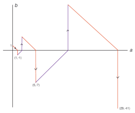
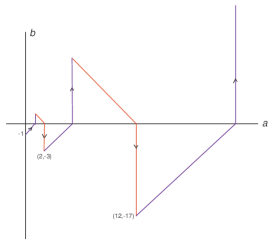
Figure 11. Iterations of $t_{d}t_{c}^{-1}$ applied to $c$ (on the left) and $d$ (on the right)

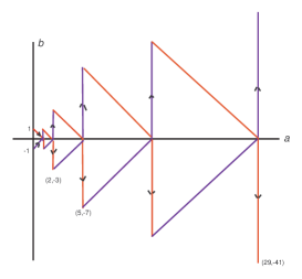
Figure 12.

Remark 6.1.

If the pairs in the sequence generated by iterating $t_{d}t_{c}^{-1}(c)$ are combined with the pairs in the sequence generated by iterating $t_{d}t_{c}^{-1}(d)$ (see Figure 11), respectively; we obtain a sequence of isosceles triangles as shown in Figure 12. The areas of these triangles are 1, 1, 9, 49, 289, etc.

Remark 6.2.

The pairs in the sequence of values generated by the iteration of $t_{d}t_{c}^{-1}(c)$ satisfy the equation $2a^{2}-b^{2}=1$. We can see that the integers $b$ correspond to the integers $m$ in the NSW numbers (named after Newman, Shanks, and Williams) that solve the Diophantine equation $2n^{2}=m^{2}+1$. When the starting point changes, it is observed that the pairs in the sequence generated by iterating $t_{d}t_{c}^{-1}$ satisfy the equation $2a^{2}-b^{2}=Det(A)$, where $A=\left[\begin{array}[]{rr}2a&b\\ b&a\end{array}\right]$.

Appendix. The Dynnikov coordinates in $M$ in terms of $(p,q)$-coordinates on one holed torus via a double branched cover

We consider the double branched cover of a disc $M$ with three punctures which is the one-holed torus $T$, $\pi:T\to M$ (punctures are the branch points). Our model is a flat torus with a hole containing four arcs, as shown in Figure 13. Here, half twists about arcs in the mapping class group of $M$ correspond to Dehn twists about lift of that arc in the mapping class group of $T$, and this induces an isomorphism ${\rm Mod}(T)\cong{\rm Mod}(M)\cong B_{3}$. This isomorphism motivates the use of Dynnikov coordinates. We also note that the mapping class group of the torus is obtained by capping the hole.

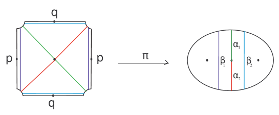
Figure 13.

Let $\gamma$ and $\delta$ be two essential simple closed curves on $T$ intersecting each other at one point. We associate $\gamma$ with the $(1,0)$-coordinate and $\delta$ with the $(0,1)$-coordinate. The projections of $\gamma$ and $\delta$ are $c$ and $d$, respectively, where $c$ and $d$ are as shown in Figure 1. We recall that their Dynnikov coordinates are $(0,1)$ and $(0,-1)$, respectively. Given a $(p,q)$-coordinates in the torus, we can find its Dynnikov coordinates using the formula below:

$$a=\frac{\alpha_{2}-\alpha_{1}}{2}=\frac{|p-q|-|p+q|}{2},$$

$$b=\frac{\beta_{1}-\beta_{2}}{2}=\frac{2|p|-2|q|}{2}=|p|-|q|.$$

References

- [1] F. Atalan and M. Korkmaz, Number of pseudo–Anosov elements in the mapping class group of a four–holed sphere, Turk J. Math., 34 (2010) 585-592.
- [2] I.A. Dynnikov, On a Yang-Baxter mapping and the Dehornoy ordering, Russian Mathematical Surveys, 57(3) (2002) 592-594.
- [3] E. Dalyan, E. Medetog̃ulları, F. Atalan, and S.Ö. Yurttaş, Detecting free products generated by Dehn twists on punctured disks, preprint.
- [4] B. Farb and D. Margalit, A primer on mapping class groups Princeton University Press, New Jersey, 2012.
- [5] T. Hall and S.Ö. Yurttaş, On the topological entropy of families of braids, Topology and its Applications, 156 (2009) 1554–1564.
- [6] T. Hall, Dynn: a program for working with Dynnikov coordinates https:// pcwww.liv.ac.uk/ maths/ tobyhall/ software/.
- [7] S. P. Humphries, Free products in mapping class groups generated by Dehn twists, Glasgow Mathematical Journal, 31(02) (1989) 213-218.
- [8] H. Hamidi-Tehrani, Groups generated by positive multi-twists and the fake lantern problem, Algebr. Geom. Topol., 2:1155–1178, 2002.
- [9] S. Kolay, Subgroups of the mapping class group of the torus generated by powers of Dehn twists, arXiv:1909.07360, 2019.
- [10] D. Margalit, B. Strenner, S. J. Taylor, and S.Ö. Yurttaş, Quadratic-time computations for pseudo-anosov mapping classes, arXiv: 2408.07596v1, 2024.
- [11] S. Ö. Yurttaş, Dynnikov coordinates and pseudo-Anosov braids, Ph.D. thesis, University of Liverpool, 2011.
- [12] S. Ö. Yurttaş, Dynnikov and train track transition matrices of pseudo-anosov braids, Discrete and Continuous Dynamical Systems 36(1) (2016) 541-570.
- [13] S. Ö. Yurttaş, Applications of the Dynnikov coordinate system on the boundary of Teichmüller space, arXiv: 1812.11769v1, 2018.