Mean-field behavior of the quantum Ising susceptibility
and a new lace expansion for the classical Ising model

Abstract

The transverse-field Ising model is widely studied as one of the simplest quantum spin systems. It is known that this model exhibits a phase transition at the critical inverse temperature $\beta_{\mathrm{c}}(q)$, where $q$ is the strength of the transverse field. Björnberg [7] investigated the divergence rate of the susceptibility for the nearest-neighbor model as the critical point is approached by simultaneously changing $q$ and the spin-spin coupling $J$ in a proper manner, with fixed temperature. In this paper, we prove that the susceptibility diverges as $(\beta_{\mathrm{c}}(q)-\beta)^{-1}$ as $\beta\uparrow\beta_{\mathrm{c}}(q)$ for $d>4$ assuming an infrared bound on the space-time two-point function. One of the key elements is a stochastic-geometric representation in Björnberg & Grimmett [6] and Crawford & Ioffe [11]. As a byproduct, we derive a new lace expansion for the classical Ising model (i.e., $q=0$).

1 Introduction and the main results

1.1 Introduction

The Ising model is one of the most-studied models of ferromagnetism. It was invented by Wilhelm Lenz in 1920 [23], but is named after Ernst Ising who proved absence of a phase transition on a 1-dimensional lattice [20]. It is formally defined by the infinite-volume limit of the finite-volume Gibbs distribution $\propto\mathord{\mathrm{e}}^{-\beta\mathcal{H}(\vv{\sigma})}$, where $\beta$ represents the inverse temperature and $\mathcal{H}(\vv{\sigma})$ represents the energy function, called Hamiltonian, for a spin configuration $\vv{\sigma}=\{\sigma_{x}\}_{x\in\Lambda}\in\{\pm 1\}^{\Lambda}$ on a finite graph $(\Lambda,\mathbb{J}_{\Lambda})$:

$$\mathcal{H}_{\Lambda}(\vv{\sigma})=-\sum_{\{x,y\}\in\mathbb{J}_{\Lambda}}J_{x,y}\,\sigma_{x}\,\sigma_{y}.$$ (1.1)

Unless otherwise stated, we assume all spin-spin couplings $J_{x,y}$ are positive (i.e., ferromagnetic).

It is well-known that the Ising model exhibits a sharp phase transition on locally-finite transitive graphs in dimensions $d\geq 2$ [3, 12]: there is a critical point $\beta_{\mathrm{c}}\in(0,\infty)$ such that the susceptibility $\chi_{\beta}$, which is the sum of the infinite-volume limit $\Lambda\uparrow\mathbb{Z}^{d}$ of the two-spin expectation, becomes finite as soon as $\beta<\beta_{\mathrm{c}}$, while the spontaneous magnetization $m_{\beta}$, which is the infinite-volume limit of the single-spin expectation under the plus-boundary condition (i.e., all spins outside of $\Lambda$ are fixed at $+1$), becomes positive as soon as $\beta>\beta_{\mathrm{c}}$. Moreover, it is generally believed that these order parameters exhibit power-law behavior in the vicinity of the critical point, e.g., $\chi_{\beta}\asymp(\beta_{\mathrm{c}}-\beta)^{-\gamma}$ as $\beta\uparrow\beta_{\mathrm{c}}$. The critical exponents, such as $\gamma$, are believed to be universal in the sense that they depend only on the symmetry and the dimension $d$ of the underlying lattice, but not on the microscopic details of the concerned models. For models, such as the nearest-neighbor model on $\mathbb{Z}^{d}$, that satisfy a stronger symmetry condition, called reflection positivity, it is known that $\gamma=1$ in dimensions above the upper critical dimension $d_{\mathrm{c}}=4$; other critical exponents also take on their mean-field values in dimensions $d>d_{\mathrm{c}}$. In two dimensions, on the other hand, Fisher’s scaling or the exact results on the infinite-volume critical two-spin expectation by Wu, McCoy, Tracy and Barouch [36] implies $\gamma=7/4$. In three dimensions, only numerical results are available so far, although there are some interesting predictions from the so-called conformal bootstrap by El-Showk, Paulos, Poland, Rychkov, Simmons-Duffin and Vichi [34].

One of the key elements to show the aforementioned mean-field behavior is an infrared bound on the two-point function, which is a bound in the infrared regime in terms of the underlying random walk generated by the step-distribution $\propto J_{o,x}$. It was first proven for the nearest-neighbor model [14], and then extended to a wider class of models that satisfy reflection positivity [13]. For a more detailed review, see also [5]. It is used to verify the so-called bubble condition, which is a sufficient condition for the mean-field behavior [2, 1, 4] and is the square summability of the two-point function up to the critical point. Although the class of reflection-positive models is large enough to include the nearest-neighbor model, it does not necessarily cover all important models, such as the next-nearest-neighbor models with relatively equal weight and the uniformly spread-out models over the support.

Another way to prove an infrared bound is the lace expansion. It has been successful in various models, such as self-avoiding walk [10, 18], oriented/unoriented percolation [16, 29], lattice trees and lattice animals [17], the contact process [30], the Ising model [31], the $\varphi^{4}$ model [32, 9], the random-connection model [19] and self-repellent Brownian bridges [8]. Since the lace expansion yields a renewal equation for the two-point function, the infrared asymptotics at the critical point can be derived by deconvolution [25], without assuming reflection positivity. However, because of its perturbative nature from the underlying random walk, the dimension $d$ must usually be way higher than the critical dimension $d_{\mathrm{c}}$.

In this paper, we investigate the quantum Ising model under transverse field [24], which is a toy model for quantum spin systems. It has also become popular in the field of computer science, due to its application to combinatorial optimization problems using quantum annealing (e.g., [26, 27, 28]). The model is defined by replacing each spin $\sigma_{x}$ in the classical Hamiltonian $\mathcal{H}_{\Lambda}(\vv{\sigma})$ in (1.1) with $S^{\scriptscriptstyle(3)}_{x}$, which is a tensor product of the z-axis Pauli matrix, and perturbing the Hamiltonian by the transverse field $-q\sum_{x\in\Lambda}S^{\scriptscriptstyle(1)}_{x}$ in the x-axis direction. Since $S^{\scriptscriptstyle(1)}$ and $S^{\scriptscriptstyle(3)}$ do not commute, the model becomes unstable as long as $q>0$, which may increase the value of the critical point $\beta_{\mathrm{c}}(q)$; existence of a phase transition for the transverse-field Ising model and other quantum models (e.g., anisotropic Heisenberg models) was first proved by Ginibre [15]. We are interested in the rate of divergence of the susceptibility $\chi$ as $\beta\uparrow\beta_{\mathrm{c}}(q)$ and finding out how it is affected by quantum effects.

In [7], Björnberg investigated the quantum Ising susceptibility $\chi$ with the nearest-neighbor spin-spin coupling $J_{x,y}=J\mathbbm{1}{\raisebox{-2.0pt}{$\scriptstyle\{\|y-x\|_{1}=1\}$}}$. Since $\chi$ is increasing in $J$ when $\beta$ and $q$ are fixed, there must be a critical point $J_{\mathrm{c}}(q)$ such that $\chi$ converges if $J<J_{\mathrm{c}}(q)$ and diverges if $J>J_{\mathrm{c}}(q)$. He showed that, if $\beta>0$ is fixed and $(J,q)$ approaches $(J_{\mathrm{c}}(q_{0}),q_{0})$ within a certain region, then $\chi$ diverges as $\|(J,q)-(J_{\mathrm{c}}(q_{0}),q_{0})\|_{2}^{-1}$ for $d>4$ (cf., Section 1.3). This appears as if it shows the mean-field behavior $\gamma=1$, but in fact it does not, since the region mentioned above does not cover the ray $\beta\uparrow\beta_{\mathrm{c}}(q)$ with $J$ and $q$ fixed (cf., Figure 1). The restriction to the nearest-neighbor model for $d>4$ is for the use of reflection positivity (so that the two-point function obeys an infrared bound) and a quantum version of the bubble condition.

We show that $\chi$ for the nearest-neighbor model in dimensions $d>4$ indeed exhibits the mean-field behavior $\gamma=1$ as $\beta\uparrow\beta_{\mathrm{c}}(q)$ with $J$ and $q~(\ll 1)$ fixed. This implies that the critical behavior is robust against small quantum perturbation, as long as $d>4$. The proof is based on an inequality for $\partialderivative{\chi}/{\beta}$ that is valid for a wider class of models than that of reflection-positive models. The inequality for $\partialderivative{\chi}/{\beta}$ is obtained by reorganizing two differential inequlities in Björnberg [7]. Those differential inequlities were obtained by using a stochastic-geometric representation in space-time [6, 11]. By setting $q=0$ in this representation, we also derive a new lace expansion for the classical Ising model. In the sequel [21], we will extend the lace expansion to the $q>0$ case, in order to prove the aforementioned mean-field results without assuming reflection positivity.

1.2 Transverse-field Ising model

For each pair of sites $b=\{x,y\}\subset\mathbb{Z}^{d}$, we denote its translation-invariant spin-spin coupling by

$$J_{b}=J_{x,y}=J_{y-x}.$$ (1.2)

For a finite subset $\Lambda\subset\mathbb{Z}^{d}$ containing the origin $o=(0,\dots,0)$, we define its bond set by

$$\mathbb{J}_{\Lambda}=\big{\{}b=\{x,y\}\subset\Lambda\nonscript:\allowbreak\nonscript\mathopen{}J_{b}\neq 0\big{\}}.$$ (1.3)

Throughout this paper, we assume that the spin-spin coupling satisfies the following conditions:

Assumption 1.1.

1. $\mathbb{Z}^{d}$-symmetric: $J_{x}=J_{T(x)}$, where $T(x)$ is the mirror reflection of $x$ with respect to a coordinate hyperplane, or the image of $x$ rotated by 90 degrees around the origin. In addition, $J_{o}=0$.

2. (Strongly) summable: $\exists\alpha>2$ such that $\sum_{x\in\mathbb{Z}^{d}}\lvert x\rvert^{\alpha}J_{x}<\infty$.

3. Irreducible: $\forall x,y\in\mathbb{Z}^{d}$, $\exists v_{1},v_{2},\dots,v_{n}\in\mathbb{Z}^{d}$ such that $J_{x,v_{1}}J_{v_{1},v_{2}}\cdots J_{v_{n},y}>0$.

4. Ferromagnetic: $J_{x}>0$ for every $\{o,x\}\in\mathbb{J}_{\Lambda}$.

We note that the nearest-neighbor model, defined by

$$J_{x}=\begin{cases}J&\text{if }\|x\|_{1}=1,\\ 0&\text{otherwise},\end{cases}$$ (1.4)

where $\|\cdot\|_{p}$ for $p\geq 1$ is the $\ell^{p}$ norm, satisfies the above assumptions.

Next we define the Hamiltonian $H_{\Lambda}$ as an operator acting on $\bigotimes_{x\in\Lambda}\mathbb{C}^{2}=(\mathbb{C}^{2})^{\otimes\Lambda}$ as follows. Let

$$I=\begin{bmatrix}1&0\\ 0&1\end{bmatrix}, S^{\scriptscriptstyle(1)}=\begin{bmatrix}0&1\\ 1&0\end{bmatrix}, S^{\scriptscriptstyle(3)}=\begin{bmatrix}1&0\\ 0&-1\end{bmatrix},$$ (1.5)

and define

$$H_{\Lambda} =H_{\Lambda,0}+Q_{\Lambda}, H_{\Lambda,0} =-\sum_{\{x,y\}\in\mathbb{J}_{\Lambda}}J_{x,y}S_{x}^{\scriptscriptstyle(3)}S_{y}^{\scriptscriptstyle(3)}, Q_{\Lambda} =-q\sum_{x\in\Lambda}S_{x}^{\scriptscriptstyle(1)},$$ (1.6)

where $q\geq 0$ is the strength of the transverse field, and the subscript $x$ in $S^{\scriptscriptstyle(j)}_{x}$ is the location of $S^{\scriptscriptstyle(j)}$ in a tensor product of operators:

$$S^{\scriptscriptstyle(j)}_{x} =\underbrace{I\cdots\otimes I\otimes\underset{\begin{subarray}{c}\uparrow\\ x\end{subarray}}{S^{\scriptscriptstyle(j)}}\otimes I\otimes\cdots I}_{\Lambda}.$$ (1.7)

We use the bra-ket notation commonly used in physics to denote the eigenvectors of $S^{\scriptscriptstyle(3)}$ by

$$\bra{+1}=\begin{bmatrix}1&0\end{bmatrix}, \ket{+1}=\begin{bmatrix}1\\ 0\end{bmatrix}, \bra{-1}=\begin{bmatrix}0&1\end{bmatrix}, \ket{-1}=\begin{bmatrix}0\\ 1\end{bmatrix}.$$ (1.8)

For $\vv{\sigma}=\{\sigma_{x}\}_{x\in\Lambda}$, we define

$$\ket{\vv{\sigma}}=\bigotimes_{x\in\Lambda}\ket{\sigma_{x}},$$ (1.9)

and denote its transpose by $\bra{\vv{\sigma}}$.

Finally we define the expectation at the inverse temperature $\beta\geq 0$ of an operator $A$ on $(\mathbb{C}^{2})^{\otimes\Lambda}$ as

$$\langle A\rangle_{\Lambda}=\frac{\operatorname{Tr}[A\mathord{\mathrm{e}}^{-\beta H_{\Lambda}}]}{\operatorname{Tr}[\mathord{\mathrm{e}}^{-\beta H_{\Lambda}}]}, \operatorname{Tr}[\cdots]=\sum_{\vv{\sigma}\in\{\pm 1\}^{\Lambda}}\innerproduct{[}{[}3]{\vv{\sigma}}{\cdots}{\vv{\sigma}}.$$ (1.10)

In particular, we are interested in the susceptibility defined as

$$\chi_{\Lambda}=\chi_{\Lambda}(\beta,q)=\int_{\mathbb{T}}\odif{t}\sum_{x\in\Lambda}\left\langle S_{o}^{\scriptscriptstyle(3)}(0)S_{x}^{\scriptscriptstyle(3)}(t)\right\rangle_{\Lambda}$$

where $\mathbb{T}$ is the unit torus (i.e., $\interval{0}{1}$ with the periodic-boundary condition) and

$$S_{x}^{\scriptscriptstyle(3)}(t)=\mathord{\mathrm{e}}^{-t\beta H_{\Lambda}}S_{x}^{\scriptscriptstyle(3)}\mathord{\mathrm{e}}^{t\beta H_{\Lambda}}$$ (1.11)

is interpreted in physics as an imaginary-time evolution operator. Since $S^{\scriptscriptstyle(3)}_{x}$ and $H_{\Lambda,0}$ commute, we have that, for any $t\in\mathbb{T}$,

$$\operatorname{Tr}[S_{o}^{\scriptscriptstyle(3)}(0)S_{x}^{\scriptscriptstyle(3)}(t)\mathord{\mathrm{e}}^{-\beta H_{\Lambda,0}}]=\sum_{\vv{\sigma}\in\{\pm 1\}^{\Lambda}}\sigma_{o}\sigma_{x}\mathord{\mathrm{e}}^{-\beta\mathcal{H}_{\Lambda}(\vv{\sigma})}\underbrace{\innerproduct{\vv{\sigma}}{\vv{\sigma}}}_{=1},$$ (1.12)

where $\mathcal{H}_{\Lambda}(\vv{\sigma})$ is the classical Ising Hamiltonian (1.1), hence

$$\chi_{\Lambda}(\beta,0)=\int_{\mathbb{T}}\odif{t}\sum_{x\in\Lambda}\left\langle S_{o}^{\scriptscriptstyle(3)}(0)S_{x}^{\scriptscriptstyle(3)}(t)\right\rangle_{\Lambda}=\sum_{x\in\Lambda}\frac{\sum_{\vv{\sigma}}\sigma_{o}\sigma_{x}\mathord{\mathrm{e}}^{-\beta\mathcal{H}_{\Lambda}(\vv{\sigma})}}{\sum_{\vv{\sigma}}\mathord{\mathrm{e}}^{-\beta\mathcal{H}_{\Lambda}(\vv{\sigma})}}.$$ (1.13)

Since this is identical to the susceptibility for the classical Ising model, $\chi_{\Lambda}$ in (1.2) is a natural extension to the transverse-field Ising model.

1.3 Main results

For now, let us restrict ourselves to the nearest-neighbor model (1.4). Although $\chi_{\Lambda}$ is not increasing in $\beta$ in general due to the quantum effect, it is increasing in $J$, so there is a critical value $J_{\mathrm{c}}=J_{\mathrm{c}}(q)$ such that the infinite-volume limit $\chi=\chi(\beta,q)\equiv\lim_{\Lambda\uparrow\mathbb{Z}^{d}}\chi_{\Lambda}$ is finite as long as $J<J_{\mathrm{c}}$:

$$J_{\mathrm{c}}(q)=\inf\left\{J\geq 0\nonscript:\allowbreak\nonscript\mathopen{}\chi(\beta,q)=\infty\right\}.$$ (1.14)

For $d>4$ with $\beta>0$ fixed, Björnberg [7, Theorem 1.3] proved that $\chi$ exhibits the following mean-field behavior as $(J,q)$ approaches the critical point $(J_{\mathrm{c}}(q_{0}),q_{0})$ along any ray strictly inside the region $\{(J,q):q>q_{0},~0\leq J<J_{\mathrm{c}}(q_{0})\}$ (cf., Figure 1):

$$\chi(\beta,q)\asymp\left\lVert(J,q)-\bigl{(}J_{\mathrm{c}}(q_{0}),q_{0}\bigr{)}\right\rVert_{2}^{-1},$$ (1.15)

where "$\asymp$" means that the ratio of the left-hand side to the right-hand side is bounded away from zero and infinity in the prescribed limit.

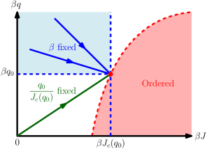
Figure 1: A phase diagram in the $(\beta J,\beta q)$ plane, with the imaginary critical curve (slashed in red). Björnberg [7, Theorem 1.3] covers the blue-shaded region with fixed $\beta$, while Theorem 1.2 covers rays coming out of the origin (e.g., the depicted one in green).

However, this is a bit unsatisfactory from a physics point of view, since it does not cover the limit $q\downarrow q_{0}$ with $J=J_{\mathrm{c}}(q_{0})$ fixed (unlike the temperature, $J$ is usually uncontrollable, as it is inherent in the concerned material). It also does not cover the limit $\beta\uparrow\beta_{\mathrm{c}}(q)$ along the ray $\{(\beta J,\beta q):0\leq\beta<\beta_{\mathrm{c}}(q)\}$ with $J$ and $q$ fixed (cf., Figure 1), where

$$\beta_{\mathrm{c}}(q)=\inf\left\{\beta\geq 0\nonscript:\allowbreak\nonscript\mathopen{}\chi(\beta,q)=\infty\right\}.$$ (1.16)

The following theorem elucidates the behavior of $\chi$ for $d>4$ in the latter region.

Theorem 1.2 (Mean-field behavior of the quantum susceptibility).

For the nearest-neighbor model on $\mathbb{Z}^{d>4}$ with $J>0$ fixed, there are $q_{0}>0$ and $\beta_{0}<\beta_{\mathrm{c}}(q)$ such that, for any $q\in\interval{0}{q_{0}}$, $\chi$ is increasing in $\beta\in[\beta_{0},\beta_{\mathrm{c}}(q))$ and diverges as $\chi\asymp(\beta_{\mathrm{c}}(q)-\beta)^{-1}$ as $\beta\uparrow\beta_{\mathrm{c}}(q)$.

The restriction to the nearest-neighbor model in the above theorem is inherited from the result of Björnberg [7], where he proved an infrared bound only for the nearest-neighbor model, though it is believed to be true for all reflection-positive models that satisfy Assumption 1.1.

The proof of the above theorem is based on a differential inequality for $\chi$ that involves a space-time bubble diagram. The infrared bound mentioned above is used to show convergence of this space-time bubble diagram as long as $d>4$.

To prove the aforementioned differential inequality for $\chi$, we use a stochastic-geometric representation for the transverse-field Ising model. As a byproduct of this representation, we derive the following new lace expansion for the classical Ising model, in which we use the notation

$$\bm{x}=(t_{\bm{x}},x)\in\mathbb{T}\times\Lambda, G(\bm{o},\bm{x})=\langle S^{\scriptscriptstyle(3)}_{o}(0)S^{\scriptscriptstyle(3)}_{x}(t_{\bm{x}})\rangle_{\Lambda}.$$ (1.17)

Here, $\Lambda$ can be any finite set, with any boundary condition (e.g., a torus of side length $2L$).

Theorem 1.3 (The lace expansion for $q=0$).

There are model-dependent expansion coefficients $\pi^{\scriptscriptstyle(j)}\colon(\mathbb{T}\times\Lambda)^{2}\to[0,\infty)$ for $j\geq 0$ such that

$$G(\bm{o},\bm{x})=\pi^{\scriptscriptstyle(\leq j)}(\bm{o},\bm{x})+\int_{\mathbb{T}}\mathrm{d}t\sum_{\begin{subarray}{c}\bm{y},\bm{z}\in\mathbb{T}\times\Lambda:\\ t_{\bm{y}}=t_{\bm{z}}=t\end{subarray}}\beta J_{y,z}\,\pi^{\scriptscriptstyle(\leq j)}(\bm{o},\bm{y})\,G(\bm{z},\bm{x})+(-1)^{j+1}R^{\scriptscriptstyle(j+1)}(\bm{o},\bm{x}),$$ (1.18)

where $\pi^{\scriptscriptstyle(\leq j)}(\bm{o},\bm{x})=\sum_{i=0}^{j}(-1)^{i}\pi^{\scriptscriptstyle(i)}(\bm{o},\bm{x})$. Moreover, the remainder $R^{\scriptscriptstyle(j+1)}(\bm{o},\bm{x})$ is bounded as

$$0\leq R^{\scriptscriptstyle(j+1)}(\bm{o},\bm{x})\leq\int_{\mathbb{T}}\mathrm{d}t\sum_{\begin{subarray}{c}\bm{y},\bm{z}\in\mathbb{T}\times\Lambda:\\ t_{\bm{y}}=t_{\bm{z}}=t\end{subarray}}\beta J_{y,z}\,\pi^{\scriptscriptstyle(j)}(\bm{o},\bm{y})\,G(\bm{z},\bm{x}).$$ (1.19)

Another lace expansion for the classical Ising model [31, 33] was obtained in a totally different way, based on the so-called random-current representation on the lattice (i.e., no time variable). As is roughly explained in the beginning of Section 5, the lace expansion yields an infrared bound on $G$ in a relatively easy way, without assuming reflection positivity. In the sequel [21], we will report on the extension to the $q>0$ case.

1.4 Organization

The remainder of the paper is organized as follows. In Section 2, we prove Theorem 1.2 by using a differential inequality for $\partialderivative{\chi_{\Lambda}}/{\beta}$ (cf., Proposition 2.3) that is a result of two differential inequlities for $\partialderivative{\chi_{\Lambda}}/{J_{b}}$ and $\partialderivative{\chi_{\Lambda}}/{q}$ (cf., Lemma 2.4). In Section 3, we review the stochastic-geometric representation for the transverse-field Ising model [6, 11]. One of the key features of this representation is the so-called source switching (cf., Lemma 3.2). In Section 4, we use this representation and the source switching to explain the aforementioned differential inequalities. Finally, in Section 5, we prove Theorem 1.3 in a heuristic way and give a precise definition of the expansion coefficients $\pi^{\scriptscriptstyle(j)}(\bm{o},\bm{x})$ for $j\geq 0$. Also, we show a diagrammatic bound on $\pi^{\scriptscriptstyle(0)}(\bm{o},\bm{x})$ and briefly explain how to bound the other expansion coefficients.

2 Mean-field behavior of the quantum Ising susceptibility

In this section, we prove Theorem 1.2 by using a differential inequality for the susceptibility (cf., Proposition 2.4), which is a result of combining two differential inequalities in Björnberg [7]. The differential inequality for the susceptibility involves the so-called bubble diagram (cf., (2.2)), whose convergence for $d>4$ is ensured by an infrared bound on the two-point function (cf., Lemma 2.1).

In Section 4, we will explain the derivation of those differential inequalities in Björnberg [7] by using expressions for the derivatives of the susceptibility in Section 2.2 and a stochastic-geometric representation in Section 3.

2.1 Proof of the mean-field behavior of the susceptibility

Let $\Lambda=[-L,L]^{d}\cap\mathbb{Z}^{d}$ be a torus. For $k\in\frac{\pi}{L}\Lambda$ and $\omega\in 2\pi\mathbb{Z}$, we define

$$\hat{J}(k)=\sum_{x\in\mathbb{Z}^{d}}\mathord{\mathrm{e}}^{\mathord{\mathrm{i}}k\cdot x}, \hat{G}(\omega,k)=\int_{\mathbb{T}}\mathrm{d}t\sum_{\bm{x}:t_{\bm{x}}=t}\mathord{\mathrm{e}}^{\mathord{\mathrm{i}}\omega t}\mathord{\mathrm{e}}^{\mathord{\mathrm{i}}k\cdot x}G(\bm{o},\bm{x}).$$ (2.1)

We also define the bubble diagram as

$$B=\lim_{\beta\uparrow\beta_{\mathrm{c}}(q)}\limsup_{L\uparrow\infty}\int_{\mathbb{T}}\mathrm{d}t\sum_{\bm{x}:t_{\bm{x}}=t}G(\bm{o},\bm{x})^{2}=\lim_{\beta\uparrow\beta_{\mathrm{c}}(q)}\limsup_{L\uparrow\infty}\sum_{(\omega,k)\in 2\pi\mathbb{Z}\times\frac{\pi}{L}\Lambda}\hat{G}(\omega,k)^{2},$$ (2.2)

where the second equality is due to Parseval’s identity. The following lemma tells us that $B<\infty$ for all $d>4$.

Lemma 2.1 (Infrared bound for the nearest-neighbor model [7]).

Let $d>2$ and $q>0$ and let $\Lambda=[-L,L]\cap\mathbb{Z}^{d}$ be a torus. There is a constant $c_{q}>0$ that is independent of $L<\infty$ and $\beta<\beta_{\mathrm{c}}(q)$ such that, for any $\omega\in 2\pi\mathbb{Z}$ and $k=(k_{1},\dots,k_{d})\in\frac{\pi}{L}\Lambda$,

$$\big{\lvert}\hat{G}(\omega,k)\big{\rvert}\leq\frac{48}{c_{q}\omega^{2}+J\sum_{j=1}^{d}\bigl{(}1-\cos(k_{j})\bigr{)}}.$$ (2.3)

Remark 2.2.

As mentioned in [7, Section 1.3], it should be straightforward to extend the above result to other reflection-positive models, such as Yukawa and power-law potentials. However, if we have a lace expansion for the two-point function, then we do not need reflection positivity to obtain an infrared bound, as briefly explained in the beginning of Section 5, where $c_{q}$ may be described by the second derivative with respect to $\omega$ of the alternating series of the expansion coefficients (cf., (5.5)). Notice that $c_{q}=1/(2q)$ in [7, Theorem 1.2], which does not make sense in the classical limit $q\downarrow 0$. We will report in the sequel [21] that, by using the lace expansion, we must have $c_{q}=c_{0}+O(q)$ with $c_{0}\in(0,\infty)$.

Theorem 1.2 is an immediate consequence of the following differential inequality (with $\hat{J}(0)=2dJ$ for the nearest-neighbor model) and the fact that $B<\infty$ for $d>4$.

Proposition 2.3.

Let $\Lambda=[-L,L]\cap\mathbb{Z}^{d}$ be a torus. For any spin-spin coupling that satisfies Assumption 1.1,

$$\frac{\hat{J}(0)\chi_{\Lambda}^{2}}{1+\beta\hat{J}(0)B}\left(1-\frac{2B}{\chi_{\Lambda}}-2q\frac{1+5\beta\hat{J}(0)B}{\hat{J}(0)}\right)\leq\partialderivative{\chi_{\Lambda}}{\beta}\leq\hat{J}(0)\chi_{\Lambda}^{2}.$$ (2.4)

This differential inequality is obtained by combining the following two differential inequalities for $\chi_{\Lambda}$.

Lemma 2.4 (Generalization of [7, Lemma 3.1]).

Let $\Lambda=[-L,L]\cap\mathbb{Z}^{d}$ be a torus. For any spin-spin coupling that satisfies Assumption 1.1,

$$\hat{J}(0)\chi_{\Lambda}^{2}-2\hat{J}(0)B\chi_{\Lambda}-\hat{J}(0)B\sum_{b\in\mathbb{J}_{\Lambda}}J_{b}\partialderivative{\chi_{\Lambda}}{J_{b}}-4q\hat{J}(0)B\left(-\partialderivative{\chi_{\Lambda}}{q}\right)\leq\sum_{b\in\mathbb{J}_{\Lambda}}\frac{J_{b}}{\beta}\partialderivative{\chi_{\Lambda}}{J_{b}}\leq\hat{J}(0)\chi_{\Lambda}^{2},$$ (2.5)

and

$$2\chi_{\Lambda}^{2}-2B\chi_{\Lambda}-B\sum_{b\in\mathbb{J}_{\Lambda}}J_{b}\partialderivative{\chi_{\Lambda}}{J_{b}}-4B\left(-\partialderivative{\chi_{\Lambda}}{q}\right)\leq-\frac{1}{\beta}\partialderivative{\chi_{\Lambda}}{q}\leq 2\chi_{\Lambda}^{2}.$$ (2.6)

During the course of their proof, we can also conclude $\partialderivative{\chi_{\Lambda}}/{J_{b}}\geq 0$ and $\partialderivative{\chi_{\Lambda}}/{q}\leq 0$.

Derivation of these inequalities is explained in Section 4.

Proof of Proposition 2.3.

By the chain rule,

$$\partialderivative{\chi_{\Lambda}}{\beta}=\sum_{b\in\mathbb{J}_{\Lambda}}\frac{J_{b}}{\beta}\partialderivative{\chi_{\Lambda}}{J_{b}}-\frac{q}{\beta}\left(-\partialderivative{\chi_{\Lambda}}{q}\right).$$ (2.7)

Using the second inequality in (2.5) and $\partialderivative{\chi_{\Lambda}}/{q}\leq 0$, we obtain the upper bound on $\partialderivative{\chi_{\Lambda}}/{\beta}$ in (2.4). For the lower bound on $\partialderivative{\chi_{\Lambda}}/{\beta}$, we use the first inequality in (2.5) to obtain

$$\partialderivative{\chi_{\Lambda}}{\beta}\geq{} \hat{J}(0)\chi_{\Lambda}^{2}-2\hat{J}(0)B\chi_{\Lambda}-\hat{J}(0)B\underbrace{\sum_{b\in\mathbb{J}_{\Lambda}}J_{b}\partialderivative{\chi_{\Lambda}}{J_{b}}}_{\beta\partialderivative{\chi_{\Lambda}}{\beta}+q\left(-\partialderivative{\chi_{\Lambda}}{q}\right)}-4q\hat{J}(0)B\left(-\partialderivative{\chi_{\Lambda}}{q}\right)-\frac{q}{\beta}\left(-\partialderivative{\chi_{\Lambda}}{q}\right),$$ (2.8)

which is equivalent to

$$\left(1+\beta\hat{J}(0)B\right)\partialderivative{\chi_{\Lambda}}{\beta}\\ \geq\hat{J}(0)\chi_{\Lambda}^{2}-2\hat{J}(0)B\chi_{\Lambda}-\frac{q}{\beta}\left(1+5\beta\hat{J}(0)B\right)\left(-\partialderivative{\chi_{\Lambda}}{q}\right).$$

Finally, by using the second inequality in (2.6), we obtain

$$\left(1+\beta\hat{J}(0)B\right)\partialderivative{\chi_{\Lambda}}{\beta}\geq\hat{J}(0)\chi_{\Lambda}^{2}\left(1-\frac{2B}{\chi_{\Lambda}}-2q\frac{1+5\beta\hat{J}(0)B}{\hat{J}(0)}\right),$$ (2.9)

as required. ∎

2.2 Derivatives of the susceptibility

To explain the differential inequalities (2.5)–(2.6) in Section 4, we use the following lemma to derive expressions for the derivatives $\partialderivative{\chi_{\Lambda}}/{J_{u,v}}$ (cf., (2.2)) and $\partialderivative{\chi_{\Lambda}}/{q}$ (cf., (2.2)).

Lemma 2.5 (Special case of [35, Equation (2.1)]).

Let $A(\alpha)$ be a finite-dimensional matrix parameterized by $\alpha$ in an open interval $D\subset\mathbb{R}$. If $A(\alpha)$ is differentiable and $\odv{A(\alpha)}/{\alpha}$ is continuous, then, for any $\alpha\in D$,

$$\partialderivative*{\mathord{\mathrm{e}}^{A(\alpha)}}{\alpha}=\int_{0}^{1}\mathrm{d}t~\mathord{\mathrm{e}}^{tA(\alpha)}\,\odv{A(\alpha)}{\alpha}\,\mathord{\mathrm{e}}^{(1-t)A(\alpha)}.$$ (2.10)

First we consider $\partialderivative{\chi_{\Lambda}}/{J_{u,v}}$, i.e.,

$$\partialderivative{\chi_{\Lambda}}{J_{u,v}} =\int_{\mathbb{T}}\mathrm{d}t\sum_{x\in\Lambda}\partialderivative{J_{u,v}}\frac{\operatorname{Tr}[S_{o}^{\scriptscriptstyle(3)}\mathord{\mathrm{e}}^{-t\beta H_{\Lambda}}S_{x}^{\scriptscriptstyle(3)}\mathord{\mathrm{e}}^{-(1-t)\beta H_{\Lambda}}]}{\operatorname{Tr}[\mathord{\mathrm{e}}^{-\beta H_{\Lambda}}]}$$

$$=\int_{\mathbb{T}}\mathrm{d}t\sum_{x\in\Lambda}\frac{1}{\operatorname{Tr}[\mathord{\mathrm{e}}^{-\beta H_{\Lambda}}]}\Bigg{(}\operatorname{Tr}\left[S^{\scriptscriptstyle(3)}_{o}\partialderivative{\mathord{\mathrm{e}}^{-t\beta H_{\Lambda}}}{J_{u,v}}S^{\scriptscriptstyle(3)}_{x}\mathord{\mathrm{e}}^{-(1-t)\beta H_{\Lambda}}\right]+\operatorname{Tr}\left[S^{\scriptscriptstyle(3)}_{o}\mathord{\mathrm{e}}^{-t\beta H_{\Lambda}}S^{\scriptscriptstyle(3)}_{x}\partialderivative{\mathord{\mathrm{e}}^{-(1-t)\beta H_{\Lambda}}}{J_{u,v}}\right]$$

$$\hskip 120.0pt-\langle S^{\scriptscriptstyle(3)}_{o}(0)\,S^{\scriptscriptstyle(3)}_{x}(t)\rangle_{\Lambda}\operatorname{Tr}\left[\partialderivative{\mathord{\mathrm{e}}^{-\beta H_{\Lambda}}}{J_{u,v}}\right]\Bigg{)}.$$ (2.11)

By (2.10) and change of variables, we have

$$\operatorname{Tr}\left[S^{\scriptscriptstyle(3)}_{o}\partialderivative{\mathord{\mathrm{e}}^{-t\beta H_{\Lambda}}}{J_{u,v}}S^{\scriptscriptstyle(3)}_{x}\mathord{\mathrm{e}}^{-(1-t)\beta H_{\Lambda}}\right] =t\beta\int_{\mathbb{T}}\mathrm{d}s\,\operatorname{Tr}\bigg{[}S^{\scriptscriptstyle(3)}_{o}\mathord{\mathrm{e}}^{-st\beta H_{\Lambda}}S^{\scriptscriptstyle(3)}_{u}S^{\scriptscriptstyle(3)}_{v}\mathord{\mathrm{e}}^{-(1-s)t\beta H_{\Lambda}}S^{\scriptscriptstyle(3)}_{x}\mathord{\mathrm{e}}^{-(1-t)\beta H_{\Lambda}}\bigg{]}$$

$$=\beta\int_{0}^{t}\mathrm{d}s\,\operatorname{Tr}\bigg{[}S^{\scriptscriptstyle(3)}_{o}(0)\,S^{\scriptscriptstyle(3)}_{u}(s)\,S^{\scriptscriptstyle(3)}_{v}(s)\,S^{\scriptscriptstyle(3)}_{x}(t)\,\mathord{\mathrm{e}}^{-\beta H_{\Lambda}}\bigg{]}.$$ (2.12)

We can compute the other two terms in a similar way. As a result,

$$\partialderivative{\chi_{\Lambda}}{J_{u,v}}=\beta\int_{\mathbb{T}}\mathrm{d}t\sum_{x\in\Lambda}\Biggl{(} \int_{0}^{t}\odif{s}\,\left\langle S^{\scriptscriptstyle(3)}_{o}(0)\,S^{\scriptscriptstyle(3)}_{u}(s)\,S^{\scriptscriptstyle(3)}_{v}(s)\,S^{\scriptscriptstyle(3)}_{x}(t)\right\rangle_{\Lambda}+\int_{t}^{1}\odif{s}\,\left\langle S^{\scriptscriptstyle(3)}_{o}(0)\,S^{\scriptscriptstyle(3)}_{x}(t)\,S^{\scriptscriptstyle(3)}_{u}(s)\,S^{\scriptscriptstyle(3)}_{v}(s)\right\rangle_{\Lambda}$$

$$-\int_{0}^{1}\odif{s}\,\big{\langle}S^{\scriptscriptstyle(3)}_{o}(0)\,S^{\scriptscriptstyle(3)}_{x}(t)\big{\rangle}_{\Lambda}\,\big{\langle}S^{\scriptscriptstyle(3)}_{u}(s)\,S^{\scriptscriptstyle(3)}_{v}(s)\big{\rangle}_{\Lambda}\Biggr{)}.$$ (2.13)

Next we consider $\partialderivative{\chi_{\Lambda}}/{q}$, i.e.,

$$\partialderivative{\chi_{\Lambda}}{q} =\int_{\mathbb{T}}\mathrm{d}t\sum_{x\in\Lambda}\frac{1}{\operatorname{Tr}[\mathord{\mathrm{e}}^{-\beta H_{\Lambda}}]}\Bigg{(}\operatorname{Tr}\left[S^{\scriptscriptstyle(3)}_{o}\partialderivative{\mathord{\mathrm{e}}^{-t\beta H_{\Lambda}}}{q}S^{\scriptscriptstyle(3)}_{x}\mathord{\mathrm{e}}^{-(1-t)\beta H_{\Lambda}}\right]+\operatorname{Tr}\left[S^{\scriptscriptstyle(3)}_{o}\mathord{\mathrm{e}}^{-t\beta H_{\Lambda}}S^{\scriptscriptstyle(3)}_{x}\partialderivative{\mathord{\mathrm{e}}^{-(1-t)\beta H_{\Lambda}}}{q}\right]$$

$$\hskip 120.0pt-\langle S^{\scriptscriptstyle(3)}_{o}(0)\,S^{\scriptscriptstyle(3)}_{x}(t)\rangle_{\Lambda}\operatorname{Tr}\left[\partialderivative{\mathord{\mathrm{e}}^{-\beta H_{\Lambda}}}{q}\right]\Bigg{)}.$$ (2.14)

Again, by (2.10) and change of variables, we have

$$\operatorname{Tr}\left[S^{\scriptscriptstyle(3)}_{o}\partialderivative{\mathord{\mathrm{e}}^{-t\beta H_{\Lambda}}}{q}S^{\scriptscriptstyle(3)}_{x}\mathord{\mathrm{e}}^{-(1-t)\beta H_{\Lambda}}\right] =t\beta\int_{\mathbb{T}}\mathrm{d}s\sum_{y\in\Lambda}\operatorname{Tr}\bigg{[}S^{\scriptscriptstyle(3)}_{o}\mathord{\mathrm{e}}^{-st\beta H_{\Lambda}}S^{\scriptscriptstyle(1)}_{y}\mathord{\mathrm{e}}^{-(1-s)t\beta H_{\Lambda}}S^{\scriptscriptstyle(3)}_{x}\mathord{\mathrm{e}}^{-(1-t)\beta H_{\Lambda}}\bigg{]}$$

$$=\beta\int_{0}^{t}\mathrm{d}s\sum_{y\in\Lambda}\operatorname{Tr}\bigg{[}S^{\scriptscriptstyle(3)}_{o}(0)\,S^{\scriptscriptstyle(1)}_{y}(s)\,S^{\scriptscriptstyle(3)}_{x}(t)\,\mathord{\mathrm{e}}^{-\beta H_{\Lambda}}\bigg{]}.$$ (2.15)

The other two terms can be computed in a similar way. As a result,

$$\partialderivative{\chi_{\Lambda}}{q}=\beta\int_{\mathbb{T}}\mathrm{d}t\sum_{x,y\in\Lambda}\Bigg{(} \int_{0}^{t}\mathrm{d}s\,\left\langle S^{\scriptscriptstyle(3)}_{o}(0)\,S^{\scriptscriptstyle(1)}_{y}(s)\,S^{\scriptscriptstyle(3)}_{x}(t)\right\rangle_{\Lambda}+\int_{t}^{1}\mathrm{d}s\,\left\langle S^{\scriptscriptstyle(3)}_{o}(0)\,S^{\scriptscriptstyle(3)}_{x}(t)\,S^{\scriptscriptstyle(1)}_{y}(s)\right\rangle_{\Lambda}$$

$$-\int_{0}^{1}\mathrm{d}s\,\big{\langle}S^{\scriptscriptstyle(3)}_{o}(0)\,S^{\scriptscriptstyle(3)}_{x}(t)\big{\rangle}_{\Lambda}\,\big{\langle}S^{\scriptscriptstyle(1)}_{y}(s)\big{\rangle}_{\Lambda}\Bigg{)}.$$ (2.16)

3 Stochastic-geometric representation and the source switching

For further investigation of the expectations in (2.2) and (2.2), the stochastic-geometric representation and the so-called source switching in [6, 11] are quite useful. We review the stochastic-geometric representation in Section 3.1 and the source switching in Section 3.2.

3.1 Stochastic-geometric representation

First we recall that, for $\bm{o}=(0,o)$ and $\bm{x}=(t,x)$,

$$G(\bm{o},\bm{x})=\langle S_{o}^{\scriptscriptstyle(3)}(0)\,S_{x}^{\scriptscriptstyle(3)}(t)\rangle_{\Lambda}=\frac{\mathrm{Tr}[S_{o}^{\scriptscriptstyle(3)}e^{-t\beta H_{\Lambda}}S_{x}^{\scriptscriptstyle(3)}e^{-(1-t)\beta H_{\Lambda}}]}{\mathrm{Tr}[e^{-\beta H_{\Lambda}}]}.$$ (3.1)

To compute the traces, we use the 1st-basis (the eigenvectors $\begin{bmatrix}1\\ 1\end{bmatrix}$, $\begin{bmatrix}1\\ -1\end{bmatrix}$ for $S^{\scriptscriptstyle(1)}$), instead of using the 3rd-basis (the eigenvectors $\begin{bmatrix}1\\ 0\end{bmatrix}$, $\begin{bmatrix}0\\ 1\end{bmatrix}$ for $S^{\scriptscriptstyle(3)}$) as in the previous section. Also, we rewrite the Hamiltonian $H_{\Lambda}$ as

$$H_{\Lambda}=-\sum_{\{x,y\}\in\mathbb{J}_{\Lambda}}J_{x,y}S_{x}^{\scriptscriptstyle(3)}S_{y}^{\scriptscriptstyle(3)}-2q\sum_{z\in\Lambda}U_{z}^{\scriptscriptstyle(1)}+q|\Lambda|,$$ (3.2)

where

$$U^{\scriptscriptstyle(1)}=\frac{S^{\scriptscriptstyle(1)}+I}{2}$$ (3.3)

Let

$$\ket{\texttt{r}}=\begin{bmatrix}1\\ 1\end{bmatrix}, \ket{\texttt{l}}=\begin{bmatrix}1\\ -1\end{bmatrix},$$ (3.4)

(r for “right”, l for “left”) and denote their transpose by $\bra{\texttt{r}}$ and $\bra{\texttt{l}}$, respectively. Notice that

$$S^{\scriptscriptstyle(3)}\ket{\texttt{r}}=\ket{\texttt{l}}, U^{\scriptscriptstyle(1)}\ket{\texttt{r}}=\ket{\texttt{r}}, U^{\scriptscriptstyle(1)}\ket{\texttt{l}}=0.$$ (3.5)

Then, by the Lie-Trotter formula,

$$e^{-\beta H_{\Lambda}} =e^{-\beta q|\Lambda|}\lim_{\ell\uparrow\infty}\Bigg{(}\exp\bigg(\frac{\beta}{\ell}\sum_{\{x,y\}\in\mathbb{J}_{\Lambda}}J_{x,y}S_{x}^{\scriptscriptstyle(3)}S_{y}^{\scriptscriptstyle(3)}\bigg{missing})\exp\bigg(\frac{2\beta q}{\ell}\sum_{z\in\Lambda}U_{z}^{\scriptscriptstyle(1)}\bigg{missing})\Bigg{)}^{\ell}$$

$$=e^{\beta q|\Lambda|+\beta|J|}\lim_{\ell\uparrow\infty}\Bigg{(}\prod_{\{x,y\}\in\mathbb{J}_{\Lambda}}e^{\frac{\beta J_{x,y}}{\ell}(S_{x}^{(3)}S_{y}^{(3)}-I)}\prod_{z\in\Lambda}e^{\frac{2\beta q}{\ell}(U_{z}^{(1)}-I)}\Bigg{)}^{\ell},$$ (3.6)

where $|J|=\sum_{b\in\mathbb{J}_{\Lambda}}\!J_{b}$. Since

$$e^{\frac{\beta J_{x,y}}{\ell}(S_{x}^{(3)}S_{y}^{(3)}-I)} =I+\frac{\beta J_{x,y}}{\ell}(S_{x}^{(3)}S_{y}^{(3)}-I)+o(\ell^{-1})$$

$$=\Big{(}1-\frac{\beta J_{x,y}}{\ell}\Big{)}I+\frac{\beta J_{x,y}}{\ell}S_{x}^{(3)}S_{y}^{(3)}+o(\ell^{-1}),$$ (3.7)

and similarly

$$e^{\frac{2\beta q}{\ell}(U_{z}^{(1)}-I)}=\Big{(}1-\frac{2\beta q}{\ell}\Big{)}I+\frac{2\beta q}{\ell}U_{z}^{(1)}+o(\ell^{-1}),$$ (3.8)

we obtain

$$e^{-\beta H_{\Lambda}}=e^{\beta q|\Lambda|+\beta|J|}\lim_{\ell\uparrow\infty}\Bigg{(}\prod_{\{x,y\}\in\mathbb{J}_{\Lambda}}\bigg{(}\Big{(}1-\frac{\beta J_{x,y}}{\ell}\Big{)}I+\frac{\beta J_{x,y}}{\ell}S_{x}^{(3)}S_{y}^{(3)}\bigg{)}$$

$$\times\prod_{z\in\Lambda}\bigg{(}\Big{(}1-\frac{2\beta q}{\ell}\Big{)}I+\frac{2\beta q}{\ell}U_{z}^{(1)}\bigg{)} \Bigg{)}^{\ell}.$$ (3.9)

This yields a representation in terms of independent Poisson point processes $\bm{\xi}=\{\xi_{b}\}_{b\in\mathbb{J}_{\Lambda}}$ and $\bm{m}=\{m_{z}\}_{z\in\Lambda}$, where each $\xi_{b}=(\xi_{b}^{\scriptscriptstyle(j)}:j\in\mathbb{N})$ (could be empty) has intensity $\beta J_{b}$ and each $m_{z}=(m_{z}^{\scriptscriptstyle(j)}:j\in\mathbb{N})$ (could be empty) has intensity $2\beta q$. Let $\mathbb{P}$ be the joint probability measures of $\bm{\xi}\subset\mathbb{T}^{\mathbb{J}_{\Lambda}}$ and $\bm{m}\subset\mathbb{T}^{\Lambda}$. Then, we obtain (cf., e.g., [11, Equation (2.1)])

$$\mathrm{Tr}[e^{-\beta H_{\Lambda}}]=e^{\beta q|\Lambda|+\beta|J|}\int\mathbb{P}(\mathrm{d}\bm{\xi},\mathrm{d}\bm{m})\sum_{\begin{subarray}{c}\bm{\psi}=\{\psi_{z}\}_{z\in\Lambda}:\\ \psi_{z}:\mathbb{T}\to\{\texttt{r},\texttt{l}\}\end{subarray}}\mathbbm{1}{\raisebox{-2.0pt}{$\scriptstyle\{\bm{\psi}\sim(\varnothing,\,\bm{\xi},\bm{m})\}$}},$$ (3.10)

where $\bm{\psi}$ is a time-dependent (but piecewise constant) spin configuration, and for a finite set $A\subset\mathbb{T}^{\Lambda}$ of points, we mean by $\bm{\psi}\sim(A,\,\bm{\xi},\bm{m})$ that

1. $\psi_{z}$ flips at every $(t,z)\in A$ (we call $A$ the source set),

2. $\psi_{u}$ and $\psi_{v}$ simultaneously flip at every $t\in\xi_{u,v}$ (we call $\bm{\xi}$ the bridge configuration),

3. $\psi_{z}(t)=\texttt{r}$ at every $t\in m_{z}$ (we call $\bm{m}$ the mark configuration).

Let

$$\mathbbm{1}{\raisebox{-2.0pt}{$\scriptstyle\{\partial\bm{\psi}=A\}$}}(\bm{\xi},\bm{m})=\mathbbm{1}{\raisebox{-2.0pt}{$\scriptstyle\{\bm{\psi}\sim(A,\,\bm{\xi},\bm{m})\}$}},$$ (3.11)

where the notation $\partial\bm{\psi}$ for the source set is similar to the one used in the random-current representation for the classical Ising model (cf., e.g., [2]). Denoting by $\mathbb{E}$ the expectation against the measure $\mathbb{P}(\mathrm{d}\bm{\xi},\mathrm{d}\bm{m})$, we define $Z$ as

$$Z=\int\mathbb{P}(\mathrm{d}\bm{\xi},\mathrm{d}\bm{m})\sum_{\begin{subarray}{c}\bm{\psi}=\{\psi_{z}\}_{z\in\Lambda}:\\ \psi_{z}:\mathbb{T}\to\{\texttt{r},\texttt{l}\}\end{subarray}}\mathbbm{1}{\raisebox{-2.0pt}{$\scriptstyle\{\bm{\psi}\sim(\varnothing,\,\bm{\xi},\bm{m})\}$}}\equiv\mathbb{E}\bigg{[}\sum_{\bm{\psi}}\mathbbm{1}{\raisebox{-2.0pt}{$\scriptstyle\{\partial\bm{\psi}=\varnothing\}$}}\bigg{]}.$$ (3.12)

Similarly, for $\bm{o}=(0,o)$ and $\bm{x}=(t,x)$, we can rewrite the numerator of the two-point function as

$$\mathrm{Tr}[S_{o}^{\scriptscriptstyle(3)}e^{-t\beta H_{\Lambda}}S_{x}^{\scriptscriptstyle(3)}e^{-(1-t)\beta H_{\Lambda}}]=e^{\beta q|\Lambda|+\beta|J|}\,\mathbb{E}\bigg{[}\sum_{\bm{\psi}}\mathbbm{1}{\raisebox{-2.0pt}{$\scriptstyle\{\partial\bm{\psi}=\bm{o}\vartriangle\bm{x}\}$}}\bigg{]},$$ (3.13)

where $\bm{o}\vartriangle\bm{x}$ is an abbreviation for the symmetric difference $\{\bm{o}\}\triangle\{\bm{x}\}$. As a result,

$$G(\bm{o},\bm{x})=\frac{1}{Z}\operatorname{\mathbb{E}}\bigg{[}\sum_{\bm{\psi}}\mathbbm{1}{\raisebox{-2.0pt}{$\scriptstyle\{\partial\bm{\psi}=\bm{o}\vartriangle\bm{x}\}$}}\bigg{]}.$$ (3.14)

Also, for $\bm{y}=(s,y)$, we can rewrite the one-point function $\langle S_{y}^{\scriptscriptstyle(1)}(s)\rangle_{\Lambda}$ as (cf., (3.3)–(3.5))

$$\left\langle S_{y}^{\scriptscriptstyle(1)}(s)\right\rangle_{\Lambda}=\left\langle 2U_{y}^{\scriptscriptstyle(1)}(s)-I\right\rangle_{\Lambda}=\frac{2}{Z}\operatorname{\mathbb{E}}\Bigg{[}\sum_{\partial\bm{\psi}=\varnothing}\mathbbm{1}{\raisebox{-2.0pt}{$\scriptstyle\{\psi_{y}(s)=\texttt{r}\}$}}\Bigg{]}-1.$$ (3.15)

We will also need a restricted version of the right-hand side of (3.14) on the complement of a set $\mathcal{C}\subset\mathbb{T}^{\Lambda}$, as follows. Let $\mathcal{C}^{\mathrm{c}}=\mathbb{T}^{\Lambda}\setminus\mathcal{C}=\bigcup_{z\in\Lambda}I_{z}$, where each $I_{z}\subset\mathbb{T}$ is a union of finite number of “intervals” (an interval is a maximal connected component of the unit torus $\mathbb{T}$ oriented in the time-increasing direction) and let $\mathbb{P}_{\mathcal{C}^{\mathrm{c}}}$ be the joint measure of independent Poisson point processes $\bm{\xi}=\{\xi_{b}\}_{b\in\mathbb{J}_{\Lambda}}$ and $\bm{m}=\{m_{z}\}_{z\in\Lambda}$, where each $\xi_{u,v}=(\xi_{u,v}^{\scriptscriptstyle(j)}:j\in\mathbb{N})\subset I_{u}\cap I_{v}$ has intensity $\beta J_{u,v}$ and each $m_{z}=(m_{z}^{\scriptscriptstyle(j)}:j\in\mathbb{N})\subset I_{z}$ has intensity $2\beta q$. Then, we let

$$Z_{\mathcal{C}^{\mathrm{c}}}=\mathbb{E}_{\mathcal{C}^{\mathrm{c}}}\bigg{[}\sum_{\bm{\psi}}\mathbbm{1}{\raisebox{-2.0pt}{$\scriptstyle\{\partial\bm{\psi}=\varnothing\}$}}\bigg{]}\equiv\int\mathbb{P}_{\mathcal{C}^{\mathrm{c}}}(\mathrm{d}\bm{\xi},\mathrm{d}\bm{m})\sum_{\begin{subarray}{c}\bm{\psi}=\{\psi_{z}\}_{z\in\Lambda}:\\ \psi_{z}:I_{z}\to\{\texttt{r},\texttt{l}\}\end{subarray}}\mathbbm{1}{\raisebox{-2.0pt}{$\scriptstyle\{\bm{\psi}\sim(\varnothing,\,\bm{\xi},\bm{m})\}$}},$$ (3.16)

where each $\psi_{z}$, if $I_{z}\neq\mathbb{T}$, is under the “free-boundary condition” in the sense that $\psi_{z}(t)=\texttt{r}$ for all $t$ at the “boundaries” of $I_{z}$ (unless there are sources or elements in $m_{z}$ at the boundaries of $I_{z}$, but the latter is unlikely to occur). Finally, we define a restricted version of (3.14) as

$$G_{\mathcal{C}^{\mathrm{c}}}(\bm{o},\bm{x})=\frac{1}{Z_{\mathcal{C}^{\mathrm{c}}}}\mathbb{E}_{\mathcal{C}^{\mathrm{c}}}\bigg{[}\sum_{\bm{\psi}}\mathbbm{1}{\raisebox{-2.0pt}{$\scriptstyle\{\partial\bm{\psi}=\bm{o}\vartriangle\bm{x}\}$}}\bigg{]}.$$ (3.17)

If $\mathcal{C}=\varnothing$, we simply omit the subscript and denote it by $G(\bm{o},\bm{x})$.

3.2 Source switching

In later sections, we will have to deal with the dfference between (3.14) and (3.17), that is

$$G(\bm{o},\bm{x})-G_{\mathcal{C}^{\mathrm{c}}}(\bm{o},\bm{x}) =\frac{1}{Z}\mathbb{E}\bigg{[}\sum_{\bm{\psi}}\mathbbm{1}{\raisebox{-2.0pt}{$\scriptstyle\{\partial\bm{\psi}=\bm{o}\vartriangle\bm{x}\}$}}\bigg{]}-\frac{1}{Z_{\mathcal{C}^{\mathrm{c}}}}\mathbb{E}_{\mathcal{C}^{\mathrm{c}}}\bigg{[}\sum_{\bm{\psi}}\mathbbm{1}{\raisebox{-2.0pt}{$\scriptstyle\{\partial\bm{\psi}=\bm{o}\vartriangle\bm{x}\}$}}\bigg{]}$$

$$=\frac{1}{ZZ_{\mathcal{C}^{\mathrm{c}}}}\Bigg{(}\mathbb{E}^{1}\mathbb{E}_{\mathcal{C}^{\mathrm{c}}}^{2}\Bigg{[}\sum_{\begin{subarray}{c}\partial\bm{\psi}^{1}=\bm{o}\vartriangle\bm{x}\\ \partial\bm{\psi}^{2}=\varnothing\end{subarray}}1\Bigg{]}-\mathbb{E}^{1}\mathbb{E}_{\mathcal{C}^{\mathrm{c}}}^{2}\Bigg{[}\sum_{\begin{subarray}{c}\partial\bm{\psi}^{1}=\varnothing\\ \partial\bm{\psi}^{2}=\bm{o}\vartriangle\bm{x}\end{subarray}}1\Bigg{]}\Bigg{)},$$ (3.18)

where $\mathbb{E}^{1}\mathbb{E}_{\mathcal{C}^{\mathrm{c}}}^{2}$ is the expectation against the product measure $\mathbb{P}^{1}(\mathrm{d}\bm{\xi}^{1},\mathrm{d}\bm{m}^{1})\,\mathbb{P}_{\mathcal{C}^{\mathrm{c}}}^{2}(\mathrm{d}\bm{\xi}^{2},\mathrm{d}\bm{m}^{2})$, and each $\bm{\psi}^{j}$ is compatible with $\bm{\xi}^{j}$ and $\bm{m}^{j}$. Let $\tilde{\mathbb{P}}$ be the joint measure of $\bm{\xi}=\bm{\xi}^{1}\cup\bm{\xi}^{2}$ and $\bm{m}=\bm{m}^{1}\cup\bm{m}^{2}$, i.e., the measure of independent Poisson point processes $\bm{\xi}=\{\xi_{b}\}_{b\in\mathbb{J}_{\Lambda}}$ and $\bm{m}=\{m_{z}\}_{z\in\Lambda}$ whose intensities are doubled in the common region $\mathcal{C}^{\mathrm{c}}$, and denote its expectation by $\tilde{\mathbb{E}}$. Let $\bm{\xi}|_{\mathcal{C}^{\mathrm{c}}}$ (resp., $\bm{m}|_{\mathcal{C}^{\mathrm{c}}}$) be the restriction of $\bm{\xi}$ (resp., $\bm{m}$) to $\mathcal{C}^{\mathrm{c}}$, and denote its cardinality by ${}^{\#}\bm{\xi}|_{\mathcal{C}^{\mathrm{c}}}$ (resp., ${}^{\#}\bm{m}|_{\mathcal{C}^{\mathrm{c}}}$). Then, we obtain the rewrite

$$\mathbb{E}^{1}\mathbb{E}_{\mathcal{C}^{\mathrm{c}}}^{2}\Bigg{[}\sum_{\begin{subarray}{c}\partial\bm{\psi}^{1}=\bm{o}\vartriangle\bm{x}\\ \partial\bm{\psi}^{2}=\varnothing\end{subarray}}1\Bigg{]} =\tilde{\mathbb{E}}\Bigg{[}\bigg{(}\frac{1}{2}\bigg{)}^{{}^{\#}\bm{\xi}|_{\mathcal{C}^{\mathrm{c}}}+{}^{\#}\bm{m}|_{\mathcal{C}^{\mathrm{c}}}}\thinspace\sum_{\begin{subarray}{c}\bm{\xi}^{2}\subset\bm{\xi}|_{\mathcal{C}^{\mathrm{c}}}\\ \bm{m}^{2}\subset\bm{m}|_{\mathcal{C}^{\mathrm{c}}}\end{subarray}}\sum_{\begin{subarray}{c}\bm{\psi}^{1}\sim(\bm{o}\vartriangle\bm{x},\,\bm{\xi}\setminus\bm{\xi}^{2},\bm{m}\setminus\bm{m}^{2})\\ \bm{\psi}^{2}\sim(\varnothing,\,\bm{\xi}^{2},\bm{m}^{2})\end{subarray}}1\Bigg{]}$$

$$\equiv\tilde{\mathbb{E}}\Bigg{[}\bigg{(}\frac{1}{2}\bigg{)}^{{}^{\#}\bm{\xi}|_{\mathcal{C}^{\mathrm{c}}}+{}^{\#}\bm{m}|_{\mathcal{C}^{\mathrm{c}}}}\thinspace\sum_{\begin{subarray}{c}(\partial\bm{\psi}^{1},\partial\bm{\psi}^{2})=(\bm{o}\vartriangle\bm{x},\,\varnothing)\\ \bm{\psi}^{2}\text{ on }\mathcal{C}^{\mathrm{c}}\end{subarray}}1\Bigg{]}.$$ (3.19)

Similarly, we have

$$\mathbb{E}^{1}\mathbb{E}_{\mathcal{C}^{\mathrm{c}}}^{2}\Bigg{[}\sum_{\begin{subarray}{c}\partial\bm{\psi}^{1}=\varnothing\\ \partial\bm{\psi}^{2}=\bm{o}\vartriangle\bm{x}\end{subarray}}1\Bigg{]}=\tilde{\mathbb{E}}\Bigg{[}\bigg{(}\frac{1}{2}\bigg{)}^{{}^{\#}\bm{\xi}|_{\mathcal{C}^{\mathrm{c}}}+{}^{\#}\bm{m}|_{\mathcal{C}^{\mathrm{c}}}}\thinspace\sum_{\begin{subarray}{c}(\partial\bm{\psi}^{1},\partial\bm{\psi}^{2})=(\varnothing,\,\bm{o}\vartriangle\bm{x})\\ \bm{\psi}^{2}\text{ on }\mathcal{C}^{\mathrm{c}}\end{subarray}}1\Bigg{]}.$$ (3.20)

We will swap the source constraints by using the so-called source switching (cf., Lemma 3.2) and simplify the expression (3.2). To explain this technique, we first introduce some notions and notation.

Definition 3.1.

1. A path from $\bm{x}$ to $\bm{y}$ in the bridge configuration $\bm{\xi}$ is a self-avoiding path with endpoints $\bm{x},\bm{y}$, traversing time intervals and possibly bridges in $\bm{\xi}$.

2. Let $\texttt{r}(\bm{\psi})=\{(t,z):\psi_{z}(t)=\texttt{r}\}$. We say that a path in the bridge configuration $\bm{\xi}$ is $(\bm{\psi}^{1},\bm{\psi}^{2},\bm{m})$-open (or simply say that a path is open) if it includes no sub-intervals of $\texttt{r}(\bm{\psi}^{1})\cap\texttt{r}(\bm{\psi}^{2})$ containing marks in $\bm{m}$.

3. Given a set $\mathcal{C}\subset\mathbb{T}^{\Lambda}$ and $\bm{x},\bm{y}\notin\mathcal{C}$, we define $\{\bm{x}\underset{1,2}{\overset{}{\longleftrightarrow}}\bm{y}$ in $\mathcal{C}^{\mathrm{c}}\}$ to be the event that either $\bm{x}=\bm{y}$ or there is a $(\bm{\psi}^{1},\bm{\psi}^{2},\bm{m})$-open path in $\mathcal{C}^{\mathrm{c}}$ from $\bm{x}$ to $\bm{y}$. We omit the proviso “ in $\mathcal{C}^{\mathrm{c}}$ ” if $\mathcal{C}=\varnothing$ (i.e., $\mathcal{C}^{\mathrm{c}}=\Lambda$). Let

   $$\Big{\{}\bm{x}\underset{1,2}{\overset{\mathcal{C}}{\longleftrightarrow}}\bm{y}\Big{\}}=\Big{\{}\bm{x}\underset{1,2}{\overset{}{\longleftrightarrow}}\bm{y}\Big{\}}\setminus\Big{\{}\bm{x}\underset{1,2}{\overset{}{\longleftrightarrow}}\bm{y}\text{ in }\mathcal{C}^{\mathrm{c}}\Big{\}}.$$ (3.21)

Unlike the random-current representation for the classical Ising model [2], the above connectivity is defined by the superposition of the spin configurations $\bm{\psi}^{1}$ and $\bm{\psi}^{2}$ but not a single spin configuration. One of the reasons comes from compatibility with the source switching.

Recall (3.20). Since $\bm{\psi}^{2}$ is a spin configuration on $\mathcal{C}^{\mathrm{c}}$ with the source constraint $\partial\bm{\psi}^{2}=\bm{o}\vartriangle\bm{x}$, there must be a path in $\mathcal{C}^{\mathrm{c}}$ from $\bm{o}$ to $\bm{x}$ along which $\bm{\psi}^{2}$ is always l, hence open. On the other hand, an open path in (3.2) does not have to be confined in $\mathcal{C}^{\mathrm{c}}$. Therefore, we obtain the identities

$$\mathbb{E}^{1}\mathbb{E}_{\mathcal{C}^{\mathrm{c}}}^{2}\Bigg{[}\sum_{\begin{subarray}{c}\partial\bm{\psi}^{1}=\bm{o}\vartriangle\bm{x}\\ \partial\bm{\psi}^{2}=\varnothing\end{subarray}}1\Bigg{]} =\tilde{\mathbb{E}}\Bigg{[}\bigg{(}\frac{1}{2}\bigg{)}^{{}^{\#}\bm{\xi}|_{\mathcal{C}^{\mathrm{c}}}+{}^{\#}\bm{m}|_{\mathcal{C}^{\mathrm{c}}}}\thinspace\sum_{\begin{subarray}{c}(\partial\bm{\psi}^{1},\partial\bm{\psi}^{2})=(\bm{o}\vartriangle\bm{x},\,\varnothing)\\ \bm{\psi}^{2}\text{ on }\mathcal{C}^{\mathrm{c}}\end{subarray}}\mathbbm{1}{\raisebox{-2.0pt}{$\scriptstyle\{\bm{o}\underset{1,2}{\overset{}{\longleftrightarrow}}\bm{x}\}$}}\Bigg{]},$$ (3.22)

$$\mathbb{E}^{1}\mathbb{E}_{\mathcal{C}^{\mathrm{c}}}^{2}\Bigg{[}\sum_{\begin{subarray}{c}\partial\bm{\psi}^{1}=\varnothing\\ \partial\bm{\psi}^{2}=\bm{o}\vartriangle\bm{x}\end{subarray}}1\Bigg{]} =\tilde{\mathbb{E}}\Bigg{[}\bigg{(}\frac{1}{2}\bigg{)}^{{}^{\#}\bm{\xi}|_{\mathcal{C}^{\mathrm{c}}}+{}^{\#}\bm{m}|_{\mathcal{C}^{\mathrm{c}}}}\thinspace\sum_{\begin{subarray}{c}(\partial\bm{\psi}^{1},\partial\bm{\psi}^{2})=(\varnothing,\,\bm{o}\vartriangle\bm{x})\\ \bm{\psi}^{2}\text{ on }\mathcal{C}^{\mathrm{c}}\end{subarray}}\mathbbm{1}{\raisebox{-2.0pt}{$\scriptstyle\{\bm{o}\underset{1,2}{\overset{}{\longleftrightarrow}}\bm{x}\text{ in }\mathcal{C}^{\mathrm{c}}\}$}}\Bigg{]}.$$ (3.23)

Next we swap the source constraints in (3.23) as follows. Fix a bridge configuration $\bm{\xi}$ in which there are finitely many paths $\mathcal{P}_{1},\dots,\mathcal{P}_{\nu}$ in $\mathcal{C}^{\mathrm{c}}$ from $\bm{o}$ to $\bm{x}$. Suppose that they are ordered in a certain way ($\mathcal{P}_{j}$ is earlier than $\mathcal{P}_{k}$ in that order if $j<k$) and let $\mathcal{O}_{j}=\mathcal{O}_{j}(\bm{\psi}^{1},\bm{\psi}^{2},\bm{m})$ be the event that $\mathcal{P}_{j}$ is the earliest path which is $(\bm{\psi}^{1},\bm{\psi}^{2},\bm{m})$-open. Then, by conditioning on $\bm{\xi}$, we have

$$\tilde{\mathbb{E}}\Bigg{[}\bigg{(}\frac{1}{2}\bigg{)}^{{}^{\#}\bm{m}|_{\mathcal{C}^{\mathrm{c}}}}\thinspace\sum_{\begin{subarray}{c}(\partial\bm{\psi}^{1},\partial\bm{\psi}^{2})=(\varnothing,\,\bm{o}\vartriangle\bm{x})\\ \bm{\psi}^{2}\text{ on }\mathcal{C}^{\mathrm{c}}\end{subarray}}\mathbbm{1}{\raisebox{-2.0pt}{$\scriptstyle\{\bm{o}\underset{1,2}{\overset{}{\longleftrightarrow}}\bm{x}\text{ in }\mathcal{C}^{\mathrm{c}}\}$}}\Bigg{|}\bm{\xi}\Bigg{]}=\sum_{j=1}^{\nu}\tilde{\mathbb{E}}\Bigg{[}\bigg{(}\frac{1}{2}\bigg{)}^{{}^{\#}\bm{m}|_{\mathcal{C}^{\mathrm{c}}}}\thinspace\sum_{\begin{subarray}{c}(\partial\bm{\psi}^{1},\partial\bm{\psi}^{2})=(\varnothing,\,\bm{o}\vartriangle\bm{x})\\ \bm{\psi}^{2}\text{ on }\mathcal{C}^{\mathrm{c}}\end{subarray}}\mathbbm{1}{\raisebox{-2.0pt}{$\scriptstyle\mathcal{O}_{j}$}}\Bigg{|}\bm{\xi}\Bigg{]}.$$ (3.24)

On the event $\mathcal{O}_{j}$, the following map $\Phi_{\mathcal{P}_{j}}:\{(\bm{\psi}^{1},\bm{m}^{1}),(\bm{\psi}^{2},\bm{m}^{2})\}\mapsto\{(\tilde{\bm{\psi}}^{1},\tilde{\bm{m}}^{1}),(\tilde{\bm{\psi}}^{2},\tilde{\bm{m}}^{2})\}$ is a measure-preserving bijection (recall that $\bm{\psi}^{1}$ and $\bm{\psi}^{2}$ uniquely determines the splitting $\bm{\xi}=\bm{\xi}^{1}\cup\bm{\xi}^{2}$) and $\mathcal{P}_{j}$ is also the earliest path which is $(\tilde{\bm{\psi}}^{1},\tilde{\bm{\psi}}^{2},\tilde{\bm{m}}^{1}\cup\tilde{\bm{m}}^{2})$-open:

1. If $\bm{x}\notin\mathcal{P}_{j}$, then nothing changes.

2. If $\bm{x}\in\mathcal{P}_{j}$ and $(\bm{\psi}^{1},\bm{\psi}^{2})(\bm{x})=(\texttt{l},\texttt{l})$ (hence $\bm{x}\notin\bm{m}^{1}\cup\bm{m}^{2}$, i.e., $t_{\bm{x}}\notin m_{x}^{1}\cup m_{x}^{2}$), then we let $(\tilde{\bm{\psi}}^{1},\tilde{\bm{\psi}}^{2})(\bm{x})=(\texttt{r},\texttt{r})$. Likewise, if $\bm{x}\in\mathcal{P}_{j}$ and $(\bm{\psi}^{1},\bm{\psi}^{2})(\bm{x})=(\texttt{r},\texttt{r})$ (hence $\bm{x}\notin\bm{m}^{1}\cup\bm{m}^{2}$ on the event $\mathcal{O}_{j}$), then we let $(\tilde{\bm{\psi}}^{1},\tilde{\bm{\psi}}^{2})(\bm{x})=(\texttt{l},\texttt{l})$.

3. If $\bm{x}\in\mathcal{P}_{j}$ and $(\bm{\psi}^{1},\bm{\psi}^{2})(\bm{x})=(\texttt{l},\texttt{r})$ (hence $\bm{x}\notin\bm{m}^{1}$), then we let $(\tilde{\bm{\psi}}^{1},\tilde{\bm{\psi}}^{2})(\bm{x})=(\texttt{r},\texttt{l})$; in addition, if $\bm{x}\in\bm{m}^{2}$, then we let $\bm{x}\in\tilde{\bm{m}}^{1}$ and $\bm{x}\notin\tilde{\bm{m}}^{2}$. Likewise, if $\bm{x}\in\mathcal{P}_{j}$ and $(\bm{\psi}^{1},\bm{\psi}^{2})(\bm{x})=(\texttt{r},\texttt{l})$ (hence $\bm{x}\notin\bm{m}^{2}$), then we let $(\tilde{\bm{\psi}}^{1},\tilde{\bm{\psi}}^{2})(\bm{x})=(\texttt{l},\texttt{r})$; in addition, if $\bm{x}\in\bm{m}^{1}$, then we let $\bm{x}\notin\tilde{\bm{m}}^{1}$ and $\bm{x}\in\tilde{\bm{m}}^{2}$.

4. Let $\partial\tilde{\bm{\psi}}^{1}=\partial\bm{\psi}^{1}\vartriangle\bm{o}\vartriangle\bm{x}$ and $\partial\tilde{\bm{\psi}}^{2}=\partial\bm{\psi}^{2}\vartriangle\bm{o}\vartriangle\bm{x}$.

As a result, we can swap the source constraints in (3.24), hence in (3.23) as well, as

$$\mathbb{E}^{1}\mathbb{E}_{\mathcal{C}^{\mathrm{c}}}^{2}\Bigg{[}\sum_{\begin{subarray}{c}\partial\bm{\psi}^{1}=\varnothing\\ \partial\bm{\psi}^{2}=\bm{o}\vartriangle\bm{x}\end{subarray}}1\Bigg{]} =\tilde{\mathbb{E}}\Bigg{[}\bigg{(}\frac{1}{2}\bigg{)}^{{}^{\#}\bm{\xi}|_{\mathcal{C}^{\mathrm{c}}}+{}^{\#}\bm{m}|_{\mathcal{C}^{\mathrm{c}}}}\thinspace\sum_{\begin{subarray}{c}(\partial\bm{\psi}^{1},\partial\bm{\psi}^{2})=(\bm{o}\vartriangle\bm{x},\,\varnothing)\\ \bm{\psi}^{2}\text{ on }\mathcal{C}^{\mathrm{c}}\end{subarray}}\mathbbm{1}{\raisebox{-2.0pt}{$\scriptstyle\{\bm{o}\underset{1,2}{\overset{}{\longleftrightarrow}}\bm{x}\text{ in }\mathcal{C}^{\mathrm{c}}\}$}}\Bigg{]}$$

$$\equiv\mathbb{E}^{1}\mathbb{E}_{\mathcal{C}^{\mathrm{c}}}^{2}\Bigg{[}\sum_{\begin{subarray}{c}\partial\bm{\psi}^{1}=\bm{o}\vartriangle\bm{x}\\ \partial\bm{\psi}^{2}=\varnothing\end{subarray}}\mathbbm{1}{\raisebox{-2.0pt}{$\scriptstyle\{\bm{o}\underset{1,2}{\overset{}{\longleftrightarrow}}\bm{x}\text{ in }\mathcal{C}^{\mathrm{c}}\}$}}\Bigg{]},$$ (3.25)

where $\{\bm{o}\underset{1,2}{\overset{}{\longleftrightarrow}}\bm{x}\text{ in }\mathcal{C}^{\mathrm{c}}\}$ in the last line should be interpreted as the event that, in the bridge configuration $\bm{\xi}^{1}\cup\bm{\xi}^{2}$, there is a $(\bm{\psi}^{1},\bm{\psi}^{2},\bm{m}^{1}\cup\bm{m}^{2})$-open path in $\mathcal{C}^{\mathrm{c}}$. Similarly, we rewrite (3.22) as

$$\mathbb{E}^{1}\mathbb{E}_{\mathcal{C}^{\mathrm{c}}}^{2}\Bigg{[}\sum_{\begin{subarray}{c}\partial\bm{\psi}^{1}=\bm{o}\vartriangle\bm{x}\\ \partial\bm{\psi}^{2}=\varnothing\end{subarray}}1\Bigg{]}=\mathbb{E}^{1}\mathbb{E}_{\mathcal{C}^{\mathrm{c}}}^{2}\Bigg{[}\sum_{\begin{subarray}{c}\partial\bm{\psi}^{1}=\bm{o}\vartriangle\bm{x}\\ \partial\bm{\psi}^{2}=\varnothing\end{subarray}}\mathbbm{1}{\raisebox{-2.0pt}{$\scriptstyle\{\bm{o}\underset{1,2}{\overset{}{\longleftrightarrow}}\bm{x}\}$}}\Bigg{]},$$ (3.26)

so that, by using the notation (3.21), we arrive at the identity

$$\mathbb{E}^{1}\mathbb{E}_{\mathcal{C}^{\mathrm{c}}}^{2}\Bigg{[}\sum_{\begin{subarray}{c}\partial\bm{\psi}^{1}=\bm{o}\vartriangle\bm{x}\\ \partial\bm{\psi}^{2}=\varnothing\end{subarray}}1\Bigg{]}-\mathbb{E}^{1}\mathbb{E}_{\mathcal{C}^{\mathrm{c}}}^{2}\Bigg{[}\sum_{\begin{subarray}{c}\partial\bm{\psi}^{1}=\varnothing\\ \partial\bm{\psi}^{2}=\bm{o}\vartriangle\bm{x}\end{subarray}}1\Bigg{]}=\mathbb{E}^{1}\mathbb{E}_{\mathcal{C}^{\mathrm{c}}}^{2}\Bigg{[}\sum_{\begin{subarray}{c}\partial\bm{\psi}^{1}=\bm{o}\vartriangle\bm{x}\\ \partial\bm{\psi}^{2}=\varnothing\end{subarray}}\mathbbm{1}{\raisebox{-2.0pt}{$\scriptstyle\{\bm{o}\underset{1,2}{\overset{\mathcal{C}}{\longleftrightarrow}}\bm{x}\}$}}\Bigg{]},$$ (3.27)

where $\{\bm{o}\underset{1,2}{\overset{\mathcal{C}}{\longleftrightarrow}}\bm{x}\}$ should be interpreted as the event that, in the bridge configuration $\bm{\xi}^{1}\cup\bm{\xi}^{2}$, all $(\bm{\psi}^{1},\bm{\psi}^{2},\bm{m}^{1}\cup\bm{m}^{2})$-open paths must go through the set $\mathcal{C}$.

The following is generalization of the source switching used in obtaining (3.2):

Lemma 3.2 (Source switching [11, Section 2]).

Let $\mathcal{C}\subset\mathbb{T}^{\Lambda}$ be such that its complement $\mathcal{C}^{\mathrm{c}}=\mathbb{T}^{\Lambda}\setminus\mathcal{C}$ is a union of finite number of intervals, and let $A\subset\mathbb{T}^{\Lambda}$ and $B\subset\mathcal{C}^{\mathrm{c}}$ be finite sets. Let $F(\bm{\psi}^{1},\bm{\psi}^{2},\bm{m})$ be a function that depends only on the connectivity properties using open paths of $(\bm{\psi}^{1},\bm{\psi}^{2},\bm{m})$. Then we have

$$\mathbb{E}^{1}\mathbb{E}_{\mathcal{C}^{\mathrm{c}}}^{2}\Bigg{[}\sum_{\begin{subarray}{c}\partial\bm{\psi}^{1}=A\\ \partial\bm{\psi}^{2}=B\end{subarray}}F(\bm{\psi}^{1},\bm{\psi}^{2},\bm{m}^{1}\cup\bm{m}^{2})\,\mathbbm{1}{\raisebox{-2.0pt}{$\scriptstyle\{\bm{x}\underset{1,2}{\overset{}{\longleftrightarrow}}\bm{y}\text{ in }\mathcal{C}^{\mathrm{c}}\}$}}\Bigg{]}$$

$$=\mathbb{E}^{1}\mathbb{E}_{\mathcal{C}^{\mathrm{c}}}^{2}\Bigg{[}\sum_{\begin{subarray}{c}\partial\bm{\psi}^{1}=A\vartriangle\bm{x}\vartriangle\bm{y}\\ \partial\bm{\psi}^{2}=B\vartriangle\bm{x}\vartriangle\bm{y}\end{subarray}}F(\bm{\psi}^{1},\bm{\psi}^{2},\bm{m}^{1}\cup\bm{m}^{2})\,\mathbbm{1}{\raisebox{-2.0pt}{$\scriptstyle\{\bm{x}\underset{1,2}{\overset{}{\longleftrightarrow}}\bm{y}\text{ in }\mathcal{C}^{\mathrm{c}}\}$}}\Bigg{]}.$$ (3.28)

4 Sketch proof of the differential inequalities for the susceptibility

As an example of application of the stochastic-geometric representation, we review the proof of the differential inequalities in Lemma 2.4. Throughout this section, we assume $\Lambda$ to be a torus.

First, by using the stochastic-geometric representation in the previous section, we derive a much simpler expression for (2.2). Let

$$\langle A\,;B\rangle_{\Lambda}=\langle AB\rangle_{\Lambda}-\langle A\rangle_{\Lambda}\langle B\rangle_{\Lambda}$$ (4.1)

be the truncated correlation function for operators $A,B:(\mathbb{C}^{2})^{\otimes\Lambda}\to(\mathbb{C}^{2})^{\otimes\Lambda}$. Then, by (3.14), we have the rewrite

$$\int_{0}^{t}\odif{s}\,\left\langle S^{\scriptscriptstyle(3)}_{o}(0)\,S^{\scriptscriptstyle(3)}_{u}(s)\,S^{\scriptscriptstyle(3)}_{v}(s)\,S^{\scriptscriptstyle(3)}_{x}(t)\right\rangle_{\Lambda}+\int_{t}^{1}\odif{s}\,\left\langle S^{\scriptscriptstyle(3)}_{o}(0)\,S^{\scriptscriptstyle(3)}_{x}(t)\,S^{\scriptscriptstyle(3)}_{u}(s)\,S^{\scriptscriptstyle(3)}_{v}(s)\right\rangle_{\Lambda}$$

$$=\int_{0}^{t}\mathrm{d}s\,\frac{1}{Z}\mathbb{E}\Bigg{[}\sum_{\bm{\psi}}\mathbbm{1}{\raisebox{-2.0pt}{$\scriptstyle\{\partial\bm{\psi}=(0,o)\vartriangle(t,x)\vartriangle\{(s,u),(s,v)\}\}$}}\Bigg{]}+\int_{t}^{1}\mathrm{d}s\,\frac{1}{Z}\mathbb{E}\Bigg{[}\sum_{\bm{\psi}}\mathbbm{1}{\raisebox{-2.0pt}{$\scriptstyle\{\partial\bm{\psi}=(0,o)\vartriangle(t,x)\vartriangle\{(s,u),(s,v)\}\}$}}\Bigg{]}$$

$$=\int_{\mathbb{T}}\mathrm{d}s\,\frac{1}{Z}\mathbb{E}\Bigg{[}\sum_{\bm{\psi}}\mathbbm{1}{\raisebox{-2.0pt}{$\scriptstyle\{\partial\bm{\psi}=(0,o)\vartriangle(t,x)\vartriangle\{(s,u),(s,v)\}\}$}}\Bigg{]}$$

$$=\int_{\mathbb{T}}\mathrm{d}s\,\left\langle S^{\scriptscriptstyle(3)}_{o}(0)\,S^{\scriptscriptstyle(3)}_{x}(t)\,S^{\scriptscriptstyle(3)}_{u}(s)\,S^{\scriptscriptstyle(3)}_{v}(s)\right\rangle_{\Lambda},$$ (4.2)

where the last equality is due to the symmetry with respect to how those four points are arranged. Therefore,

$$\eqref{eq:pre_derivative_susceptibility_coupling-coefficient}=\beta\int_{\mathbb{T}}\mathrm{d}t\sum_{x\in\Lambda}\int_{\mathbb{T}}\mathrm{d}s\,\left\langle S^{\scriptscriptstyle(3)}_{o}(0)\,S^{\scriptscriptstyle(3)}_{x}(t)\,;S^{\scriptscriptstyle(3)}_{u}(s)\,S^{\scriptscriptstyle(3)}_{v}(s)\right\rangle_{\Lambda}.$$ (4.3)

Recalling the definition of $\chi_{\Lambda}$ (cf., resp., (1.2)) and using translation-invariance (since $\Lambda$ is a torus), we arrive at

$$\sum_{\{u,v\}\in\mathbb{J}_{\Lambda}}\frac{J_{u,v}}{\beta}\partialderivative{\chi_{\Lambda}}{J_{u,v}}=\hat{J}(0)\,\chi_{\Lambda}^{2}$$

$$+\int_{\mathbb{T}}\mathrm{d}t\int_{\mathbb{T}}\mathrm{d}s\thinspace\sum_{\begin{subarray}{c}\bm{x}:t_{\bm{x}}=t\\ \{\bm{u},\bm{v}\}:t_{\bm{u}}=t_{\bm{v}}=s\end{subarray}}\thinspace J_{u,v}\bigg{(}\underbrace{\left\langle S^{\scriptscriptstyle(3)}_{o}(0)\,S^{\scriptscriptstyle(3)}_{x}(t)\,;S^{\scriptscriptstyle(3)}_{u}(s)\,S^{\scriptscriptstyle(3)}_{v}(s)\right\rangle_{\Lambda}-G(\bm{o},\bm{u})\,G(\bm{x},\bm{v})-G(\bm{o},\bm{v})\,G(\bm{x},\bm{u})}_{=:\,F_{4}(\bm{o},\bm{x},\bm{u},\bm{v})}\bigg{)},$$ (4.4)

where we have used $\sum_{\{u,v\}\in\mathbb{J}_{\Lambda}}J_{u,v}=\frac{1}{2}\hat{J}(0)$. Notice that the first term on the right, $\hat{J}(0)\,\chi_{\Lambda}^{2}$, appears in both sides of (2.5). The integrand $F_{4}(\bm{o},\bm{x},\bm{u},\bm{v})$ is often called the fourth Ursell function.

Next, we simplify (2.2). First, by $S^{\scriptscriptstyle(1)}=2U^{\scriptscriptstyle(1)}-I$ and (3.15), we have the rewrite

$$\int_{0}^{t}\mathrm{d}s\,\left\langle S^{\scriptscriptstyle(3)}_{o}(0)\,S^{\scriptscriptstyle(1)}_{y}(s)\,S^{\scriptscriptstyle(3)}_{x}(t)\right\rangle_{\Lambda}+\int_{t}^{1}\mathrm{d}s\,\left\langle S^{\scriptscriptstyle(3)}_{o}(0)\,S^{\scriptscriptstyle(3)}_{x}(t)\,S^{\scriptscriptstyle(1)}_{y}(s)\right\rangle_{\Lambda}$$

$$=2\int_{0}^{t}\mathrm{d}s\,\left\langle S^{\scriptscriptstyle(3)}_{o}(0)\,U^{\scriptscriptstyle(1)}_{y}(s)\,S^{\scriptscriptstyle(3)}_{x}(t)\right\rangle_{\Lambda}+2\int_{t}^{1}\mathrm{d}s\,\left\langle S^{\scriptscriptstyle(3)}_{o}(0)\,S^{\scriptscriptstyle(3)}_{x}(t)\,U^{\scriptscriptstyle(1)}_{y}(s)\right\rangle_{\Lambda}-\left\langle S^{\scriptscriptstyle(3)}_{o}(0)\,S^{\scriptscriptstyle(3)}_{x}(t)\right\rangle_{\Lambda}$$

$$=\int_{0}^{t}\mathrm{d}s\,\frac{2}{Z}\mathbb{E}\bigg{[}\sum_{\partial\bm{\psi}=(0,o)\vartriangle(t,x)}\mathbbm{1}{\raisebox{-2.0pt}{$\scriptstyle\{\psi_{y}(s)=\texttt{r}\}$}}\bigg{]}+\int_{t}^{1}\mathrm{d}s\,\frac{2}{Z}\mathbb{E}\bigg{[}\sum_{\partial\bm{\psi}=(0,o)\vartriangle(t,x)}\mathbbm{1}{\raisebox{-2.0pt}{$\scriptstyle\{\psi_{y}(s)=\texttt{r}\}$}}\bigg{]}-\left\langle S^{\scriptscriptstyle(3)}_{o}(0)\,S^{\scriptscriptstyle(3)}_{x}(t)\right\rangle_{\Lambda}$$

$$=\int_{\mathbb{T}}\mathrm{d}s\,\frac{2}{Z}\mathbb{E}\bigg{[}\sum_{\partial\bm{\psi}=(0,o)\vartriangle(t,x)}\mathbbm{1}{\raisebox{-2.0pt}{$\scriptstyle\{\psi_{y}(s)=\texttt{r}\}$}}\bigg{]}-\int_{\mathbb{T}}\mathrm{d}s\,\left\langle S^{\scriptscriptstyle(3)}_{o}(0)\,S^{\scriptscriptstyle(3)}_{x}(t)\right\rangle_{\Lambda}$$

$$=\int_{\mathbb{T}}\mathrm{d}s\,\left\langle S^{\scriptscriptstyle(3)}_{o}(0)\,S^{\scriptscriptstyle(3)}_{x}(t)\,S^{\scriptscriptstyle(1)}_{y}(s)\right\rangle_{\Lambda},$$ (4.5)

where the last equality is due to the symmetry with respect to how those four points are arranged. Therefore,

$$(\ref{eq:pre_derivative_susceptibility_transverse-field})=\beta\int_{\mathbb{T}}\mathrm{d}t\sum_{x,y\in\Lambda}\int_{\mathbb{T}}\mathrm{d}s~\left\langle S^{\scriptscriptstyle(3)}_{o}(0)\,S^{\scriptscriptstyle(3)}_{x}(t)\,;S^{\scriptscriptstyle(1)}_{y}(s)\right\rangle_{\Lambda}.$$ (4.6)

Again, by the definition of $\chi_{\Lambda}$ and using translation-invariance, we arrive at

$$-\frac{1}{\beta}\partialderivative{\chi_{\Lambda}}{q}=2\chi_{\Lambda}^{2}-\int_{\mathbb{T}}\odif{t}\int_{\mathbb{T}}\odif{s}\sum_{\begin{subarray}{c}\bm{x}:t_{\bm{x}}=t\\ \bm{y}:t_{\bm{y}}=s\end{subarray}}\bigg{(}\underbrace{\left\langle S^{\scriptscriptstyle(3)}_{o}(0)\,S^{\scriptscriptstyle(3)}_{x}(t)\,;S^{\scriptscriptstyle(1)}_{y}(s)\right\rangle_{\Lambda}+2G(\bm{o},\bm{y})\,G(\bm{y},\bm{x})}_{=:\,F_{3}(\bm{o},\bm{x},\bm{y})}\bigg{)},$$ (4.7)

where the first term on the right, $2\chi_{\Lambda}^{2}$, appears in both sides of (2.6).

The following lemma provides bounds on $F_{4}$ and $F_{3}$, which are the counterparts of the differential inequalities in [4].

Lemma 4.1 (Generalization of [7, Inequalities (68) and (75)]).

For any spin-spin coupling that satisfies Assumption 1.1, and for any $\bm{w},\bm{x},\bm{y},\bm{z}\in\mathbb{T}\times\Lambda$,

$$0\geq F_{4}(\bm{w},\bm{x},\bm{y},\bm{z}) \geq-G(\bm{w},\bm{x})\,G(\bm{w},\bm{y})\,G(\bm{w},\bm{z})-G(\bm{x},\bm{w})\,G(\bm{x},\bm{y})\,G(\bm{x},\bm{z})$$

$$\quad-\beta\int_{\mathbb{T}}\mathrm{d}s\sum_{\{\bm{u},\bm{v}\}:t_{\bm{u}}=t_{\bm{v}}=s}J_{u,v}\,G(\bm{y},\bm{v})\,G(\bm{z},\bm{v})\,\left\langle S^{\scriptscriptstyle(3)}_{w}(t_{\bm{w}})\,S^{\scriptscriptstyle(3)}_{x}(t_{\bm{x}})\,;S^{\scriptscriptstyle(3)}_{u}(s)\,S^{\scriptscriptstyle(3)}_{v}(s)\right\rangle_{\Lambda}$$

$$\quad+4\beta q\int_{\mathbb{T}}\mathrm{d}s\sum_{\bm{v}:t_{\bm{v}}=s}G(\bm{y},\bm{v})\,G(\bm{z},\bm{v})\,\left\langle S^{\scriptscriptstyle(3)}_{w}(t_{\bm{w}})\,S^{\scriptscriptstyle(3)}_{x}(t_{\bm{x}})\,;S^{\scriptscriptstyle(1)}_{v}(s)\right\rangle_{\Lambda},$$ (4.8)

and

$$0\leq F_{3}(\bm{w},\bm{x},\bm{y}) \leq G(\bm{w},\bm{y})^{2}\,G(\bm{w},\bm{x})+G(\bm{x},\bm{y})^{2}\,G(\bm{x},\bm{w})$$

$$\quad+\beta\int_{\mathbb{T}}\mathrm{d}s\sum_{\{\bm{u},\bm{v}\}:t_{\bm{u}}=t_{\bm{v}}=s}J_{u,v}\,G(\bm{y},\bm{v})^{2}\,\left\langle S^{\scriptscriptstyle(3)}_{w}(t_{\bm{w}})\,S^{\scriptscriptstyle(3)}_{x}(t_{\bm{x}})\,;S^{\scriptscriptstyle(3)}_{u}(s)\,S^{\scriptscriptstyle(3)}_{v}(s)\right\rangle_{\Lambda}$$

$$\quad-4\beta q\int_{\mathbb{T}}\mathrm{d}s\sum_{\bm{v}:t_{\bm{v}}=s}G(\bm{y},\bm{v})^{2}\,\left\langle S^{\scriptscriptstyle(3)}_{w}(t_{\bm{w}})\,S^{\scriptscriptstyle(3)}_{x}(t_{\bm{x}})\,;S^{\scriptscriptstyle(1)}_{v}(s)\right\rangle_{\Lambda}.$$ (4.9)

Sketch proof of Lemma 2.4.

It is readily proven by applying the above inequalities to (4) and (4.7). For example, the contribution to (4) from the first term on the right-hand side of (4.1) is bounded from below as follows:

$$-\int_{\mathbb{T}}\mathrm{d}t\int_{\mathbb{T}}\mathrm{d}s\sum_{\begin{subarray}{c}\bm{x}:t_{\bm{x}}=t\\ \{\bm{u},\bm{v}\}:t_{\bm{u}}=t_{\bm{v}}=s\end{subarray}}J_{u,v}\,G(\bm{o},\bm{x})\,G(\bm{o},\bm{u})\,G(\bm{o},\bm{v})$$

$$=-\chi_{\Lambda}\int_{\mathbb{T}}\mathrm{d}s\sum_{\{\bm{u},\bm{v}\}:t_{\bm{u}}=t_{\bm{v}}=s}J_{u,v}\,G(\bm{o},\bm{u})\,G(\bm{o},\bm{v})$$

$$=-\chi_{\Lambda}\int_{\mathbb{T}}\mathrm{d}s\sum_{\begin{subarray}{c}\bm{x}:t_{\bm{x}}=s\\ \{\bm{o},\bm{v}\}:t_{\bm{v}}=0\end{subarray}}J_{o,v}\,G(\bm{x},\bm{o})\,G(\bm{x},\bm{v})\qquad(\because~\text{translation-invariance})$$

$$\geq-\chi_{\Lambda}\,\hat{J}(0)\,\sup_{\bm{v}}\int_{\mathbb{T}}\mathrm{d}s\sum_{\bm{x}:t_{\bm{x}}=s}G(\bm{x},\bm{o})\,G(\bm{x},\bm{v})$$

$$\geq-\chi_{\Lambda}\hat{J}(0)B\qquad\qquad(\because~\text{the Schwarz inequality}).$$ (4.10)

The same computation applies to the contribution from the second term on the right-hand side of (4.1). On the other hand, the contribution from the third term on the right-hand side of (4.1) equals

$$-\beta\int_{\mathbb{T}}\mathrm{d}t\int_{\mathbb{T}}\mathrm{d}s\thinspace\sum_{\begin{subarray}{c}\bm{x}:t_{\bm{x}}=t\\ \{\bm{u},\bm{v}\}:t_{\bm{u}}=t_{\bm{v}}=s\end{subarray}}\thinspace J_{u,v}\int_{\mathbb{T}}\mathrm{d}s^{\prime}\sum_{\begin{subarray}{c}\{\bm{u}^{\prime},\bm{v}^{\prime}\}:\\ t_{\bm{u}^{\prime}}=t_{\bm{v}^{\prime}}=s^{\prime}\end{subarray}}J_{u^{\prime},v^{\prime}}\,G(\bm{u},\bm{v}^{\prime})\,G(\bm{v},\bm{v}^{\prime})\,\left\langle S^{\scriptscriptstyle(3)}_{o}(0)\,S^{\scriptscriptstyle(3)}_{x}(t)\,;S^{\scriptscriptstyle(3)}_{u^{\prime}}(s^{\prime})\,S^{\scriptscriptstyle(3)}_{v^{\prime}}(s^{\prime})\right\rangle_{\Lambda}$$

$$=-\sum_{\{u^{\prime},v^{\prime}\}\in\mathbb{J}_{\Lambda}}J_{u^{\prime},v^{\prime}}\,\underbrace{\beta\int_{\mathbb{T}}\mathrm{d}t\sum_{\bm{x}:t_{\bm{x}}=t}\int_{\mathbb{T}}\mathrm{d}s^{\prime}~\left\langle S^{\scriptscriptstyle(3)}_{o}(0)\,S^{\scriptscriptstyle(3)}_{x}(t)\,;S^{\scriptscriptstyle(3)}_{u^{\prime}}(s^{\prime})\,S^{\scriptscriptstyle(3)}_{v^{\prime}}(s^{\prime})\right\rangle_{\Lambda}}_{\partialderivative{\chi_{\Lambda}}/{J_{u^{\prime},v^{\prime}}}\quad(\because~(\ref{eq:derivative_susceptibility_coupling-coefficient}))}$$

$$\hskip 144.0pt\times\int_{\mathbb{T}}\mathrm{d}s\sum_{\{\bm{u},\bm{v}\}:t_{\bm{u}}=t_{\bm{v}}=s}J_{u,v}\,G\big{(}\bm{u},(s^{\prime},v^{\prime})\big{)}\,G\big{(}\bm{v},(s^{\prime},v^{\prime})\big{)}.$$ (4.11)

As in (4), the last line is bounded by $\hat{J}(0)B$, resulting in the third term on the left-hand side of (2.5). Since the other terms can be computed similarly, we refrain from giving tedious details. ∎

In the remainder of this section, we explain the inequalities in Lemma 4.1 schematically. To do so, we define some notions and notation that are also used in Section 5 to derive the lace expansion.

Definition 4.2.

Fix a bridge configuration $\bm{\xi}$, a mark configuration $\bm{m}$ and two time-dependent spin configurations $\bm{\psi}^{1}$ and $\bm{\psi}^{2}$.

1. Let $\mathcal{C}(\bm{x})$ be the set of vertices connected to $\bm{x}$ by a $(\bm{\psi}^{1},\bm{\psi}^{2},\bm{m})$-open path:

   $$\mathcal{C}(\bm{x})=\Big{\{}\bm{y}\nonscript:\allowbreak\nonscript\mathopen{}\bm{x}\underset{1,2}{\overset{}{\longleftrightarrow}}\bm{y}\Big{\}}.$$ (4.12)

2. We say that $\bm{x}$ is doubly connected to $\bm{y}$ by open paths, denoted $\bm{x}\underset{1,2}{\overset{}{\Longleftrightarrow}}\bm{y}$, if $\bm{x}=\bm{y}$ or there are at least two disjoint paths from $\bm{x}$ to $\bm{y}$ that are $(\bm{\psi}^{1},\bm{\psi}^{2},\bm{m})$-open.

3. For a bridge $\bm{b}=\{\bm{u},\bm{v}\}\in\bm{\xi}$ (i.e., $t_{\bm{u}}=t_{\bm{v}}\in\xi_{u,v}$), we say that $\bm{x}$ is connected to $\bm{y}$ by an open path off $\bm{b}$, denoted $\bm{x}\underset{1,2}{\overset{}{\longleftrightarrow}}\bm{y}$ off $\bm{b}$, if $\bm{x}=\bm{y}$ or there is a $(\bm{\psi}^{1},\bm{\psi}^{2},\bm{m})$-open path from $\bm{x}$ to $\bm{y}$ in the new bridge configuration $\bm{\xi}\setminus\{\bm{b}\}$. Let

   $$\tilde{\mathcal{C}}^{\bm{b}}(\bm{x})=\Big{\{}\bm{y}\nonscript:\allowbreak\nonscript\mathopen{}\bm{x}\underset{1,2}{\overset{}{\longleftrightarrow}}\bm{y}\text{ off }\bm{b}\Big{\}}.$$ (4.13)

   We say that the oriented bridge $\vec{\bm{b}}=(\bm{u},\bm{v})$ is pivotal for $\bm{x}\underset{1,2}{\overset{}{\longleftrightarrow}}\bm{y}$ from $\bm{x}$, denoted $\vec{\bm{b}}\in\texttt{piv}\big{\{}\bm{x}\underset{1,2}{\overset{}{\longrightarrow}}\bm{y}\big{\}}$, if $\bm{x}\underset{1,2}{\overset{}{\longleftrightarrow}}\bm{u}$ off $\bm{b}$ and $\bm{v}\underset{1,2}{\overset{}{\longleftrightarrow}}\bm{y}$ in $\tilde{\mathcal{C}}^{\bm{b}}(\bm{x})^{\mathrm{c}}$.

4. For vertices $\bm{v},\bm{x}\in\mathbb{T}\times\Lambda$, let

   $$\tilde{\mathcal{C}}^{\bm{v}}(\bm{x})=\Big{\{}\bm{y}\nonscript:\allowbreak\nonscript\mathopen{}\bm{x}\underset{1,2}{\overset{}{\longleftrightarrow}}\bm{y}\text{ in }\mathbb{T}\times\Lambda\setminus\{\bm{v}\}\}.$$ (4.14)

   We say that the vertex $\bm{v}\in\mathbb{T}\times\Lambda$ is pivotal for $\bm{x}\underset{1,2}{\overset{}{\longleftrightarrow}}\bm{y}$, if $\tilde{\mathcal{C}}^{\bm{v}}(\bm{x})\cap\tilde{\mathcal{C}}^{\bm{v}}(\bm{y})=\varnothing$.

(a) $F_{4}(\bm{w},\bm{x},\bm{y},\bm{z})$.

(b) $\langle S^{\scriptscriptstyle(3)}_{w}(t_{\bm{w}})S^{\scriptscriptstyle(3)}_{x}(t_{\bm{x}})\,;S^{\scriptscriptstyle(3)}_{y}(t_{\bm{y}})S^{\scriptscriptstyle(3)}_{z}(t_{\bm{z}})\rangle_{\Lambda}$.

(c) $\bm{y}$ is not pivotal.

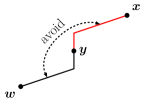
(d) $\bm{y}$ is pivotal.

Figure 2: Schematic representations of the correlation functions. Each dashed arrow labeled “avoid” means that the concerned clusters do not intersect. In Figure 2(d), for example, $\tilde{\mathcal{C}}^{\bm{y}}(\bm{w})$ (in black) and $\tilde{\mathcal{C}}^{\bm{y}}(\bm{x})$ (in red) do not intersect.

By the notion of connectivity (by $(\bm{\psi}_{1},\bm{\psi}_{2},\bm{m})$-open paths), the fourth Ursell function $F_{4}(\bm{w},\bm{x},\bm{y},\bm{z})$ in (4.1) may be illustrated as a connected component containing all four points, as in Figure 2(a). Similarly, the truncated four-point function $\langle S^{\scriptscriptstyle(3)}_{w}(t_{\bm{w}})\,S^{\scriptscriptstyle(3)}_{x}(t_{\bm{x}})\,;S^{\scriptscriptstyle(3)}_{y}(t_{\bm{y}})\,S^{\scriptscriptstyle(3)}_{z}(t_{\bm{z}})\rangle_{\Lambda}$, the three-point function $F_{3}(\bm{w},\bm{x},\bm{y})$ and the cross-correlation function $\langle S^{\scriptscriptstyle(3)}_{w}(t_{\bm{w}})\,S^{\scriptscriptstyle(3)}_{x}(t_{\bm{x}})\,;S^{\scriptscriptstyle(1)}_{y}(t_{\bm{y}})\rangle_{\Lambda}$ in (4.1)–(4.1) may be illustrated as in Figures 2(b), 2(c) and 2(d), respectively.

(a) $\bm{w}\in\mathcal{C}(\bm{z})$.

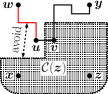
(b) The bridge $(\bm{u},\bm{v})$ is pivotal.

(c) The mark $\bm{v}$ is pivotal.

Figure 3: Decomposition of the event $\{\bm{w}\underset{3,4}{\overset{\mathcal{C}(\bm{z})}{\longleftrightarrow}}\bm{y}\}$, assuming $\mathcal{C}(\bm{z})$ is a fixed set. In Figure 3(b), $\tilde{\mathcal{C}}^{\{\bm{u},\bm{v}\}}(\bm{w})$ (in red) and $\mathcal{C}(\bm{z})$ do not intersect. In Figure 3(c), $\tilde{\mathcal{C}}^{\bm{v}}(\bm{w})$ (in red) and $\mathcal{C}(\bm{z})$ do not intersect.

To explain the inequality (4.1), we first rewrite $F_{4}(\bm{w},\bm{x},\bm{y},\bm{z})$. By the stochastic-geometric representation and repeated use of the source switching, we obtain

$$F_{4}(\bm{w},\bm{x},\bm{y},\bm{z}) =\frac{1}{Z}\mathbb{E}\bigg{[}\sum_{\partial\bm{\psi}=\bm{w}\vartriangle\bm{x}\vartriangle\bm{y}\vartriangle\bm{z}}1\bigg{]}-\frac{1}{Z^{2}}\mathbb{E}^{1}\mathbb{E}^{2}\Bigg{[}\sum_{\begin{subarray}{c}\partial\bm{\psi}_{1}=\bm{w}\vartriangle\bm{x}\\ \partial\bm{\psi}_{2}=\bm{y}\vartriangle\bm{z}\end{subarray}}1\Bigg{]}-G(\bm{w},\bm{y})\,G(\bm{x},\bm{z})-G(\bm{w},\bm{z})\,G(\bm{x},\bm{y})$$

$$=\frac{1}{Z^{2}}\mathbb{E}^{1}\mathbb{E}^{2}\Bigg{[}\sum_{\begin{subarray}{c}\partial\bm{\psi}_{1}=\bm{w}\vartriangle\bm{x}\vartriangle\bm{y}\vartriangle\bm{z}\\ \partial\bm{\psi}_{2}=\varnothing\end{subarray}}\mathbbm{1}{\raisebox{-2.0pt}{$\scriptstyle\{\bm{y}\underset{1,2}{\overset{}{\centernot\longleftrightarrow}}\bm{z}\}$}}\Bigg{]}-G(\bm{w},\bm{y})\,G(\bm{x},\bm{z})-G(\bm{w},\bm{z})\,G(\bm{x},\bm{y})$$

$$=\frac{1}{Z^{2}}\mathbb{E}^{1}\mathbb{E}^{2}\Bigg{[}\sum_{\begin{subarray}{c}\partial\bm{\psi}_{1}=\bm{x}\vartriangle\bm{z}\\ \partial\bm{\psi}_{2}=\bm{w}\vartriangle\bm{y}\end{subarray}}\mathbbm{1}{\raisebox{-2.0pt}{$\scriptstyle\{\bm{y}\underset{1,2}{\overset{}{\centernot\longleftrightarrow}}\bm{z}\}$}}\Bigg{]}-G(\bm{w},\bm{y})\,G(\bm{x},\bm{z})$$

$$\quad+\frac{1}{Z^{2}}\mathbb{E}^{1}\mathbb{E}^{2}\Bigg{[}\sum_{\begin{subarray}{c}\partial\bm{\psi}_{1}=\bm{w}\vartriangle\bm{z}\\ \partial\bm{\psi}_{2}=\bm{x}\vartriangle\bm{y}\end{subarray}}\mathbbm{1}{\raisebox{-2.0pt}{$\scriptstyle\{\bm{y}\underset{1,2}{\overset{}{\centernot\longleftrightarrow}}\bm{z}\}$}}\Bigg{]}-G(\bm{w},\bm{z})\,G(\bm{x},\bm{y}).$$ (4.15)

By the so-called conditioning-on-clusters argument that is heavily used in Section 5, we can rewrite the expectations as

$$\frac{1}{Z^{2}}\mathbb{E}^{1}\mathbb{E}^{2}\Bigg{[}\sum_{\begin{subarray}{c}\partial\bm{\psi}_{1}=\bm{x}\vartriangle\bm{z}\\ \partial\bm{\psi}_{2}=\bm{w}\vartriangle\bm{y}\end{subarray}}\mathbbm{1}{\raisebox{-2.0pt}{$\scriptstyle\{\bm{y}\underset{1,2}{\overset{}{\centernot\longleftrightarrow}}\bm{z}\}$}}\Bigg{]} =\frac{1}{Z^{2}}\mathbb{E}^{1}\mathbb{E}^{2}\Bigg{[}\sum_{\begin{subarray}{c}\partial\bm{\psi}_{1}=\bm{x}\vartriangle\bm{z}\\ \partial\bm{\psi}_{2}=\varnothing\end{subarray}}G_{\mathcal{C}_{1,2}^{\mathrm{c}}}(\bm{w},\bm{y})\Bigg{]},$$ (4.16)

$$\frac{1}{Z^{2}}\mathbb{E}^{1}\mathbb{E}^{2}\Bigg{[}\sum_{\begin{subarray}{c}\partial\bm{\psi}_{1}=\bm{w}\vartriangle\bm{z}\\ \partial\bm{\psi}_{2}=\bm{x}\vartriangle\bm{y}\end{subarray}}\mathbbm{1}{\raisebox{-2.0pt}{$\scriptstyle\{\bm{y}\underset{1,2}{\overset{}{\centernot\longleftrightarrow}}\bm{z}\}$}}\Bigg{]} =\frac{1}{Z^{2}}\mathbb{E}^{1}\mathbb{E}^{2}\Bigg{[}\sum_{\begin{subarray}{c}\partial\bm{\psi}_{1}=\bm{w}\vartriangle\bm{z}\\ \partial\bm{\psi}_{2}=\varnothing\end{subarray}}G_{\mathcal{C}_{1,2}^{\mathrm{c}}}(\bm{x},\bm{y})\Bigg{]},$$ (4.17)

where $\mathcal{C}_{1,2}\equiv\mathcal{C}(\bm{z})$ is random against the outer expectation, but deterministic against the inner expectation. Since (cf., (3.2) and (3.27))

$$G(\bm{w},\bm{y})-G_{\mathcal{C}_{1,2}^{\mathrm{c}}}(\bm{w},\bm{y})=\frac{1}{ZZ_{\mathcal{C}_{1,2}^{\mathrm{c}}}}\mathbb{E}^{3}\mathbb{E}^{4}_{\mathcal{C}_{1,2}^{\mathrm{c}}}\Bigg{[}\sum_{\begin{subarray}{c}\partial\bm{\psi}^{3}=\bm{w}\vartriangle\bm{y}\\ \partial\bm{\psi}^{4}=\varnothing\end{subarray}}\mathbbm{1}{\raisebox{-2.0pt}{$\scriptstyle\{\bm{w}\underset{3,4}{\overset{\mathcal{C}_{1,2}}{\longleftrightarrow}}\bm{y}\}$}}\Bigg{]},$$ (4.18)

we obtain the rewrite

$$F_{4}(\bm{w},\bm{x},\bm{y},\bm{z})={} -\frac{1}{Z^{2}}\mathbb{E}^{1}\mathbb{E}^{2}\bigggl[\sum_{\begin{subarray}{c}\partial\bm{\psi}^{1}=\bm{x}\vartriangle\bm{z}\\ \partial\bm{\psi}^{2}=\varnothing\end{subarray}}\frac{1}{ZZ_{\mathcal{C}_{1,2}^{\mathrm{c}}}}\mathbb{E}^{3}\mathbb{E}^{4}_{\mathcal{C}_{1,2}^{\mathrm{c}}}\Biggl{[}\sum_{\begin{subarray}{c}\partial\bm{\psi}^{3}=\bm{w}\vartriangle\bm{y}\\ \partial\bm{\psi}^{4}=\varnothing\end{subarray}}\mathbbm{1}{\raisebox{-2.0pt}{$\scriptstyle\{\bm{w}\underset{3,4}{\overset{\mathcal{C}_{1,2}}{\longleftrightarrow}}\bm{y}\}$}}\Biggr{]}\bigggr]$$

$$-\frac{1}{Z^{2}}\mathbb{E}^{1}\mathbb{E}^{2}\bigggl[\sum_{\begin{subarray}{c}\partial\bm{\psi}^{1}=\bm{w}\vartriangle\bm{z}\\ \partial\bm{\psi}^{2}=\varnothing\end{subarray}}\frac{1}{ZZ_{\mathcal{C}_{1,2}^{\mathrm{c}}}}\mathbb{E}^{3}\mathbb{E}^{4}_{\mathcal{C}_{1,2}^{\mathrm{c}}}\Biggl{[}\sum_{\begin{subarray}{c}\partial\bm{\psi}^{3}=\bm{x}\vartriangle\bm{y}\\ \partial\bm{\psi}^{4}=\varnothing\end{subarray}}\mathbbm{1}{\raisebox{-2.0pt}{$\scriptstyle\{\bm{x}\underset{3,4}{\overset{\mathcal{C}_{1,2}}{\longleftrightarrow}}\bm{y}\}$}}\Biggr{]}\bigggr]$$ (4.19)

Take the first term on the right, for example, where all $(\bm{\psi}^{3},\bm{\psi}^{4},\bm{m}^{\prime})$-open paths from $\bm{w}$ to $\bm{y}$ must go through $\mathcal{C}_{1,2}$. This is realized in three disjoint cases: (a) $\bm{w}\in\mathcal{C}_{1,2}$ (cf., Figure 3(a)), (b) $\exists(\bm{u},\bm{v})\in\texttt{piv}\{\bm{w}\underset{3,4}{\overset{}{\longleftrightarrow}}\bm{y}\}$ such that $\tilde{\mathcal{C}}_{3,4}^{\{\bm{u},\bm{v}\}}(\bm{w})\cap\mathcal{C}_{1,2}=\varnothing$ (cf., Figure 3(b)) and (c) $\exists$a pivotal mark $\bm{v}$ such that $\tilde{\mathcal{C}}_{3,4}^{\scriptscriptstyle\bm{v}}(\bm{w})\cap\mathcal{C}_{1,2}=\varnothing$ (cf., Figure 3(c)). The case (a) corresponds to the first term on the right-hand side of (4.1), while the case (b) and the case (c) correspond to (parts of) the third and fourth terms on the right-hand side of (4.1), respectively.

We can follow the same strategy to obtain the inequality (4.1). Similarly to the above rewrite for $F_{4}(\bm{w},\bm{x},\bm{y},\bm{z})$, we can also obtain the rewrite

$$F_{3}(\bm{w},\bm{x},\bm{y})={} \frac{1}{Z^{2}}\mathbb{E}^{1}\mathbb{E}^{2}\bigggl[\sum_{\begin{subarray}{c}\partial\bm{\psi}^{1}=\bm{y}\vartriangle\bm{x}\\ \partial\bm{\psi}^{2}=\varnothing\end{subarray}}\frac{1}{ZZ_{\mathcal{C}_{1,2}^{\mathrm{c}}}}\mathbb{E}^{3}\mathbb{E}^{4}_{\mathcal{C}_{1,2}^{\mathrm{c}}}\Biggl{[}\sum_{\begin{subarray}{c}\partial\bm{\psi}^{3}=\bm{w}\vartriangle\bm{y}\\ \partial\bm{\psi}^{4}=\varnothing\end{subarray}}\mathbbm{1}{\raisebox{-2.0pt}{$\scriptstyle\{\bm{w}\underset{3,4}{\overset{\mathcal{C}_{1,2}}{\longleftrightarrow}}\bm{y}\}$}}\Biggr{]}\bigggr]$$

$$+\frac{1}{Z^{2}}\mathbb{E}^{1}\mathbb{E}^{2}\bigggl[\sum_{\begin{subarray}{c}\partial\bm{\psi}^{1}=\bm{y}\vartriangle\bm{w}\\ \partial\bm{\psi}^{2}=\varnothing\end{subarray}}\frac{1}{ZZ_{\mathcal{C}_{1,2}^{\prime\mathrm{c}}}}\mathbb{E}^{3}\mathbb{E}^{4}_{\mathcal{C}_{1,2}^{\prime\mathrm{c}}}\Biggl{[}\sum_{\begin{subarray}{c}\partial\bm{\psi}^{3}=\bm{x}\vartriangle\bm{y}\\ \partial\bm{\psi}^{4}=\varnothing\end{subarray}}\mathbbm{1}{\raisebox{-2.0pt}{$\scriptstyle\{\bm{x}\underset{3,4}{\overset{\mathcal{C}_{1,2}^{\prime}}{\longleftrightarrow}}\bm{y}\}$}}\Biggr{]}\bigggr].$$ (4.20)

where $\mathcal{C}_{1,2}=\tilde{\mathcal{C}}^{\bm{y}}(\bm{x})$ for this case and $\mathcal{C}_{1,2}^{\prime}=\tilde{\mathcal{C}}^{\bm{y}}(\bm{w})$. Then we decompose the event $\{\bm{w}\underset{3,4}{\overset{\mathcal{C}_{1,2}}{\longleftrightarrow}}\bm{y}\}$ into three disjoint cases, as depicted in Figure 4.

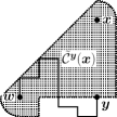
(a) $\bm{w}\in\tilde{\mathcal{C}}^{\bm{y}}(\bm{x})$.

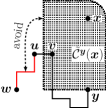
(b) The bridge $(\bm{u},\bm{v})$ is pivotal.

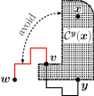
(c) The mark $\bm{v}$ is pivotal.

Figure 4: Decomposition of the event $\{\bm{w}\underset{3,4}{\overset{\tilde{\mathcal{C}}^{\bm{y}}(\bm{x})}{\longleftrightarrow}}\bm{y}\}$, assuming $\tilde{\mathcal{C}}^{\bm{y}}(\bm{x})$ is a fixed set. In Figure 4(b), $\tilde{\mathcal{C}}^{\{\bm{u},\bm{v}\}}(\bm{w})$ (in red) and $\tilde{\mathcal{C}}^{\bm{y}}(\bm{x})$ do not intersect. In Figure 4(c), $\tilde{\mathcal{C}}^{\bm{v}}(\bm{w})$ (in red) and $\tilde{\mathcal{C}}^{\bm{y}}(\bm{x})$ do not intersect.

5 New lace expansion for the classical Ising model

As another example of application of the stochastic-geometric representation and the source switching explained in Section 3, we will derive the lace expansion for $q=0$ (cf., Theorem 5.1 below), which is a new lace expansion for the classical Ising model. The lace expansion for $q>0$ is far more involved, due to pivotal intervals (cf., pivotal bridges in Definition 4.2(iii) below), and will be reported separately in the sequel [21].

The lace expansion is one of the few methods to rigorously prove critical behavior in high dimensions for various models, such as self-avoiding walk [10, 18], lattice trees and lattice animals [17], percolation [16], the classical Ising model [31, 33] and the lattice $\varphi^{4}$ model [32, 9]. David Brydges, who established the methodology of the lace expansion for the first time in 1985 with Thomas Spencer, was awarded the Henri Poincaré Prize in 2024. One of the implications of the lace expansion is an infrared bound on the two-point function, which is uniform in the subcritical regime, without assuming reflection positivity. In the sequel [21], we will show an infrared bound for the quantum Ising model without assuming reflection positivity, which was assumed in the previous section to prove mean-field divergence of the susceptibility.

Let us roughly explain how to derive an infrared bound for the classical Ising model. From now on, we fix $q=0$. In Section 5.1, we will show that the finite-volume two-point function $G(\bm{o},\bm{x})$ obeys the recursion equation

$$G(\bm{o},\bm{x})=\pi^{\scriptscriptstyle(\leq j)}(\bm{o},\bm{x})+\int_{\mathbb{T}}\mathrm{d}t\sum_{\begin{subarray}{c}(\bm{y},\bm{z}):\\ t_{\bm{y}}=t_{\bm{z}}=t\end{subarray}}\beta J_{y,z}\,\pi^{\scriptscriptstyle(\leq j)}(\bm{o},\bm{y})\,G(\bm{z},\bm{x})+(-1)^{j+1}R^{\scriptscriptstyle(j+1)}(\bm{o},\bm{x}),$$ (5.1)

where $\pi^{\scriptscriptstyle(\leq j)}(\bm{o},\bm{x})$ is the $j^{\text{th}}$ partial sum of the alternating series of the nonnegative expansion coefficients $\{\pi^{\scriptscriptstyle(i)}(\bm{o},\bm{x})\}_{i=0}^{\infty}$, i.e., $\pi^{\scriptscriptstyle(\leq j)}(\bm{o},\bm{x})=\sum_{i=0}^{j}(-1)^{i}\pi^{\scriptscriptstyle(i)}(\bm{o},\bm{x})$; $R^{\scriptscriptstyle(j+1)}(\bm{o},\bm{x})\geq 0$ is a remainder. Suppose that $\Lambda$ is the $d$-dimensional hypercube with the periodic boundary condition (i.e., the opposite faces of $\Lambda$ are regarded as identical). Let $\hat{G}(\omega,k)$ be the Fourier transform of $G(\bm{o},\bm{x})$: for $\omega\in 2\pi\mathbb{Z}$ and $k\in[-\pi,\pi]^{d}$,

$$\hat{G}(\omega,k)=\int_{\mathbb{T}}\mathrm{d}t\sum_{x\in\Lambda}e^{\mathrm{i}\omega t+\mathrm{i}k\cdot x}G\big{(}\bm{o},(t,x)\big{)}.$$ (5.2)

Similarly define $\hat{\pi}^{\scriptscriptstyle(\leq j)}(\omega,k)$ and $\hat{R}^{\scriptscriptstyle(j)}(\omega,k)$. Suppose further that there is an infinite-volume limit $\hat{\pi}(\omega,k)=\lim_{\Lambda\uparrow\mathbb{Z}^{d}}\lim_{j\uparrow\infty}\hat{\pi}^{\scriptscriptstyle(\leq j)}(\omega,k)$ and $\lim_{\Lambda\uparrow\mathbb{Z}^{d}}\lim_{j\uparrow\infty}\hat{R}^{\scriptscriptstyle(j)}(\omega,k)=0$ for any $(\omega,k)$ and $\beta<\beta_{\mathrm{c}}\equiv\beta_{\mathrm{c}}(0)$, which can be verified eventually for $d\gg 4$, or for sufficiently spread-out models with $d>4$. Then we obtain

$$\hat{G}(\omega,k)=\hat{\pi}(\omega,k)+\beta\hat{J}(k)\,\hat{\pi}(\omega,k)\,\hat{G}(\omega,k)=\frac{\hat{\pi}(\omega,k)}{1-\beta\hat{J}(k)\,\hat{\pi}(\omega,k)},$$ (5.3)

where $\hat{J}(k)=\sum_{x}e^{\mathrm{i}k\cdot x}J_{o,x}$. Suppose that $\hat{\pi}(\omega,k)$ is bounded away from zero and infinity, uniformly in $\beta<\beta_{\mathrm{c}}$, which can also be verified for $d\gg 4$ or for sufficiently spread-out models with $d>4$. Then, since $\chi=\hat{G}(0,0)$, we obtain

$$\hat{G}(\omega,k)=\frac{1}{\hat{\pi}(\omega,k)^{-1}-\beta\hat{J}(k)}=\frac{1}{\chi^{-1}-\hat{\pi}(0,0)^{-1}+\beta\hat{J}(0)+\hat{\pi}(\omega,k)^{-1}-\beta\hat{J}(k)}$$

$$=\Bigg{(}\chi^{-1}-\hat{\pi}(0,0)^{-1}+\hat{\pi}(\omega,0)^{-1}+\bigg{(}\beta-\frac{\hat{\pi}(\omega,0)^{-1}-\hat{\pi}(\omega,k)^{-1}}{\hat{J}(0)-\hat{J}(k)}\bigg{)}\big{(}\hat{J}(0)-\hat{J}(k)\big{)}\Bigg{)}^{-1},$$ (5.4)

which may imply an infrared bound (cf., (2.3))

$$|\hat{G}(\omega,k)|\lesssim\Bigg{(}\frac{-\partial_{\omega}^{2}\hat{\pi}(0,0)^{-1}}{2}\omega^{2}+\bigg{(}\beta-\frac{\Delta\hat{\pi}(0,0)^{-1}}{\Delta\hat{J}(0)}\bigg{)}\big{(}\hat{J}(0)-\hat{J}(k)\big{)}\Bigg{)}^{-1},$$ (5.5)

assuming existence of the derivatives. Notice that the above argument does not require reflection positivity. Letting $\omega=0$, in particular, yields an infrared bound on the classical Ising two-point function.

Next we derive the lace expansion (5.1) for $q=0$.

5.1 Derivation of the expansion

The 1st stage:

By (3.14) and (3.26) with $\mathcal{C}=\varnothing$, we have

$$G(\bm{o},\bm{x})=\frac{1}{Z^{2}}\mathbb{E}^{1}\mathbb{E}^{2}\Bigg{[}\sum_{\begin{subarray}{c}\partial\bm{\psi}^{1}=\bm{o}\vartriangle\bm{x}\\ \partial\bm{\psi}^{2}=\varnothing\end{subarray}}\mathbbm{1}{\raisebox{-2.0pt}{$\scriptstyle\{\bm{o}\underset{1,2}{\overset{}{\longleftrightarrow}}\bm{x}\}$}}\Bigg{]}.$$ (5.6)

The indicator $\mathbbm{1}{\raisebox{-2.0pt}{$\scriptstyle\{\bm{o}\underset{1,2}{\overset{}{\longleftrightarrow}}\bm{x}\}$}}$ can be split into two, depending on whether $\bm{o}$ is doubly connected to $\bm{x}$ or is not:

$$G(\bm{o},\bm{x})=\pi^{\scriptscriptstyle(0)}(\bm{o},\bm{x})+\frac{1}{Z^{2}}\mathbb{E}^{1}\mathbb{E}^{2}\Bigg{[}\sum_{\begin{subarray}{c}\partial\bm{\psi}^{1}=\bm{o}\vartriangle\bm{x}\\ \partial\bm{\psi}^{2}=\varnothing\end{subarray}}\mathbbm{1}{\raisebox{-2.0pt}{$\scriptstyle\{\bm{o}\underset{1,2}{\overset{}{\longleftrightarrow}}\bm{x}\}\setminus\{\bm{o}\underset{1,2}{\overset{}{\Longleftrightarrow}}\bm{x}\}$}}\Bigg{]},$$ (5.7)

where

$$\pi^{\scriptscriptstyle(0)}(\bm{o},\bm{x})=\frac{1}{Z^{2}}\mathbb{E}^{1}\mathbb{E}^{2}\Bigg{[}\sum_{\begin{subarray}{c}\partial\bm{\psi}^{1}=\bm{o}\vartriangle\bm{x}\\ \partial\bm{\psi}^{2}=\varnothing\end{subarray}}\mathbbm{1}{\raisebox{-2.0pt}{$\scriptstyle\{\bm{o}\underset{1,2}{\overset{}{\Longleftrightarrow}}\bm{x}\}$}}\Bigg{]}.$$ (5.8)

On the event $\{\bm{o}\underset{1,2}{\overset{}{\longleftrightarrow}}\bm{x}\}\setminus\{\bm{o}\underset{1,2}{\overset{}{\Longleftrightarrow}}\bm{x}\}$, there is at least one pivotal bridge for $\bm{o}\underset{1,2}{\overset{}{\longleftrightarrow}}\bm{x}$. Taking the first among those pivotal bridges yields the decomposition

$$\mathbbm{1}{\raisebox{-2.0pt}{$\scriptstyle\{\bm{o}\underset{1,2}{\overset{}{\longleftrightarrow}}\bm{x}\}\setminus\{\bm{o}\underset{1,2}{\overset{}{\Longleftrightarrow}}\bm{x}\}$}}=\sum_{(\bm{u},\bm{v}):\{\bm{u},\bm{v}\}\in\bm{\xi}}\mathbbm{1}{\raisebox{-2.0pt}{$\scriptstyle\{\bm{o}\underset{1,2}{\overset{}{\Longleftrightarrow}}\bm{u}\text{ off }\{\bm{u},\bm{v}\}\}$}}\,\mathbbm{1}{\raisebox{-2.0pt}{$\scriptstyle\{\bm{v}\underset{1,2}{\overset{}{\longleftrightarrow}}\bm{x}\text{ in }\mathcal{C}_{1,2}^{\mathrm{c}}\}$}},$$ (5.9)

where $\bm{\xi}=\bm{\xi}^{1}\cup\bm{\xi}^{2}$ and $\mathcal{C}_{1,2}=\tilde{\mathcal{C}}^{\{\bm{u},\bm{v}\}}(\bm{o})$. Since $\partial\bm{\psi}^{1}=\bm{o}\vartriangle\bm{x}$ and $\partial\bm{\psi}^{2}=\varnothing$, we can replace the sum over $\{\bm{u},\bm{v}\}\in\bm{\xi}$ with that over $\{\bm{u},\bm{v}\}\in\bm{\xi}^{1}$. By the Mecke equation for Poisson point processes, we obtain the rewrite

$$\mathbb{E}^{1}\mathbb{E}^{2}\Bigg{[}\sum_{\begin{subarray}{c}\partial\bm{\psi}^{1}=\bm{o}\vartriangle\bm{x}\\ \partial\bm{\psi}^{2}=\varnothing\end{subarray}}\sum_{\begin{subarray}{c}(\bm{u},\bm{v}):\\ \{\bm{u},\bm{v}\}\in\bm{\xi}^{1}\end{subarray}}\mathbbm{1}{\raisebox{-2.0pt}{$\scriptstyle\{\bm{o}\underset{1,2}{\overset{}{\Longleftrightarrow}}\bm{u}\text{ off }\{\bm{u},\bm{v}\}\}$}}\,\mathbbm{1}{\raisebox{-2.0pt}{$\scriptstyle\{\bm{v}\underset{1,2}{\overset{}{\longleftrightarrow}}\bm{x}\text{ in }\mathcal{C}_{1,2}^{\mathrm{c}}\}$}}\Bigg{]}$$

$$=\int_{\mathbb{T}}\mathrm{d}t\sum_{\begin{subarray}{c}(\bm{u},\bm{v}):\\ t_{\bm{u}}=t_{\bm{v}}=t\end{subarray}}\beta J_{u,v}\,\mathbb{E}^{1}\mathbb{E}^{2}\Bigg{[}\sum_{\begin{subarray}{c}\partial\bm{\psi}^{1}=\bm{o}\vartriangle\bm{x}\vartriangle\{\bm{u},\bm{v}\}\\ \partial\bm{\psi}^{2}=\varnothing\end{subarray}}\mathbbm{1}{\raisebox{-2.0pt}{$\scriptstyle\{\bm{o}\underset{1,2}{\overset{}{\Longleftrightarrow}}\bm{u}\text{ off }\{\bm{u},\bm{v}\}\}$}}\,\mathbbm{1}{\raisebox{-2.0pt}{$\scriptstyle\{\bm{v}\underset{1,2}{\overset{}{\longleftrightarrow}}\bm{x}\text{ in }\mathcal{C}_{1,2}^{\mathrm{c}}\}$}}\Bigg{]}.$$ (5.11)

Conditioning on the cluster $\mathcal{C}_{1,2}$ and splitting each $\bm{\psi}^{j}$ into $\bm{\psi}^{j^{\prime}}\equiv\bm{\psi}^{j}|_{\mathcal{C}_{1,2}}$ and $\bm{\psi}^{j^{\prime\prime}}\equiv\bm{\psi}^{j}|_{\mathcal{C}_{1,2}^{\mathrm{c}}}$, we can further rewrite the expectation on the right-hand side as

$$\mathbb{E}^{1}\mathbb{E}^{2}\Bigg{[}\sum_{\begin{subarray}{c}\partial\bm{\psi}^{1^{\prime}}=\bm{o}\vartriangle\bm{u}\\ \partial\bm{\psi}^{2^{\prime}}=\varnothing\end{subarray}}\mathbbm{1}{\raisebox{-2.0pt}{$\scriptstyle\{\bm{o}\underset{1^{\prime},2^{\prime}}{\overset{}{\Longleftrightarrow}}\bm{u}\text{ off }\{\bm{u},\bm{v}\}\}$}}\sum_{\begin{subarray}{c}\partial\bm{\psi}^{1^{\prime\prime}}=\bm{v}\vartriangle\bm{x}\\ \partial\bm{\psi}^{2^{\prime\prime}}=\varnothing\end{subarray}}\mathbbm{1}{\raisebox{-2.0pt}{$\scriptstyle\{\bm{v}\underset{1^{\prime\prime},2^{\prime\prime}}{\overset{}{\longleftrightarrow}}\bm{x}\text{ in }\mathcal{C}_{1,2}^{\mathrm{c}}\}$}}\Bigg{]}$$

$$=\mathbb{E}^{1^{\prime}}\mathbb{E}^{2^{\prime}}\Bigg{[}\sum_{\begin{subarray}{c}\partial\bm{\psi}^{1^{\prime}}=\bm{o}\vartriangle\bm{u}\\ \partial\bm{\psi}^{2^{\prime}}=\varnothing\end{subarray}}\mathbbm{1}{\raisebox{-2.0pt}{$\scriptstyle\{\bm{o}\underset{1^{\prime},2^{\prime}}{\overset{}{\Longleftrightarrow}}\bm{u}\text{ off }\{\bm{u},\bm{v}\}\}$}}~\mathbb{E}_{\mathcal{C}_{1^{\prime},2^{\prime}}^{\mathrm{c}}}^{1^{\prime\prime}}\mathbb{E}_{\mathcal{C}_{1^{\prime},2^{\prime}}^{\mathrm{c}}}^{2^{\prime\prime}}\Bigg{[}\sum_{\begin{subarray}{c}\partial\bm{\psi}^{1^{\prime\prime}}=\bm{v}\vartriangle\bm{x}\\ \partial\bm{\psi}^{2^{\prime\prime}}=\varnothing\end{subarray}}\mathbbm{1}{\raisebox{-2.0pt}{$\scriptstyle\{\bm{v}\underset{1^{\prime\prime},2^{\prime\prime}}{\overset{}{\longleftrightarrow}}\bm{x}\}$}}\Bigg{]}\Bigg{]},$$ (5.12)

where $\mathcal{C}_{1^{\prime},2^{\prime}}$ is random against the outer expectation $\mathbb{E}^{1^{\prime}}\mathbb{E}^{2^{\prime}}$. Notice that $\mathbbm{1}{\raisebox{-2.0pt}{$\scriptstyle\{\bm{v}\underset{1^{\prime\prime},2^{\prime\prime}}{\overset{}{\longleftrightarrow}}\bm{x}\}$}}=1$ under the source constraint $\partial\bm{\psi}^{1^{\prime\prime}}=\bm{v}\vartriangle\bm{x}$. Therefore,

$$\mathbb{E}_{\mathcal{C}_{1^{\prime},2^{\prime}}^{\mathrm{c}}}^{1^{\prime\prime}}\mathbb{E}_{\mathcal{C}_{1^{\prime},2^{\prime}}^{\mathrm{c}}}^{2^{\prime\prime}}\Bigg{[}\sum_{\begin{subarray}{c}\partial\bm{\psi}^{1^{\prime\prime}}=\bm{v}\vartriangle\bm{x}\\ \partial\bm{\psi}^{2^{\prime\prime}}=\varnothing\end{subarray}}\mathbbm{1}{\raisebox{-2.0pt}{$\scriptstyle\{\bm{v}\underset{1^{\prime\prime},2^{\prime\prime}}{\overset{}{\longleftrightarrow}}\bm{x}\}$}}\Bigg{]}=Z_{\mathcal{C}_{1^{\prime},2^{\prime}}^{\mathrm{c}}}\,\mathbb{E}_{\mathcal{C}_{1^{\prime},2^{\prime}}^{\mathrm{c}}}^{1^{\prime\prime}}\Bigg{[}\sum_{\partial\bm{\psi}^{1^{\prime\prime}}=\bm{v}\vartriangle\bm{x}}1\Bigg{]}=Z_{\mathcal{C}_{1^{\prime},2^{\prime}}^{\mathrm{c}}}^{2}\,G_{\mathcal{C}_{1^{\prime},2^{\prime}}^{\mathrm{c}}}(\bm{v},\bm{x})$$

$$=\mathbb{E}_{\mathcal{C}_{1^{\prime},2^{\prime}}^{\mathrm{c}}}^{1^{\prime\prime}}\mathbb{E}_{\mathcal{C}_{1^{\prime},2^{\prime}}^{\mathrm{c}}}^{2^{\prime\prime}}\Bigg{[}\sum_{\partial\bm{\psi}^{1^{\prime\prime}}=\partial\bm{\psi}^{2^{\prime\prime}}=\varnothing}1\Bigg{]}\,G_{\mathcal{C}_{1^{\prime},2^{\prime}}^{\mathrm{c}}}(\bm{v},\bm{x}).$$ (5.13)

Substituting this back into (5.1), we arrive at

$$\frac{1}{Z^{2}}\mathbb{E}^{1}\mathbb{E}^{2}\Bigg{[}\sum_{\begin{subarray}{c}\partial\bm{\psi}^{1}=\bm{o}\vartriangle\bm{x}\vartriangle\{\bm{u},\bm{v}\}\\ \partial\bm{\psi}^{2}=\varnothing\end{subarray}}\mathbbm{1}{\raisebox{-2.0pt}{$\scriptstyle\{\bm{o}\underset{1,2}{\overset{}{\Longleftrightarrow}}\bm{u}\text{ off }\{\bm{u},\bm{v}\}\}$}}\,\mathbbm{1}{\raisebox{-2.0pt}{$\scriptstyle\{\bm{v}\underset{1,2}{\overset{}{\longleftrightarrow}}\bm{x}\text{ in }\mathcal{C}_{1,2}^{\mathrm{c}}\}$}}\Bigg{]}$$

$$=\frac{1}{Z^{2}}\mathbb{E}^{1}\mathbb{E}^{2}\Bigg{[}\sum_{\begin{subarray}{c}\partial\bm{\psi}^{1}=\bm{o}\vartriangle\bm{u}\\ \partial\bm{\psi}^{2}=\varnothing\end{subarray}}\mathbbm{1}{\raisebox{-2.0pt}{$\scriptstyle\{\bm{o}\underset{1,2}{\overset{}{\Longleftrightarrow}}\bm{u}\}$}}\,G_{\mathcal{C}_{1,2}^{\mathrm{c}}}(\bm{v},\bm{x})\Bigg{]}$$

$$=\pi^{\scriptscriptstyle(0)}(\bm{o},\bm{u})\,G(\bm{v},\bm{x})-\frac{1}{Z^{2}}\mathbb{E}^{1}\mathbb{E}^{2}\Bigg{[}\sum_{\begin{subarray}{c}\partial\bm{\psi}^{1}=\bm{o}\vartriangle\bm{u}\\ \partial\bm{\psi}^{2}=\varnothing\end{subarray}}\mathbbm{1}{\raisebox{-2.0pt}{$\scriptstyle\{\bm{o}\underset{1,2}{\overset{}{\Longleftrightarrow}}\bm{u}\}$}}\,\Big{(}G(\bm{v},\bm{x})-G_{\mathcal{C}_{1,2}^{\mathrm{c}}}(\bm{v},\bm{x})\Big{)}\Bigg{]},$$ (5.14)

where, in the second line, we have dropped “off $\{\bm{u},\bm{v}\}$” since $G_{\mathcal{C}_{1,2}^{\mathrm{c}}}(\bm{v},\bm{x})=0$ on the event $\{\bm{v}\in\mathcal{C}_{1,2}\}\supset\{\bm{o}\underset{1,2}{\overset{}{\Longleftrightarrow}}\bm{u}\}\setminus\{\bm{o}\underset{1,2}{\overset{}{\Longleftrightarrow}}\bm{u}\text{ off }\{\bm{u},\bm{v}\}\}$.

Summarizing the above, we obtain

$$G(\bm{o},\bm{x}) =\pi^{\scriptscriptstyle(0)}(\bm{o},\bm{x})+\int_{\mathbb{T}}\mathrm{d}t\sum_{\begin{subarray}{c}(\bm{u},\bm{v}):\\ t_{\bm{u}}=t_{\bm{v}}=t\end{subarray}}\beta J_{u,v}\,\pi^{\scriptscriptstyle(0)}(\bm{o},\bm{u})\,G(\bm{v},\bm{x})-R^{\scriptscriptstyle(1)}(\bm{o},\bm{x}),$$ (5.15)

where

$$R^{\scriptscriptstyle(1)}(\bm{o},\bm{x})=\int_{\mathbb{T}}\mathrm{d}t\sum_{\begin{subarray}{c}(\bm{u},\bm{v}):\\ t_{\bm{u}}=t_{\bm{v}}=t\end{subarray}}\frac{\beta J_{u,v}}{Z^{2}}~\mathbb{E}^{1}\mathbb{E}^{2}\Bigg{[}\sum_{\begin{subarray}{c}\partial\bm{\psi}^{1}=\bm{o}\vartriangle\bm{u}\\ \partial\bm{\psi}^{2}=\varnothing\end{subarray}}\mathbbm{1}{\raisebox{-2.0pt}{$\scriptstyle\{\bm{o}\underset{1,2}{\overset{}{\Longleftrightarrow}}\bm{u}\}$}}\,\Big{(}G(\bm{v},\bm{x})-G_{\mathcal{C}_{1,2}^{\mathrm{c}}}(\bm{v},\bm{x})\Big{)}\Bigg{]}.$$ (5.16)

This completes the first stage of the expansion.

The 2nd stage:

Next we expand the remainder $R^{\scriptscriptstyle(1)}(\bm{o},\bm{x})$. By (3.2) and (3.27), the expectation in (5.16) can be written as

$$\mathbb{E}^{1}\mathbb{E}^{2}\Bigg{[}\sum_{\begin{subarray}{c}\partial\bm{\psi}^{1}=\bm{o}\vartriangle\bm{u}\\ \partial\bm{\psi}^{2}=\varnothing\end{subarray}}\mathbbm{1}{\raisebox{-2.0pt}{$\scriptstyle\{\bm{o}\underset{1,2}{\overset{}{\Longleftrightarrow}}\bm{u}\}$}}\,\frac{1}{ZZ_{\mathcal{C}_{1,2}^{\mathrm{c}}}}\mathbb{E}^{3}\mathbb{E}_{\mathcal{C}_{1,2}^{\mathrm{c}}}^{4}\Bigg{[}\sum_{\begin{subarray}{c}\partial\bm{\psi}^{3}=\bm{v}\vartriangle\bm{x}\\ \partial\bm{\psi}^{4}=\varnothing\end{subarray}}\mathbbm{1}{\raisebox{-2.0pt}{$\scriptstyle\{\bm{v}\underset{3,4}{\overset{\mathcal{C}_{1,2}}{\longleftrightarrow}}\bm{x}\}$}}\Bigg{]}\Bigg{]}.$$ (5.17)

We split the indicator $\mathbbm{1}{\raisebox{-2.0pt}{$\scriptstyle\{\bm{v}\underset{3,4}{\overset{\mathcal{C}_{1,2}}{\longleftrightarrow}}\bm{x}\}$}}$ into two, depending on whether the event $E_{3,4}(\bm{v},\bm{x};\mathcal{C}_{1,2})$ occurs or does not, where

$$E_{3,4}(\bm{v},\bm{x};\mathcal{C}_{1,2})=\big{\{}\bm{v}\underset{3,4}{\overset{\mathcal{C}_{1,2}}{\longleftrightarrow}}\bm{x}\big{\}}\setminus\Big{\{}\exists(\bm{y},\bm{z})\in\texttt{piv}\big{\{}\bm{v}\underset{3,4}{\overset{}{\longrightarrow}}\bm{x}\big{\}}\text{ s.t. }\bm{v}\underset{3,4}{\overset{\mathcal{C}_{1,2}}{\longleftrightarrow}}\bm{y}\Big{\}}.$$ (5.18)

We define the contribution to $R^{\scriptscriptstyle(1)}(\bm{o},\bm{x})$ from $E_{3,4}(\bm{v},\bm{x};\mathcal{C}_{1,2})$ as $\pi^{\scriptscriptstyle(1)}(\bm{o},\bm{x})$:

$$\pi^{\scriptscriptstyle(1)}(\bm{o},\bm{x})$$

$$=\int_{\mathbb{T}}\mathrm{d}t\sum_{\begin{subarray}{c}(\bm{u},\bm{v}):\\ t_{\bm{u}}=t_{\bm{v}}=t\end{subarray}}\frac{\beta J_{u,v}}{Z^{2}}~\mathbb{E}^{1}\mathbb{E}^{2}\Bigg{[}\sum_{\begin{subarray}{c}\partial\bm{\psi}^{1}=\bm{o}\vartriangle\bm{u}\\ \partial\bm{\psi}^{2}=\varnothing\end{subarray}}\mathbbm{1}{\raisebox{-2.0pt}{$\scriptstyle\{\bm{o}\underset{1,2}{\overset{}{\Longleftrightarrow}}\bm{u}\}$}}\,\frac{1}{ZZ_{\mathcal{C}_{1,2}^{\mathrm{c}}}}\mathbb{E}^{3}\mathbb{E}_{\mathcal{C}_{1,2}^{\mathrm{c}}}^{4}\Bigg{[}\sum_{\begin{subarray}{c}\partial\bm{\psi}^{3}=\bm{v}\vartriangle\bm{x}\\ \partial\bm{\psi}^{4}=\varnothing\end{subarray}}\mathbbm{1}{\raisebox{-2.0pt}{$\scriptstyle E_{3,4}(\bm{v},\bm{x};\mathcal{C}_{1,2})$}}\Bigg{]}\Bigg{]}.$$ (5.19)

On the event $\{\bm{v}\underset{3,4}{\overset{\mathcal{C}_{1,2}}{\longleftrightarrow}}\bm{x}\}\setminus E_{3,4}(\bm{v},\bm{x};\mathcal{C}_{1,2})$, which equals

$$\big{\{}\bm{v}\underset{3,4}{\overset{\mathcal{C}_{1,2}}{\longleftrightarrow}}\bm{x}\big{\}}\cap\Big{\{}\exists(\bm{y},\bm{z})\in\texttt{piv}\big{\{}\bm{v}\underset{3,4}{\overset{}{\longrightarrow}}\bm{x}\big{\}}\text{ s.t. }\bm{v}\underset{3,4}{\overset{\mathcal{C}_{1,2}}{\longleftrightarrow}}\bm{y}\Big{\}},$$ (5.20)

we take the first bridge $(\bm{y},\bm{z})\in\texttt{piv}\{\bm{v}\underset{3,4}{\overset{}{\longrightarrow}}\bm{x}\}$ that satisfies $\bm{v}\underset{3,4}{\overset{\mathcal{C}_{1,2}}{\longleftrightarrow}}\bm{y}$. Then we obtain the decomposition

$$\mathbbm{1}{\raisebox{-2.0pt}{$\scriptstyle\{\bm{v}\underset{3,4}{\overset{\mathcal{C}_{1,2}}{\longleftrightarrow}}\bm{x}\}\setminus E_{3,4}(\bm{v},\bm{x};\mathcal{C}_{1,2})$}}=\sum_{(\bm{y},\bm{z}):\{\bm{y},\bm{z}\}\in\bm{\xi}}\mathbbm{1}{\raisebox{-2.0pt}{$\scriptstyle\{E_{3,4}(\bm{v},\bm{y};\mathcal{C}_{1,2})\text{ off }\{\bm{y},\bm{z}\}\}$}}\,\mathbbm{1}{\raisebox{-2.0pt}{$\scriptstyle\{\bm{z}\underset{3,4}{\overset{}{\longleftrightarrow}}\bm{x}\text{ in }\mathcal{C}_{3,4}^{\mathrm{c}}\}$}},$$ (5.21)

where $\bm{\xi}=\bm{\xi}^{3}\cup\bm{\xi}^{4}$ and $\mathcal{C}_{3,4}=\tilde{\mathcal{C}}^{\{\bm{y},\bm{z}\}}(\bm{v})$. Since $\partial\bm{\psi}^{3}=\bm{v}\vartriangle\bm{x}$ and $\partial\bm{\psi}^{4}=\varnothing$, the sum over $\{\bm{y},\bm{z}\}\in\bm{\xi}$ can be replaced by that over $\{\bm{y},\bm{z}\}\in\bm{\xi}^{3}$. By the Mecke equation again, we obtain

$$\mathbb{E}^{3}\mathbb{E}_{\mathcal{C}_{1,2}^{\mathrm{c}}}^{4}\Bigg{[}\sum_{\begin{subarray}{c}\partial\bm{\psi}^{3}=\bm{v}\vartriangle\bm{x}\\ \partial\bm{\psi}^{4}=\varnothing\end{subarray}}\mathbbm{1}{\raisebox{-2.0pt}{$\scriptstyle\{\bm{v}\underset{3,4}{\overset{\mathcal{C}_{1,2}}{\longleftrightarrow}}\bm{x}\}\setminus E_{3,4}(\bm{v},\bm{x};\mathcal{C}_{1,2})$}}\Bigg{]}$$

$$=\mathbb{E}^{3}\mathbb{E}_{\mathcal{C}_{1,2}^{\mathrm{c}}}^{4}\Bigg{[}\sum_{\begin{subarray}{c}\partial\bm{\psi}^{3}=\bm{v}\vartriangle\bm{x}\\ \partial\bm{\psi}^{4}=\varnothing\end{subarray}}\sum_{(\bm{y},\bm{z}):\{\bm{y},\bm{z}\}\in\bm{\xi}^{3}}\mathbbm{1}{\raisebox{-2.0pt}{$\scriptstyle\{E_{3,4}(\bm{v},\bm{y};\mathcal{C}_{1,2})\text{ off }\{\bm{y},\bm{z}\}\}$}}\,\mathbbm{1}{\raisebox{-2.0pt}{$\scriptstyle\{\bm{z}\underset{3,4}{\overset{}{\longleftrightarrow}}\bm{x}\text{ in }\mathcal{C}_{3,4}^{\mathrm{c}}\}$}}\Bigg{]}$$

$$=\int_{\mathbb{T}}\mathrm{d}s\sum_{\begin{subarray}{c}(\bm{y},\bm{z}):\\ t_{\bm{y}}=t_{\bm{z}}=s\end{subarray}}\beta J_{y,z}\,\mathbb{E}^{3}\mathbb{E}_{\mathcal{C}_{1,2}^{\mathrm{c}}}^{4}\Bigg{[}\sum_{\begin{subarray}{c}\partial\bm{\psi}^{3}=\bm{v}\vartriangle\bm{x}\vartriangle\{\bm{y},\bm{z}\}\\ \partial\bm{\psi}^{4}=\varnothing\end{subarray}}\mathbbm{1}{\raisebox{-2.0pt}{$\scriptstyle\{E_{3,4}(\bm{v},\bm{y};\mathcal{C}_{1,2})\text{ off }\{\bm{y},\bm{z}\}\}$}}\,\mathbbm{1}{\raisebox{-2.0pt}{$\scriptstyle\{\bm{z}\underset{3,4}{\overset{}{\longleftrightarrow}}\bm{x}\text{ in }\mathcal{C}_{3,4}^{\mathrm{c}}\}$}}\Bigg{]}.$$ (5.22)

Then, as done in (5.1), we condition on the cluster $\mathcal{C}_{3,4}$ and split each $\bm{\psi}^{j}$ into $\bm{\psi}^{j^{\prime}}\equiv\bm{\psi}^{j}|_{\mathcal{C}_{3,4}}$ and $\bm{\psi}^{j^{\prime\prime}}\equiv\bm{\psi}^{j}|_{\mathcal{C}_{3,4}^{\mathrm{c}}}$, so that we obtain the rewrite of the expectation on the right-hand side as

$$\mathbb{E}^{3}\mathbb{E}_{\mathcal{C}_{1,2}^{\mathrm{c}}}^{4}\Bigg{[}\sum_{\begin{subarray}{c}\partial\bm{\psi}^{3^{\prime}}=\bm{v}\vartriangle\bm{y}\\ \partial\bm{\psi}^{4^{\prime}}=\varnothing\end{subarray}}\mathbbm{1}{\raisebox{-2.0pt}{$\scriptstyle\{E_{3^{\prime},4^{\prime}}(\bm{v},\bm{y};\mathcal{C}_{1,2})\text{ off }\{\bm{y},\bm{z}\}\}$}}\sum_{\begin{subarray}{c}\partial\bm{\psi}^{3^{\prime\prime}}=\bm{z}\vartriangle\bm{x}\\ \partial\bm{\psi}^{4^{\prime\prime}}=\varnothing\end{subarray}}\mathbbm{1}{\raisebox{-2.0pt}{$\scriptstyle\{\bm{z}\underset{3^{\prime\prime},4^{\prime\prime}}{\overset{}{\longleftrightarrow}}\bm{x}\text{ in }\mathcal{C}_{3,4}^{\mathrm{c}}\}$}}\Bigg{]}$$

$$=\mathbb{E}^{3^{\prime}}\mathbb{E}_{\mathcal{C}_{1,2}^{\mathrm{c}}}^{4^{\prime}}\Bigg{[}\sum_{\begin{subarray}{c}\partial\bm{\psi}^{3^{\prime}}=\bm{v}\vartriangle\bm{y}\\ \partial\bm{\psi}^{4^{\prime}}=\varnothing\end{subarray}}\mathbbm{1}{\raisebox{-2.0pt}{$\scriptstyle\{E_{3^{\prime},4^{\prime}}(\bm{v},\bm{y};\mathcal{C}_{1,2})\text{ off }\{\bm{y},\bm{z}\}\}$}}~\mathbb{E}_{\mathcal{C}_{3^{\prime},4^{\prime}}^{\mathrm{c}}}^{3^{\prime\prime}}\mathbb{E}_{\mathcal{C}_{1,2}^{\mathrm{c}}\cap\mathcal{C}_{3^{\prime},4^{\prime}}^{\mathrm{c}}}^{4^{\prime\prime}}\Bigg{[}\sum_{\begin{subarray}{c}\partial\bm{\psi}^{3^{\prime\prime}}=\bm{z}\vartriangle\bm{x}\\ \partial\bm{\psi}^{4^{\prime\prime}}=\varnothing\end{subarray}}\mathbbm{1}{\raisebox{-2.0pt}{$\scriptstyle\{\bm{z}\underset{3^{\prime\prime},4^{\prime\prime}}{\overset{}{\longleftrightarrow}}\bm{x}\}$}}\Bigg{]}\Bigg{]},$$ (5.23)

where $\mathcal{C}_{3^{\prime},4^{\prime}}$ is random against the outer expectation $\mathbb{E}^{3^{\prime}}\mathbb{E}_{\mathcal{C}_{1,2}^{\mathrm{c}}}^{4^{\prime}}$. Since $\mathbbm{1}{\raisebox{-2.0pt}{$\scriptstyle\{\bm{z}\underset{3^{\prime\prime},4^{\prime\prime}}{\overset{}{\longleftrightarrow}}\bm{x}\}$}}=1$ under the source constraint $\partial\bm{\psi}^{3^{\prime\prime}}=\bm{z}\vartriangle\bm{x}$, we obtain

$$\mathbb{E}_{\mathcal{C}_{3^{\prime},4^{\prime}}^{\mathrm{c}}}^{3^{\prime\prime}}\mathbb{E}_{\mathcal{C}_{1,2}^{\mathrm{c}}\cap\mathcal{C}_{3^{\prime},4^{\prime}}^{\mathrm{c}}}^{4^{\prime\prime}}\Bigg{[}\sum_{\begin{subarray}{c}\partial\bm{\psi}^{3^{\prime\prime}}=\bm{z}\vartriangle\bm{x}\\ \partial\bm{\psi}^{4^{\prime\prime}}=\varnothing\end{subarray}}\mathbbm{1}{\raisebox{-2.0pt}{$\scriptstyle\{\bm{z}\underset{3^{\prime\prime},4^{\prime\prime}}{\overset{}{\longleftrightarrow}}\bm{x}\}$}}\Bigg{]}\Bigg{]}=Z_{\mathcal{C}_{3^{\prime},4^{\prime}}^{\mathrm{c}}}Z_{\mathcal{C}_{1,2}^{\mathrm{c}}\cap\mathcal{C}_{3^{\prime},4^{\prime}}^{\mathrm{c}}}G_{\mathcal{C}_{3^{\prime},4^{\prime}}^{\mathrm{c}}}(\bm{z},\bm{x})$$

$$=\mathbb{E}_{\mathcal{C}_{3^{\prime},4^{\prime}}^{\mathrm{c}}}^{3^{\prime\prime}}\mathbb{E}_{\mathcal{C}_{1,2}^{\mathrm{c}}\cap\mathcal{C}_{3^{\prime},4^{\prime}}^{\mathrm{c}}}^{4^{\prime\prime}}\Bigg{[}\sum_{\partial\bm{\psi}^{3^{\prime\prime}}=\partial\bm{\psi}^{4^{\prime\prime}}=\varnothing}1\Bigg{]}\Bigg{]}\,G_{\mathcal{C}_{3^{\prime},4^{\prime}}^{\mathrm{c}}}(\bm{z},\bm{x}),$$ (5.24)

so that

$$(\ref{eq:nested2}) =\mathbb{E}^{3}\mathbb{E}_{\mathcal{C}_{1,2}^{\mathrm{c}}}^{4}\Bigg{[}\sum_{\begin{subarray}{c}\partial\bm{\psi}^{3}=\bm{v}\vartriangle\bm{y}\\ \partial\bm{\psi}^{4}=\varnothing\end{subarray}}\mathbbm{1}{\raisebox{-2.0pt}{$\scriptstyle E_{3,4}(\bm{v},\bm{y};\mathcal{C}_{1,2})$}}\,G_{\mathcal{C}_{3,4}^{\mathrm{c}}}(\bm{z},\bm{x})\Bigg{]}$$

$$=\mathbb{E}^{3}\mathbb{E}_{\mathcal{C}_{1,2}^{\mathrm{c}}}^{4}\Bigg{[}\sum_{\begin{subarray}{c}\partial\bm{\psi}^{3}=\bm{v}\vartriangle\bm{y}\\ \partial\bm{\psi}^{4}=\varnothing\end{subarray}}\mathbbm{1}{\raisebox{-2.0pt}{$\scriptstyle E_{3,4}(\bm{v},\bm{y};\mathcal{C}_{1,2})$}}\Bigg{]}\,G(\bm{z},\bm{x})$$

$$\quad-\mathbb{E}^{3}\mathbb{E}_{\mathcal{C}_{1,2}^{\mathrm{c}}}^{4}\Bigg{[}\sum_{\begin{subarray}{c}\partial\bm{\psi}^{3}=\bm{v}\vartriangle\bm{y}\\ \partial\bm{\psi}^{4}=\varnothing\end{subarray}}\mathbbm{1}{\raisebox{-2.0pt}{$\scriptstyle E_{3,4}(\bm{v},\bm{y};\mathcal{C}_{1,2})$}}\,\Big{(}G(\bm{z},\bm{x})-G_{\mathcal{C}_{3,4}^{\mathrm{c}}}(\bm{z},\bm{x})\Big{)}\Bigg{]},$$ (5.25)

where, in the first line, we have dropped “off $\{\bm{y},\bm{z}\}$” since $G_{\mathcal{C}_{3,4}^{\mathrm{c}}}(\bm{z},\bm{x})=0$ on the event $\{\bm{z}\in\mathcal{C}_{3,4}\}\supset E_{3,4}(\bm{v},\bm{y};\mathcal{C}_{1,2})\setminus\{E_{3,4}(\bm{v},\bm{y};\mathcal{C}_{1,2})\text{ off }\{\bm{y},\bm{z}\}\}$. Substituting this back into (5.1) and using (5.16) and (5.1), we arrive at

$$R^{\scriptscriptstyle(1)}(\bm{o},\bm{x})=\pi^{\scriptscriptstyle(1)}(\bm{o},\bm{x})+\int_{\mathbb{T}}\mathrm{d}s\sum_{\begin{subarray}{c}(\bm{y},\bm{z}):\\ t_{\bm{y}}=t_{\bm{z}}=s\end{subarray}}\beta J_{y,z}\,\pi^{\scriptscriptstyle(1)}(\bm{o},\bm{y})\,G(\bm{z},\bm{x})-R^{\scriptscriptstyle(2)}(\bm{o},\bm{x}),$$ (5.26)

where

$$R^{\scriptscriptstyle(2)}(\bm{o},\bm{x}) =\int_{\mathbb{T}}\mathrm{d}t\sum_{\begin{subarray}{c}(\bm{u},\bm{v}):\\ t_{\bm{u}}=t_{\bm{v}}=t\end{subarray}}\beta J_{u,v}\int_{\mathbb{T}}\mathrm{d}s\sum_{\begin{subarray}{c}(\bm{y},\bm{z}):\\ t_{\bm{y}}=t_{\bm{z}}=s\end{subarray}}\beta J_{y,z}~\frac{1}{Z^{2}}\mathbb{E}^{1}\mathbb{E}^{2}\Bigg{[}\sum_{\begin{subarray}{c}\partial\bm{\psi}^{1}=\bm{o}\vartriangle\bm{u}\\ \partial\bm{\psi}^{2}=\varnothing\end{subarray}}\mathbbm{1}{\raisebox{-2.0pt}{$\scriptstyle\{\bm{o}\underset{1,2}{\overset{}{\Longleftrightarrow}}\bm{u}\}$}}$$

$$\qquad\times\frac{1}{ZZ_{\mathcal{C}_{1,2}^{\mathrm{c}}}}\mathbb{E}^{3}\mathbb{E}_{\mathcal{C}_{1,2}^{\mathrm{c}}}^{4}\Bigg{[}\sum_{\begin{subarray}{c}\partial\bm{\psi}^{3}=\bm{v}\vartriangle\bm{y}\\ \partial\bm{\psi}^{4}=\varnothing\end{subarray}}\mathbbm{1}{\raisebox{-2.0pt}{$\scriptstyle E_{3,4}(\bm{v},\bm{y};\mathcal{C}_{1,2})$}}\,\Big{(}G(\bm{z},\bm{x})-G_{\mathcal{C}_{3,4}^{\mathrm{c}}}(\bm{z},\bm{x})\Big{)}\Bigg{]}\Bigg{]}.$$ (5.27)

Notice that the difference of the two-point function and its restricted version shows up again. By repeated use of (3.2) and (3.27) and following the same argument as above, we obtain the lace expansion for $q=0$ as follows:

Theorem 5.1 (The lace expansion for $q=0$).

For $j\geq 0$, we let

$$\pi^{\scriptscriptstyle(j)}(\bm{o},\bm{x}) =\int_{\mathbb{T}}\mathrm{d}t_{1}\sum_{\begin{subarray}{c}(\bm{y}_{1},\bm{z}_{1}):\\ t_{\bm{y}_{1}}=t_{\bm{z}_{1}}=t_{1}\end{subarray}}\beta J_{y_{1},z_{1}}\cdots\int_{\mathbb{T}}\mathrm{d}t_{j}\sum_{\begin{subarray}{c}(\bm{y}_{j},\bm{z}_{j}):\\ t_{\bm{y}_{j}}=t_{\bm{z}_{j}}=t_{j}\end{subarray}}\beta J_{y_{j},z_{j}}\frac{1}{Z^{2}}\mathbb{E}^{1}\mathbb{E}^{2}\Bigg{[}\sum_{\begin{subarray}{c}\partial\bm{\psi}^{1}=\bm{o}\vartriangle\bm{y}_{1}\\ \partial\bm{\psi}^{2}=\varnothing\end{subarray}}\mathbbm{1}{\raisebox{-2.0pt}{$\scriptstyle\{\bm{o}\underset{1,2}{\overset{}{\Longleftrightarrow}}\bm{y}_{1}\}$}}$$

$$\quad\times\cdots\frac{1}{ZZ_{\mathcal{C}_{2j-1,2j}^{\mathrm{c}}}}\mathbb{E}^{2j+1}\mathbb{E}_{\mathcal{C}_{2j-1,2j}^{\mathrm{c}}}^{2j+2}\Bigg{[}\sum_{\begin{subarray}{c}\partial\bm{\psi}^{2j+1}=\bm{z}_{j}\vartriangle\bm{x}\\ \partial\bm{\psi}^{2j+2}=\varnothing\end{subarray}}\mathbbm{1}{\raisebox{-2.0pt}{$\scriptstyle E_{2j+1,2j+2}(\bm{z}_{j},\bm{x};\mathcal{C}_{2j-1,2j})$}}\Bigg{]}\cdots\Bigg{]},$$ (5.28)

where $\mathcal{C}_{2j-1,2j}=\tilde{\mathcal{C}}^{\{\bm{y}_{j},\bm{z}_{j}\}}(\bm{z}_{j-1})$ (with $\bm{z}_{0}=\bm{o}$), which is random for $\mathbb{E}^{1}\mathbb{E}^{2}$ when $j=1$ and for $\mathbb{E}^{2j-1}\mathbb{E}_{\mathcal{C}_{2j-3,2j-2}^{\mathrm{c}}}^{2j}$ when $j\geq 2$. Let $\pi^{\scriptscriptstyle(\leq j)}(\bm{o},\bm{x})=\sum_{i=0}^{j}(-1)^{i}\pi^{\scriptscriptstyle(i)}(\bm{o},\bm{x})$. Then, for any $j\geq 0$, the two-point function $G(\bm{o},\bm{x})$ satisfies the recursion equation

$$G(\bm{o},\bm{x})=\pi^{\scriptscriptstyle(\leq j)}(\bm{o},\bm{x})+\int_{\mathbb{T}}\mathrm{d}t\sum_{\begin{subarray}{c}(\bm{y},\bm{z}):\\ t_{\bm{y}}=t_{\bm{z}}=t\end{subarray}}\beta J_{y,z}\,\pi^{\scriptscriptstyle(\leq j)}(\bm{o},\bm{y})\,G(\bm{z},\bm{x})+(-1)^{j+1}R^{\scriptscriptstyle(j+1)}(\bm{o},\bm{x}),$$ (5.29)

where the remainder $R^{\scriptscriptstyle(j+1)}(\bm{o},\bm{x})$ is bounded as

$$0\leq R^{\scriptscriptstyle(j+1)}(\bm{o},\bm{x})\leq\int_{\mathbb{T}}\mathrm{d}t\sum_{\begin{subarray}{c}(\bm{y},\bm{z}):\\ t_{\bm{y}}=t_{\bm{z}}=t\end{subarray}}\beta J_{y,z}\pi^{\scriptscriptstyle(j)}(\bm{o},\bm{y})\,G(\bm{z},\bm{x}).$$ (5.30)

5.2 Diagrammatic bounds on the expansion coefficients

The lace expansion in the previous section is quite similar in spirit to that for the classical Ising model [31]. In [33], we prove diagrammatic bounds on the lace-expansion coefficients by using a “double expansion” i.e., a lace expansion for the expansion coefficients. For example, the $0^{\text{th}}$ expansion coefficient in [31], which is the counterpart to $\pi^{\scriptscriptstyle(0)}(\bm{o},\bm{x})$ in this paper, is defined in terms of the event that there are two disjoint paths of bonds with positive currents between two sources. Since the sum of the currents on the bonds incident on each source is odd, there must be a path of bonds with odd currents joining the two sources. Then we use the “earliest” among such paths as a time line for the double expansion [33, Step 2 in Section 4.1]. In the present setting, since Poisson bridges do not share their endvertices almost surely, there is a unique path ($\subset\texttt{l}(\bm{\psi}^{1})\equiv\{(t,z):\psi^{1}_{z}(t)=\texttt{l}\}$) from $\bm{o}$ to $\bm{x}$ in the bridge configuration $\bm{\xi}^{1}$ almost surely. We call it a backbone, denoted $\mathcal{S}_{1}$, and use it as a “time line” for the double expansion.

In this paper, we explain the aforementioned double expansion by showing a diagrammatic bound on $\pi^{\scriptscriptstyle(0)}(\bm{o},\bm{x})$ in particular. A full proof of diagrammatic bounds on $\pi^{\scriptscriptstyle(j)}(\bm{o},\bm{x})$ for all $j$, including the case of $q>0$, will be reported in the sequel [21].

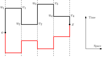
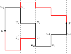
Figure 5: Two examples of $\bm{o}\underset{\mathcal{S}_{1},1^{\prime},2}{\overset{}{\Longleftrightarrow}}\bm{x}$, where $\mathcal{S}_{1}$ is depicted as a path from $\bm{o}$ to $\bm{x}$ (in black). On the left, $\bm{o}$ and $\bm{x}$ are still connected, even after removal of $\mathcal{S}_{1}$, by a $(\bm{\psi}^{1^{\prime}},\bm{\psi}^{2},\bm{0})$-open path (in red), while on the right, they are not. Since $\bm{z}_{1}$ is located in the middle of an interval, there must be a bridge $\{\bm{z}^{\prime}_{1},\bm{z}_{1}\}\in\bm{\xi}^{2}$ such that $\bm{o}\underset{1^{\prime},2}{\overset{}{\longleftrightarrow}}\bm{z}^{\prime}_{1}$ in $\mathcal{S}_{1}^{\mathrm{c}}$.

First, by conditioning on the backbone $\mathcal{S}_{1}$, we can rewrite $\pi^{\scriptscriptstyle(0)}(\bm{o},\bm{x})$ as

$$\pi^{\scriptscriptstyle(0)}(\bm{o},\bm{x}) =\frac{1}{Z^{2}}\mathbb{E}^{1}\Bigg{[}\sum_{\partial\bm{\psi}^{1}=\bm{o}\vartriangle\bm{x}}\mathbb{E}^{2}\bigg{[}\sum_{\partial\bm{\psi}^{2}=\varnothing}\mathbbm{1}{\raisebox{-2.0pt}{$\scriptstyle\{\bm{o}\underset{1,2}{\overset{}{\Longleftrightarrow}}\bm{x}\}$}}\Bigg{]}\Bigg{]}$$

$$=\frac{1}{Z^{2}}\mathbb{E}^{1}\Bigg{[}\sum_{\partial\bm{\psi}^{1}=\bm{o}\vartriangle\bm{x}}\frac{1}{Z_{\mathcal{S}_{1}^{\mathrm{c}}}}\mathbb{E}_{\mathcal{S}_{1}^{\mathrm{c}}}^{1^{\prime}}\mathbb{E}^{2}\Bigg{[}\sum_{\partial\bm{\psi}^{1^{\prime}}=\partial\bm{\psi}^{2}=\varnothing}\mathbbm{1}{\raisebox{-2.0pt}{$\scriptstyle\{\bm{o}\underset{\mathcal{S}_{1},1^{\prime},2}{\overset{}{\Longleftrightarrow}}\bm{x}\}$}}\Bigg{]}\Bigg{]},$$ (5.31)

where $\bm{o}\underset{\mathcal{S}_{1},1^{\prime},2}{\overset{}{\Longleftrightarrow}}\bm{x}$ is an abuse of notation meaning that $\bm{o}$ is doubly connected to $\bm{x}$ in the superposition of $(\bm{\xi}^{1^{\prime}},\bm{\psi}^{1^{\prime}})$, $(\bm{\xi}^{2},\bm{\psi}^{2})$ and $\mathcal{S}_{1}$. We note that $\mathcal{S}_{1}$ is random against the outer expectation $\mathbb{E}^{1}$, but deterministic against the inner expectation $\mathbb{E}_{\mathcal{S}_{1}^{\mathrm{c}}}^{1^{\prime}}\mathbb{E}^{2}$ (cf., Figure 5).

Now we use a double expansion. Denote $\bm{y}\stackrel{{\scriptstyle\scriptscriptstyle\mathcal{S}_{1}}}{{<}}\bm{z}$ if $\bm{y}$ is closer to $\bm{o}$ along $\mathcal{S}_{1}$ than $\bm{z}$; we will use below $\max$ and $\min$ as defined by this relationship. Given $(\bm{\xi}^{1^{\prime}},\bm{\psi}^{1^{\prime}})$ and $(\bm{\xi}^{2},\bm{\psi}^{2})$ satisfying $\partial\bm{\psi}^{1^{\prime}}=\partial\bm{\psi}^{2}=\varnothing$, we define a lace $\mathsf{L}_{1^{\prime},2}=\{\bm{y}_{j}\bm{z}_{j}\}_{j=1}^{N}$ as follows (cf., Figure 6):

• First we define

  $$\bm{y}_{1}=\bm{o}, \bm{z}_{1}=\max\Big{\{}\bm{w}\in\mathcal{S}_{1}:\bm{o}\underset{1^{\prime},2}{\overset{}{\longleftrightarrow}}\bm{w}\text{ in }\mathcal{S}_{1}^{\mathrm{c}}\Big{\}},$$ (5.32)

  where “in $\mathcal{S}_{1}^{\mathrm{c}}$” means that an open path from $\bm{o}$ to $\bm{w}$ does not intersect $\mathcal{S}_{1}$ except for the endvertices $\bm{o}$ and $\bm{w}$. If $\bm{z}_{1}=\bm{x}$, then it is done with $\mathsf{L}_{1^{\prime},2}=\{\bm{o}\bm{x}\}$ and $N=1$.

• If $\bm{z}_{1}\stackrel{{\scriptstyle\scriptscriptstyle\mathcal{S}_{1}}}{{<}}\bm{x}$, then there is almost surely a unique $\bm{y}_{2}\bm{z}_{2}$ defined as

  $$\bm{z}_{2} =\max\Big{\{}\bm{w}\in\mathcal{S}_{1}:\exists\bm{w}^{\prime}\stackrel{{\scriptstyle\scriptscriptstyle\mathcal{S}_{1}}}{{<}}\bm{z}_{1}\stackrel{{\scriptstyle\scriptscriptstyle\mathcal{S}_{1}}}{{<}}\bm{w}\text{ such that }\bm{w}^{\prime}\underset{1^{\prime},2}{\overset{}{\longleftrightarrow}}\bm{w}\text{ in }\mathcal{S}_{1}^{\mathrm{c}}\Big{\}},$$ (5.33)

  $$\bm{y}_{2} =\min\Big{\{}\bm{w}^{\prime}\in\mathcal{S}_{1}:\bm{w}^{\prime}\underset{1^{\prime},2}{\overset{}{\longleftrightarrow}}\bm{z}_{2}\text{ in }\mathcal{S}_{1}^{\mathrm{c}}\Big{\}}.$$ (5.34)

  If $\bm{z}_{2}=\bm{x}$, then it is done with $\mathsf{L}_{1^{\prime},2}=\{\bm{o}\bm{z}_{1},\bm{y}_{2}\bm{x}\}$ and $N=2$.

• Repeat this procedure until it reaches $\bm{z}_{N}=\bm{x}$ with $\mathsf{L}_{1^{\prime},2}=\{\bm{y}_{j}\bm{z}_{j}\}_{j=1}^{N}$.

Notice that, due to the above construction, the lace edges $\{\bm{y}_{j}\bm{z}_{j}\}_{j=1}^{N}$ are mutually avoiding. Then we can rewrite (5.2) as

$$\pi^{\scriptscriptstyle(0)}(\bm{o},\bm{x})=\sum_{N=1}^{\infty}\pi_{N}^{\scriptscriptstyle(0)}(\bm{o},\bm{x}),$$ (5.35)

where

$$\pi_{N}^{\scriptscriptstyle(0)}(\bm{o},\bm{x})=\frac{1}{Z^{2}}\mathbb{E}^{1}\Bigg{[}\sum_{\partial\bm{\psi}^{1}=\bm{o}\vartriangle\bm{x}}\frac{1}{Z_{\mathcal{S}_{1}^{\mathrm{c}}}}\mathbb{E}_{\mathcal{S}_{1}^{\mathrm{c}}}^{1^{\prime}}\mathbb{E}^{2}\Bigg{[}\sum_{\partial\bm{\psi}^{1^{\prime}}=\partial\bm{\psi}^{2}=\varnothing}\sum_{\{\bm{y}_{j}\bm{z}_{j}\}_{j=1}^{N}}\mathbbm{1}{\raisebox{-2.0pt}{$\scriptstyle\{\mathsf{L}_{1^{\prime},2}=\{\bm{y}_{j}\bm{z}_{j}\}_{j=1}^{N}\}$}}\Bigg{]}\Bigg{]}.$$ (5.36)

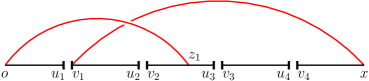
Figure 6: A lace graph corresponding to the right figure in Figure 5. Each line segment (e.g., from $\bm{o}$ to $\bm{u}_{1}$) is an oriented interval in $\mathcal{S}_{1}$, while each gap (e.g., between $\bm{u}_{1}$ and $\bm{v}_{1}$) is a bridge in $\mathcal{S}_{1}$. Since the first lace edge $\bm{o}\bm{z}_{1}$ (in red) lands on the middle of the interval $(\bm{v}_{2},\bm{u}_{3})$, there must be a bridge $\{\bm{z}^{\prime}_{1},\bm{z}_{1}\}\in\bm{\xi}^{2}$ that is not explicitly shown in this figure.

As a first attempt, we investigate the contribution from the case of $N=1$.

Lemma 5.2.

$$\pi_{1}^{\scriptscriptstyle(0)}(\bm{o},\bm{x})\equiv\frac{1}{Z^{2}}\mathbb{E}^{1}\Bigg{[}\sum_{\partial\bm{\psi}^{1}=\bm{o}\vartriangle\bm{x}}\frac{1}{Z_{\mathcal{S}_{1}^{\mathrm{c}}}}\mathbb{E}_{\mathcal{S}_{1}^{\mathrm{c}}}^{1^{\prime}}\mathbb{E}^{2}\Bigg{[}\sum_{\partial\bm{\psi}^{1^{\prime}}=\partial\bm{\psi}^{2}=\varnothing}\mathbbm{1}{\raisebox{-2.0pt}{$\scriptstyle\{\mathsf{L}_{1^{\prime},2}=\{\bm{o}\bm{x}\}\}$}}\Bigg{]}\Bigg{]}\leq G(\bm{o},\bm{x})^{3}.$$ (5.37)

Proof.

By the source switching (cf., Lemma 3.2), we have

$$\frac{1}{Z_{\mathcal{S}_{1}^{\mathrm{c}}}Z}\mathbb{E}_{\mathcal{S}_{1}^{\mathrm{c}}}^{1^{\prime}}\mathbb{E}^{2}\Bigg{[}\sum_{\partial\bm{\psi}^{1^{\prime}}=\partial\bm{\psi}^{2}=\varnothing}\mathbbm{1}{\raisebox{-2.0pt}{$\scriptstyle\{\mathsf{L}_{1^{\prime},2}=\{\bm{o}\bm{x}\}\}$}}\Bigg{]} =\frac{1}{Z_{\mathcal{S}_{1}^{\mathrm{c}}}Z}\mathbb{E}_{\mathcal{S}_{1}^{\mathrm{c}}}^{1^{\prime}}\mathbb{E}^{2}\Bigg{[}\sum_{\partial\bm{\psi}^{1^{\prime}}=\partial\bm{\psi}^{2}=\varnothing}\mathbbm{1}{\raisebox{-2.0pt}{$\scriptstyle\{\bm{o}\underset{1^{\prime},2}{\overset{}{\longleftrightarrow}}\bm{x}\text{ in }\mathcal{S}_{1}^{\mathrm{c}}\}$}}\Bigg{]}$$

$$=\frac{1}{Z_{\mathcal{S}_{1}^{\mathrm{c}}}Z}\mathbb{E}_{\mathcal{S}_{1}^{\mathrm{c}}}^{1^{\prime}}\mathbb{E}^{2}\Bigg{[}\sum_{\partial\bm{\psi}^{1^{\prime}}=\partial\bm{\psi}^{2}=\bm{o}\vartriangle\bm{x}}1\Bigg{]}$$

$$=G_{\mathcal{S}_{1}^{\mathrm{c}}}(\bm{o},\bm{x})\,G(\bm{o},\bm{x}),$$ (5.38)

where the second equality is due to the fact that $\mathbbm{1}{\raisebox{-2.0pt}{$\scriptstyle\{\bm{o}\underset{1^{\prime},2}{\overset{}{\longleftrightarrow}}\bm{x}\text{ in }\mathcal{S}_{1}^{\mathrm{c}}\}$}}=1$ under the constraint $\partial\bm{\psi}^{1^{\prime}}=\partial\bm{\psi}^{2}=\bm{o}\vartriangle\bm{x}$. By monotonicity in terms of the volume, i.e., $G_{\mathcal{S}_{1}^{\mathrm{c}}}(\bm{o},\bm{x})\leq G(\bm{o},\bm{x})$, we obtain

$$\pi_{1}^{\scriptscriptstyle(0)}(\bm{o},\bm{x})\leq\frac{1}{Z}\mathbb{E}^{1}\Bigg{[}\sum_{\partial\bm{\psi}^{1}=\bm{o}\vartriangle\bm{x}}1\Bigg{]}\,G(\bm{o},\bm{x})^{2}=G(\bm{o},\bm{x})^{3},$$ (5.39)

as required. ∎

Next we investigate the contribution from the case of $N=2$. Let

$$(\beta J*G)(\bm{z}_{1},\bm{x})=\sum_{\bm{z}^{\prime}_{1}:t_{\bm{z}^{\prime}_{1}}=t_{\bm{z}_{1}}}\beta J_{z_{1},z^{\prime}_{1}}\,G(\bm{z}^{\prime}_{1},\bm{x}),$$ (5.40)

and define $(G*\beta J)(\bm{z}_{1},\bm{x})$ and $(\beta J*G*\beta J)(\bm{z}_{1},\bm{x})$ similarly.

Lemma 5.3.

$$\pi_{2}^{\scriptscriptstyle(0)}(\bm{o},\bm{x}) \equiv\frac{1}{Z^{2}}\mathbb{E}^{1}\Bigg{[}\sum_{\partial\bm{\psi}^{1}=\bm{o}\vartriangle\bm{x}}\>\sum_{\bm{z}_{1},\bm{y}_{2}}\mathbbm{1}{\raisebox{-2.0pt}{$\scriptstyle\big{\{}\bm{y}_{2}\stackrel{{\scriptstyle\mathcal{S}_{1}}}{{<}}\bm{z}_{1}\big{\}}$}}\,\frac{1}{Z_{\mathcal{S}_{1}^{\mathrm{c}}}}\mathbb{E}_{\mathcal{S}_{1}^{\mathrm{c}}}^{1^{\prime}}\mathbb{E}^{2}\Bigg{[}\sum_{\partial\bm{\psi}^{1^{\prime}}=\partial\bm{\psi}^{2}=\varnothing}\mathbbm{1}{\raisebox{-2.0pt}{$\scriptstyle\{\mathsf{L}_{1^{\prime},2}=\{\bm{o}\bm{z}_{1},\bm{y}_{2}\bm{x}\}\}$}}\Bigg{]}\Bigg{]}$$

$$\leq\iint_{\mathbb{T}\times\mathbb{T}}\mathrm{d}s\,\mathrm{d}t\sum_{\begin{subarray}{c}\bm{z}_{1}:t_{\bm{z}_{1}}=s\\ \bm{y}_{2}:t_{\bm{y}_{2}}=t\end{subarray}}\Big{(}G(\bm{o},\bm{z}_{1})^{2}\,G(\bm{y}_{2},\bm{x})^{2}\,G(\bm{o},\bm{y}_{2})\,(\beta J*G)(\bm{y}_{2},\bm{z}_{1})\,(\beta J*G)(\bm{z}_{1},\bm{x})$$

$$\hskip 108.0pt+[\text{8 other combinations}]\Big{)}.$$ (5.41)

Proof.

Given $\mathcal{S}_{1}$, we say that $\bm{y}$ is type-B if $\bm{y}$ is an endvertex of a bridge in $\mathcal{S}_{1}$ (e.g., $\bm{y}_{2}\equiv\bm{v}_{1}$ in Figure 6), or type-I if $\bm{y}$ is in the middle of an interval in $\mathcal{S}_{1}$ (e.g., $\bm{z}_{1}\in(\bm{v}_{2},\bm{u}_{3})$ in Figure 6). Then, we can rewrite $\pi_{2}^{\scriptscriptstyle(0)}(\bm{o},\bm{x})$ as

$$\frac{1}{Z}\mathbb{E}^{1}\Bigg{[}\sum_{\partial\bm{\psi}^{1}=\bm{o}\vartriangle\bm{x}}\> \sum_{\bm{z}_{1},\bm{y}_{2}}\mathbbm{1}{\raisebox{-2.0pt}{$\scriptstyle\big{\{}\bm{y}_{2}\stackrel{{\scriptstyle\mathcal{S}_{1}}}{{<}}\bm{z}_{1}\big{\}}$}}\Big{(}\mathbbm{1}{\raisebox{-2.0pt}{$\scriptstyle\{\bm{z}_{1}\text{ type-B}\}$}}+\mathbbm{1}{\raisebox{-2.0pt}{$\scriptstyle\{\bm{z}_{1}\text{ type-I}\}$}}\Big{)}\Big{(}\mathbbm{1}{\raisebox{-2.0pt}{$\scriptstyle\{\bm{y}_{2}\text{ type-B}\}$}}+\mathbbm{1}{\raisebox{-2.0pt}{$\scriptstyle\{\bm{y}_{2}\text{ type-I}\}$}}\Big{)}$$

$$\times\frac{1}{Z_{\mathcal{S}_{1}^{\mathrm{c}}}Z}\mathbb{E}_{\mathcal{S}_{1}^{\mathrm{c}}}^{1^{\prime}}\mathbb{E}^{2}\Bigg{[}\sum_{\partial\bm{\psi}^{1^{\prime}}=\partial\bm{\psi}^{2}=\varnothing}\mathbbm{1}{\raisebox{-2.0pt}{$\scriptstyle\{\bm{o}\underset{1^{\prime},2}{\overset{}{\longleftrightarrow}}\bm{z}_{1}\text{ in }\mathcal{S}_{1}^{\mathrm{c}}\}\circ\{\bm{y}_{2}\underset{1^{\prime},2}{\overset{}{\longleftrightarrow}}\bm{x}\text{ in }\mathcal{S}_{1}^{\mathrm{c}}\}$}}\Bigg{]}\Bigg{]},$$ (5.42)

where we have used “$\circ$” to mean that the two events occur “without touching each other” i.e.,

$$\mathbbm{1}{\raisebox{-2.0pt}{$\scriptstyle\{\bm{o}\underset{1^{\prime},2}{\overset{}{\longleftrightarrow}}\bm{z}_{1}\text{ in }\mathcal{S}_{1}^{\mathrm{c}}\}\circ\{\bm{y}_{2}\underset{1^{\prime},2}{\overset{}{\longleftrightarrow}}\bm{x}\text{ in }\mathcal{S}_{1}^{\mathrm{c}}\}$}} =\mathbbm{1}{\raisebox{-2.0pt}{$\scriptstyle\{\bm{o}\underset{1^{\prime},2}{\overset{}{\longleftrightarrow}}\bm{z}_{1}\text{ in }\mathcal{S}_{1}^{\mathrm{c}}\}$}}\,\mathbbm{1}{\raisebox{-2.0pt}{$\scriptstyle\{\bm{y}_{2}\underset{1^{\prime},2}{\overset{}{\longleftrightarrow}}\bm{x}\text{ in }\mathcal{S}_{1}^{\mathrm{c}}\}$}}\,\mathbbm{1}{\raisebox{-2.0pt}{$\scriptstyle\{\tilde{\mathcal{C}}_{1^{\prime},2}^{\mathcal{S}_{1}}(\bm{o})\cap\tilde{\mathcal{C}}_{1^{\prime},2}^{\mathcal{S}_{1}}(\bm{x})=\varnothing\}$}},$$ (5.43)

where $\tilde{\mathcal{C}}_{1^{\prime},2}^{\mathcal{S}_{1}}(\bm{o})=\{\bm{w}\in\mathcal{S}_{1}^{\mathrm{c}}:\bm{o}\underset{1^{\prime},2}{\overset{}{\longleftrightarrow}}\bm{w}$ in $\mathcal{S}_{1}^{\mathrm{c}}\}$. Now we show how to bound the contributions from (i) $\mathbbm{1}{\raisebox{-2.0pt}{$\scriptstyle\{\bm{z}_{1}\text{ type-B}\}$}}\,\mathbbm{1}{\raisebox{-2.0pt}{$\scriptstyle\{\bm{y}_{2}\text{ type-B}\}$}}$ and (ii) $\mathbbm{1}{\raisebox{-2.0pt}{$\scriptstyle\{\bm{z}_{1}\text{ type-I}\}$}}\,\mathbbm{1}{\raisebox{-2.0pt}{$\scriptstyle\{\bm{y}_{2}\text{ type-B}\}$}}$.

(i)  To bound the contribution from $\mathbbm{1}{\raisebox{-2.0pt}{$\scriptstyle\{\bm{z}_{1}\text{ type-B}\}$}}\mathbbm{1}{\raisebox{-2.0pt}{$\scriptstyle\{\bm{y}_{2}\text{ type-B}\}$}}$, we rewrite the inner expectation in (5.2) by conditioning on $\tilde{\mathcal{C}}_{1^{\prime},2}^{\mathcal{S}_{1}}(\bm{o})$ (cf., (5.1)–(5.1) or (5.1)–(5.1)) as

$$\frac{1}{Z_{\mathcal{S}_{1}^{\mathrm{c}}}Z}\mathbb{E}_{\mathcal{S}_{1}^{\mathrm{c}}}^{1^{\prime}}\mathbb{E}^{2}\Bigg{[}\sum_{\partial\bm{\psi}^{1^{\prime}}=\partial\bm{\psi}^{2}=\varnothing}\mathbbm{1}{\raisebox{-2.0pt}{$\scriptstyle\{\bm{o}\underset{1^{\prime},2}{\overset{}{\longleftrightarrow}}\bm{z}_{1}\text{ in }\mathcal{S}_{1}^{\mathrm{c}}\}\circ\{\bm{y}_{2}\underset{1^{\prime},2}{\overset{}{\longleftrightarrow}}\bm{x}\text{ in }\mathcal{S}_{1}^{\mathrm{c}}\}$}}\Bigg{]}$$

$$=\frac{1}{Z_{\mathcal{S}_{1}^{\mathrm{c}}}Z}\mathbb{E}_{\mathcal{S}_{1}^{\mathrm{c}}}^{1^{\prime}}\mathbb{E}^{2}\Bigg{[}\sum_{\partial\bm{\psi}^{1^{\prime}}=\partial\bm{\psi}^{2}=\varnothing}\mathbbm{1}{\raisebox{-2.0pt}{$\scriptstyle\{\bm{o}\underset{1^{\prime},2}{\overset{}{\longleftrightarrow}}\bm{z}_{1}\text{ in }\mathcal{S}_{1}^{\mathrm{c}}\}$}}\,\frac{1}{Z_{\mathcal{S}_{1}^{\mathrm{c}}\cap\tilde{\mathcal{C}}_{1^{\prime},2}^{\mathcal{S}_{1}}(\bm{o})^{\mathrm{c}}}Z_{\tilde{\mathcal{C}}_{1^{\prime},2}^{\mathcal{S}_{1}}(\bm{o})^{\mathrm{c}}}}$$

$$\hskip 84.0pt\times\mathbb{E}^{1^{\prime\prime}}_{\mathcal{S}_{1}^{\mathrm{c}}\cap\tilde{\mathcal{C}}_{1^{\prime},2}^{\mathcal{S}_{1}}(\bm{o})^{\mathrm{c}}}\mathbb{E}^{2^{\prime}}_{\tilde{\mathcal{C}}_{1^{\prime},2}^{\mathcal{S}_{1}}(\bm{o})^{\mathrm{c}}}\Bigg{[}\sum_{\partial\bm{\psi}^{1^{\prime\prime}}=\partial\bm{\psi}^{2^{\prime}}=\varnothing}\mathbbm{1}{\raisebox{-2.0pt}{$\scriptstyle\{\bm{y}_{2}\underset{1^{\prime\prime},2^{\prime}}{\overset{}{\longleftrightarrow}}\bm{x}\text{ in }\mathcal{S}_{1}^{\mathrm{c}}\cap\tilde{\mathcal{C}}_{1^{\prime},2}^{\mathcal{S}_{1}}(\bm{o})^{\mathrm{c}}\}$}}\Bigg{]}\Bigg{]},$$ (5.44)

which is bounded, by using the source switching and monotonicity, by

$$\frac{1}{Z_{\mathcal{S}_{1}^{\mathrm{c}}}Z}\mathbb{E}_{\mathcal{S}_{1}^{\mathrm{c}}}^{1^{\prime}}\mathbb{E}^{2}\Bigg{[}\sum_{\partial\bm{\psi}^{1^{\prime}}=\partial\bm{\psi}^{2}=\varnothing}\mathbbm{1}{\raisebox{-2.0pt}{$\scriptstyle\{\bm{o}\underset{1^{\prime},2}{\overset{}{\longleftrightarrow}}\bm{z}_{1}\text{ in }\mathcal{S}_{1}^{\mathrm{c}}\}$}}\Bigg{]}\,G(\bm{y}_{2},\bm{x})^{2}\leq G(\bm{o},\bm{z}_{1})^{2}\,G(\bm{y}_{2},\bm{x})^{2}.$$ (5.45)

Therefore, the contribution to (5.2) from this case is bounded by

$$\frac{1}{Z}\mathbb{E}^{1}\Bigg{[}\sum_{\partial\bm{\psi}^{1}=\bm{o}\vartriangle\bm{x}}\>\sum_{\bm{z}_{1},\bm{y}_{2}}\mathbbm{1}{\raisebox{-2.0pt}{$\scriptstyle\big{\{}\bm{y}_{2}\stackrel{{\scriptstyle\mathcal{S}_{1}}}{{<}}\bm{z}_{1}\big{\}}$}}\,\mathbbm{1}{\raisebox{-2.0pt}{$\scriptstyle\{\bm{z}_{1}\text{ type-B}\}$}}\,\mathbbm{1}{\raisebox{-2.0pt}{$\scriptstyle\{\bm{y}_{2}\text{ type-B}\}$}}\,G(\bm{o},\bm{z}_{1})^{2}\,G(\bm{y}_{2},\bm{x})^{2}\Bigg{]}.$$ (5.46)

Since $\mathbbm{1}{\raisebox{-2.0pt}{$\scriptstyle\{\bm{z}_{1}\text{ type-B}\}$}}=1$ implies existence of a bridge $\{\bm{z}_{1},\bm{z}^{\prime}_{1}\}\in\bm{\xi}^{1}$ that satisfies $\bm{z}_{1}\stackrel{{\scriptstyle\scriptscriptstyle\mathcal{S}_{1}}}{{<}}\bm{z}^{\prime}_{1}$ or vice versa, we have the rewrite

$$\sum_{\bm{z}_{1},\bm{y}_{2}}\mathbbm{1}{\raisebox{-2.0pt}{$\scriptstyle\{\mathcal{S}_{1}=(\bm{o},\bm{y}_{2})\cdot(\bm{y}_{2},\bm{z}_{1})\cdot(\bm{z}_{1},\bm{x})\}$}}\,\mathbbm{1}{\raisebox{-2.0pt}{$\scriptstyle\{\bm{z}_{1}\text{ type-B}\}$}}\,\mathbbm{1}{\raisebox{-2.0pt}{$\scriptstyle\{\bm{y}_{2}\text{ type-B}\}$}}$$

$$=\sum_{\{\bm{z}_{1},\bm{z}^{\prime}_{1}\},\{\bm{y}_{2},\bm{y}^{\prime}_{2}\}\in\bm{\xi}^{1}}\Big{(}\mathbbm{1}{\raisebox{-2.0pt}{$\scriptstyle\big{\{}\bm{y}_{2}\stackrel{{\scriptstyle\mathcal{S}_{1}}}{{<}}\bm{y}^{\prime}_{2}\stackrel{{\scriptstyle\mathcal{S}_{1}}}{{<}}\bm{z}_{1}\stackrel{{\scriptstyle\mathcal{S}_{1}}}{{<}}\bm{z}^{\prime}_{1}\big{\}}$}}+\mathbbm{1}{\raisebox{-2.0pt}{$\scriptstyle\big{\{}\bm{y}_{2}\stackrel{{\scriptstyle\mathcal{S}_{1}}}{{<}}\bm{y}^{\prime}_{2}\stackrel{{\scriptstyle\mathcal{S}_{1}}}{{<}}\bm{z}^{\prime}_{1}\stackrel{{\scriptstyle\mathcal{S}_{1}}}{{<}}\bm{z}_{1}\big{\}}$}}$$

$$\hskip 120.0pt+\mathbbm{1}{\raisebox{-2.0pt}{$\scriptstyle\big{\{}\bm{y}^{\prime}_{2}\stackrel{{\scriptstyle\mathcal{S}_{1}}}{{<}}\bm{y}_{2}\stackrel{{\scriptstyle\mathcal{S}_{1}}}{{<}}\bm{z}_{1}\stackrel{{\scriptstyle\mathcal{S}_{1}}}{{<}}\bm{z}^{\prime}_{1}\big{\}}$}}+\mathbbm{1}{\raisebox{-2.0pt}{$\scriptstyle\big{\{}\bm{y}^{\prime}_{2}\stackrel{{\scriptstyle\mathcal{S}_{1}}}{{<}}\bm{y}_{2}\stackrel{{\scriptstyle\mathcal{S}_{1}}}{{<}}\bm{z}^{\prime}_{1}\stackrel{{\scriptstyle\mathcal{S}_{1}}}{{<}}\bm{z}_{1}\big{\}}$}}\Big{)}.$$ (5.47)

Then, by the Mecke equation (cf., (5.1)), we can rewrite the contribution from the first indicator as

$$\int_{\mathbb{T}}\mathrm{d}s\sum_{\begin{subarray}{c}\{\bm{z}_{1},\bm{z}^{\prime}_{1}\}:\\ t_{\bm{z}_{1}}=t_{\bm{z}^{\prime}_{1}}=s\end{subarray}}\beta J_{z_{1},z^{\prime}_{1}}\int_{\mathbb{T}}\mathrm{d}t\sum_{\begin{subarray}{c}\{\bm{y}_{2},\bm{y}^{\prime}_{2}\}:\\ t_{\bm{y}_{2}}=t_{\bm{y}^{\prime}_{2}}=t\end{subarray}}\beta J_{y_{2},y^{\prime}_{2}}\,G(\bm{o},\bm{z}_{1})^{2}\,G(\bm{y}_{2},\bm{x})^{2}$$

$$\times\frac{1}{Z}\mathbb{E}^{1}\Bigg{[}\sum_{\partial\bm{\psi}^{1}=\bm{o}\vartriangle\bm{x}\vartriangle\{\bm{z}_{1},\bm{z}^{\prime}_{1}\}\vartriangle\{\bm{y}_{2},\bm{y}^{\prime}_{2}\}}\mathbbm{1}{\raisebox{-2.0pt}{$\scriptstyle\big{\{}\bm{y}_{2}\stackrel{{\scriptstyle\mathcal{S}_{1}}}{{<}}\bm{y}^{\prime}_{2}\stackrel{{\scriptstyle\mathcal{S}_{1}}}{{<}}\bm{z}_{1}\stackrel{{\scriptstyle\mathcal{S}_{1}}}{{<}}\bm{z}^{\prime}_{1}\big{\}}$}}\Bigg{]}.$$ (5.48)

Finally, by conditioning on parts of $\mathcal{S}_{1}$ (cf., (5.2)) and monotonicity, the last line is bounded as

$$\frac{1}{Z}\mathbb{E}^{1}\Bigg{[}\sum_{\partial\bm{\psi}^{1}=\bm{o}\vartriangle\bm{y}_{2}\vartriangle\bm{y}^{\prime}_{2}\vartriangle\bm{z}_{1}}\mathbbm{1}{\raisebox{-2.0pt}{$\scriptstyle\big{\{}\bm{y}_{2}\stackrel{{\scriptstyle\mathcal{S}_{1}}}{{<}}\bm{y}^{\prime}_{2}\stackrel{{\scriptstyle\mathcal{S}_{1}}}{{<}}\bm{z}_{1}\big{\}}$}}\underbrace{\frac{1}{Z_{\mathcal{S}_{1}^{\mathrm{c}}}}\mathbb{E}^{1^{\prime}}_{\mathcal{S}_{1}^{\mathrm{c}}}\Bigg{[}\sum_{\partial\bm{\psi}^{1^{\prime}}=\bm{z}^{\prime}_{1}\vartriangle\bm{x}}\mathbbm{1}{\raisebox{-2.0pt}{$\scriptstyle\{\mathcal{S}_{1}\cap\mathcal{S}_{1^{\prime}}=\varnothing\}$}}\Bigg{]}}_{\leq\,G(\bm{z}^{\prime}_{1},\bm{x})}\Bigg{]}$$

$$\leq\frac{1}{Z}\mathbb{E}^{1}\Bigg{[}\sum_{\partial\bm{\psi}^{1}=\bm{o}\vartriangle\bm{y}_{2}}\underbrace{\frac{1}{Z_{\mathcal{S}_{1}^{\mathrm{c}}}}\mathbb{E}^{1^{\prime}}_{\mathcal{S}_{1}^{\mathrm{c}}}\Bigg{[}\sum_{\partial\bm{\psi}^{1^{\prime}}=\bm{y}^{\prime}_{2}\vartriangle\bm{z}_{1}}\mathbbm{1}{\raisebox{-2.0pt}{$\scriptstyle\{\mathcal{S}_{1}\cap\mathcal{S}_{1^{\prime}}=\varnothing\}$}}\Bigg{]}}_{\leq\,G(\bm{y}^{\prime}_{2},\bm{z}_{1})}\Bigg{]}\,G(\bm{z}^{\prime}_{1},\bm{x})$$

$$\leq G(\bm{o},\bm{y}_{2})\,G(\bm{y}^{\prime}_{2},\bm{z}_{1})\,G(\bm{z}^{\prime}_{1},\bm{x}),$$ (5.49)

where, in the leftmost expression, $\mathcal{S}_{1}$ is the backbone from $\bm{o}$ to $\bm{z}_{1}$, which is random against the outer expectation $\mathbb{E}^{1}$, and $\mathcal{S}_{1^{\prime}}$ is the backbone from $\bm{z}^{\prime}_{1}$ to $\bm{x}$, which is random against the inner expectation $\mathbb{E}^{1^{\prime}}_{\mathcal{S}_{1}^{\mathrm{c}}}$; in the middle expression, $\mathcal{S}_{1}$ is the backbone from $\bm{o}$ to $\bm{y}_{2}$, which is random against the outer expectation $\mathbb{E}^{1}$, and $\mathcal{S}_{1^{\prime}}$ is the backbone from $\bm{y}^{\prime}_{2}$ to $\bm{z}_{1}$, which is random against the inner expectation $\mathbb{E}^{1^{\prime}}_{\mathcal{S}_{1}^{\mathrm{c}}}$. Therefore,

$$(\ref{eq:pi0-N2-cal4})\leq\iint_{\mathbb{T}\times\mathbb{T}}\mathrm{d}s\,\mathrm{d}t\sum_{\begin{subarray}{c}\bm{z}_{1}:t_{\bm{z}_{1}}=s\\ \bm{y}_{2}:t_{\bm{y}_{2}}=t\end{subarray}}G(\bm{o},\bm{z}_{1})^{2}\,G(\bm{y}_{2},\bm{x})^{2}\,G(\bm{o},\bm{y}_{2})\,(\beta J*G)(\bm{y}_{2},\bm{z}_{1})\,(\beta J*G)(\bm{z}_{1},\bm{x}),$$ (5.50)

which already appeared in (5.3).

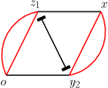
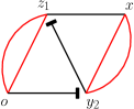
Figure 7: Schematic representation for (5.50) (leftmost) and diagrammatic bounds on the contributions from the other three indicators in (5.2). Each gap represents a bridge, and the four red segments in each figure represent $G(\bm{o},\bm{z}_{1})^{2}\,G(\bm{y}_{2},\bm{x})^{2}$.

The other three cases in (5.2) are bounded similarly by replacing the last three terms in (5.50) by $G(\bm{o},\bm{y}_{2})\,(\beta J*G*\beta J)(\bm{y}_{2},\bm{z}_{1})\,G(\bm{z}_{1},\bm{x})$ (for the $2^{\text{nd}}$ indicator in (5.2)), $(G*\beta J)(\bm{o},\bm{y}_{2})\,G(\bm{y}_{2},\bm{z}_{1})\,(\beta J*G)(\bm{z}_{1},\bm{x})$ (for the $3^{\text{rd}}$ indicator in (5.2)) and $(G*\beta J)(\bm{o},\bm{y}_{2})\,(G*\beta J)(\bm{y}_{2},\bm{z}_{1})\,G(\bm{z}_{1},\bm{x})$ (for the $4^{\text{th}}$ indicator in (5.2)), respectively (cf., Figure 7).

(ii)  To bound the contribution to (5.2) from $\mathbbm{1}{\raisebox{-2.0pt}{$\scriptstyle\{\bm{z}_{1}\text{ type-I}\}$}}\,\mathbbm{1}{\raisebox{-2.0pt}{$\scriptstyle\{\bm{y}_{2}\text{ type-B}\}$}}$, we follow the same strategy as in (i) to bound the inner expectation in (5.2) by the left-hand side of (5.45). Then, we obtain the counterpart to (5.46):

$$\frac{1}{Z}\mathbb{E}^{1}\Bigg{[} \sum_{\partial\bm{\psi}^{1}=\bm{o}\vartriangle\bm{x}}\>\sum_{\bm{z}_{1},\bm{y}_{2}}\mathbbm{1}{\raisebox{-2.0pt}{$\scriptstyle\big{\{}\bm{y}_{2}\stackrel{{\scriptstyle\mathcal{S}_{1}}}{{<}}\bm{z}_{1}\big{\}}$}}\,\mathbbm{1}{\raisebox{-2.0pt}{$\scriptstyle\{\bm{z}_{1}\text{ type-I}\}$}}\,\mathbbm{1}{\raisebox{-2.0pt}{$\scriptstyle\{\bm{y}_{2}\text{ type-B}\}$}}$$

$$\times\frac{1}{Z_{\mathcal{S}_{1}^{\mathrm{c}}}Z}\mathbb{E}_{\mathcal{S}_{1}^{\mathrm{c}}}^{1^{\prime}}\mathbb{E}^{2}\Bigg{[}\sum_{\partial\bm{\psi}^{1^{\prime}}=\partial\bm{\psi}^{2}=\varnothing}\mathbbm{1}{\raisebox{-2.0pt}{$\scriptstyle\{\bm{o}\underset{1^{\prime},2}{\overset{}{\longleftrightarrow}}\bm{z}_{1}\text{ in }\mathcal{S}_{1}^{\mathrm{c}}\}$}}\Bigg{]}\,G(\bm{y}_{2},\bm{x})^{2}\Bigg{]}.$$ (5.51)

Since $\mathbbm{1}{\raisebox{-2.0pt}{$\scriptstyle\{\bm{z}_{1}\text{ type-I}\}$}}=1$ implies existence of a bridge $\{\bm{z}^{\prime}_{1},\bm{z}_{1}\}\in\bm{\xi}^{2}$ that satisfies $\bm{o}\underset{1^{\prime},2}{\overset{}{\longleftrightarrow}}\bm{z}^{\prime}_{1}$ in $\mathcal{S}_{1}^{\mathrm{c}}$ (as explained in Figures 5–6), we can bound (5.2) by

$$\frac{1}{Z}\mathbb{E}^{1}\Bigg{[} \sum_{\partial\bm{\psi}^{1}=\bm{o}\vartriangle\bm{x}}\sum_{\bm{z}_{1}}\sum_{\{\bm{y}_{2},\bm{y}^{\prime}_{2}\}\in\bm{\xi}^{1}}\Big{(}\mathbbm{1}{\raisebox{-2.0pt}{$\scriptstyle\big{\{}\bm{y}_{2}\stackrel{{\scriptstyle\mathcal{S}_{1}}}{{<}}\bm{y}^{\prime}_{2}\stackrel{{\scriptstyle\mathcal{S}_{1}}}{{<}}\bm{z}_{1}\big{\}}$}}+\mathbbm{1}{\raisebox{-2.0pt}{$\scriptstyle\big{\{}\bm{y}^{\prime}_{2}\stackrel{{\scriptstyle\mathcal{S}_{1}}}{{<}}\bm{y}_{2}\stackrel{{\scriptstyle\mathcal{S}_{1}}}{{<}}\bm{z}_{1}\big{\}}$}}\Big{)}$$

$$\times\frac{1}{Z_{\mathcal{S}_{1}^{\mathrm{c}}}Z}\mathbb{E}_{\mathcal{S}_{1}^{\mathrm{c}}}^{1^{\prime}}\mathbb{E}^{2}\Bigg{[}\sum_{\partial\bm{\psi}^{1^{\prime}}=\partial\bm{\psi}^{2}=\varnothing}\sum_{\begin{subarray}{c}\bm{z}^{\prime}_{1}:\\ \{\bm{z}^{\prime}_{1},\bm{z}_{1}\}\in\bm{\xi}^{2}\end{subarray}}\mathbbm{1}{\raisebox{-2.0pt}{$\scriptstyle\{\bm{o}\underset{1^{\prime},2}{\overset{}{\longleftrightarrow}}\bm{z}^{\prime}_{1}\text{ in }\mathcal{S}_{1}^{\mathrm{c}}\}$}}\Bigg{]}\,G(\bm{y}_{2},\bm{x})^{2}\Bigg{]}.$$ (5.52)

Then, by the Mecke equation (cf., (5.1)) and the source switching (cf., Lemma 3.2), we can further bound it by

$$\int_{\mathbb{T}}\mathrm{d}s\sum_{\begin{subarray}{c}\{\bm{z}^{\prime}_{1},\bm{z}_{1}\}:\\ t_{\bm{z}^{\prime}_{1}}=t_{\bm{z}_{1}}=s\end{subarray}}\beta J_{z^{\prime}_{1},z_{1}}\int_{\mathbb{T}}\mathrm{d}t\sum_{\begin{subarray}{c}\{\bm{y}_{2},\bm{y}^{\prime}_{2}\}:\\ t_{\bm{y}_{2}}=t_{\bm{y}^{\prime}_{2}}=t\end{subarray}}\beta J_{y_{2},y^{\prime}_{2}}\,\frac{1}{Z}\mathbb{E}^{1}\Bigg{[}\sum_{\partial\bm{\psi}^{1}=\bm{o}\vartriangle\bm{x}\vartriangle\{\bm{y}_{2},\bm{y}^{\prime}_{2}\}}\Big{(}\mathbbm{1}{\raisebox{-2.0pt}{$\scriptstyle\big{\{}\bm{y}_{2}\stackrel{{\scriptstyle\mathcal{S}_{1}}}{{<}}\bm{y}^{\prime}_{2}\stackrel{{\scriptstyle\mathcal{S}_{1}}}{{<}}\bm{z}_{1}\big{\}}$}}$$

$$\qquad\qquad+\mathbbm{1}{\raisebox{-2.0pt}{$\scriptstyle\big{\{}\bm{y}^{\prime}_{2}\stackrel{{\scriptstyle\mathcal{S}_{1}}}{{<}}\bm{y}_{2}\stackrel{{\scriptstyle\mathcal{S}_{1}}}{{<}}\bm{z}_{1}\big{\}}$}}\Big{)}\underbrace{\frac{1}{Z_{\mathcal{S}_{1}^{\mathrm{c}}}Z}\mathbb{E}_{\mathcal{S}_{1}^{\mathrm{c}}}^{1^{\prime}}\mathbb{E}^{2}\Bigg{[}\sum_{\begin{subarray}{c}\partial\bm{\psi}^{1^{\prime}}=\varnothing\\ \partial\bm{\psi}^{2}=\bm{z}^{\prime}_{1}\vartriangle\bm{z}_{1}\end{subarray}}\mathbbm{1}{\raisebox{-2.0pt}{$\scriptstyle\{\bm{o}\underset{1^{\prime},2}{\overset{}{\longleftrightarrow}}\bm{z}^{\prime}_{1}\text{ in }\mathcal{S}_{1}^{\mathrm{c}}\}$}}\Bigg{]}}_{G_{\mathcal{S}_{1}^{\mathrm{c}}}(\bm{o},\bm{z}^{\prime}_{1})\,G(\bm{o},\bm{z}_{1})~(\because\,\text{Lemma~\ref{lmm:SST}})}G(\bm{y}_{2},\bm{x})^{2}\Bigg{]}$$

$$\leq\iint_{\mathbb{T}\times\mathbb{T}}\mathrm{d}s\,\mathrm{d}t\sum_{\begin{subarray}{c}\bm{z}_{1}:t_{\bm{z}_{1}}=s\\ \bm{y}_{2}:t_{\bm{y}_{2}}=t\end{subarray}}(G*\beta J)(\bm{o},\bm{z}_{1})\,G(\bm{o},\bm{z}_{1})\,G(\bm{y}_{2},\bm{x})^{2}\sum_{\bm{y}^{\prime}_{2}:t_{\bm{y}^{\prime}_{2}}=t}\beta J_{y_{2},y^{\prime}_{2}}$$

$$\qquad\times\frac{1}{Z}\mathbb{E}^{1}\Bigg{[}\sum_{\partial\bm{\psi}^{1}=\bm{o}\vartriangle\bm{x}\vartriangle\{\bm{y}_{2},\bm{y}^{\prime}_{2}\}}\Big{(}\mathbbm{1}{\raisebox{-2.0pt}{$\scriptstyle\big{\{}\bm{y}_{2}\stackrel{{\scriptstyle\mathcal{S}_{1}}}{{<}}\bm{y}^{\prime}_{2}\stackrel{{\scriptstyle\mathcal{S}_{1}}}{{<}}\bm{z}_{1}\big{\}}$}}+\mathbbm{1}{\raisebox{-2.0pt}{$\scriptstyle\big{\{}\bm{y}^{\prime}_{2}\stackrel{{\scriptstyle\mathcal{S}_{1}}}{{<}}\bm{y}_{2}\stackrel{{\scriptstyle\mathcal{S}_{1}}}{{<}}\bm{z}_{1}\big{\}}$}}\Big{)}\Bigg{]}.$$ (5.53)

Finally, by conditioning on parts of the backbone and monotonicity (cf., (5.2)), the last line is bounded by $(G(\bm{o},\bm{y}_{2})\,G(\bm{y}^{\prime}_{2},\bm{z}_{1})+G(\bm{o},\bm{y}^{\prime}_{2})\,G(\bm{y}_{2},\bm{z}_{1}))\,G(\bm{z}_{1},\bm{x})$. As a result, the contribution to (5.2) from $\mathbbm{1}{\raisebox{-2.0pt}{$\scriptstyle\{\bm{z}_{1}\text{ type-I}\}$}}\,\mathbbm{1}{\raisebox{-2.0pt}{$\scriptstyle\{\bm{y}_{2}\text{ type-B}\}$}}$ is bounded by (cf., Figure 8)

$$\iint_{\mathbb{T}\times\mathbb{T}}\mathrm{d}s\,\mathrm{d}t\sum_{\begin{subarray}{c}\bm{z}_{1}:t_{\bm{z}_{1}}=s\\ \bm{y}_{2}:t_{\bm{y}_{2}}=t\end{subarray}}(G*\beta J)(\bm{o},\bm{z}_{1})\,G(\bm{o},\bm{z}_{1})\,G(\bm{y}_{2},\bm{x})^{2}$$

$$\qquad\times\Big{(}G(\bm{o},\bm{y}_{2})\,(\beta J*G)(\bm{y}_{2},\bm{z}_{1})+(G*\beta J)(\bm{o},\bm{y}_{2})\,G(\bm{y}_{2},\bm{z}_{1})\Big{)}\,G(\bm{z}_{1},\bm{x}).$$ (5.54)

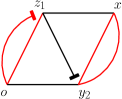
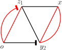
Figure 8: Schematic representation for the two terms in (5.2).

In the same way, we can bound the contribution to (5.2) from $\mathbbm{1}{\raisebox{-2.0pt}{$\scriptstyle\{\bm{z}_{1}\text{ type-B}\}$}}\,\mathbbm{1}{\raisebox{-2.0pt}{$\scriptstyle\{\bm{y}_{2}\text{ type-I}\}$}}$ by an expression similar to (5.2), and the contribution from $\mathbbm{1}{\raisebox{-2.0pt}{$\scriptstyle\{\bm{z}_{1}\text{ type-I}\}$}}\,\mathbbm{1}{\raisebox{-2.0pt}{$\scriptstyle\{\bm{y}_{2}\text{ type-I}\}$}}$ by an expression consisting of a single term. Therefore, $\pi_{2}^{\scriptscriptstyle(0)}(\bm{o},\bm{x})$ has a diagrammatic bound consisiting of $3\times 3=9$ terms, where 3 is the number of bridge embeddings at each internal vertex. ∎

Remark 5.4.

Similar structure appears in the higher-$N$ case (with slight modification in the number of bridge embeddings at internal vertices). Thanks to those bridges, we can show that, by the bootstrapping argument used in the lace-expansion literature, nonzero space-time bubbles made of $\beta J*G$ are small uniformly in $\beta<\beta_{\mathrm{c}}$ (for the nearest-neighbor model with $d\gg 4$ and for sufficiently spread-out models with $d>4$), so that $\pi_{N}^{\scriptscriptstyle(0)}$ decays exponentially in $N$, hence convergence of the series.

The full details of diagrammatic bounds on the expansion coefficients as well as the bootstrapping argument, for $q\geq 0$, will be reported in the sequel [21].

References

- [1] M. Aizenman and R. Fernández “On the critical behavior of the magnetization in high-dimensional Ising models” In J. Stat. Phys. 44.3, 1986, pp. 393–454 DOI: 10.1007/BF01011304
- [2] Michael Aizenman “Geometric analysis of fields and Ising models. Parts I and II” In Commun. Math. Phys. 86.1, 1982, pp. 1–48 DOI: 10.1007/BF01205659
- [3] Michael Aizenman, David J. Barsky and Roberto Fernández “The phase transition in a general class of Ising-type models is sharp” In J. Stat. Phys. 47.3, 1987, pp. 343–374 DOI: 10.1007/BF01007515
- [4] Michael Aizenman and Ross Graham “On the renormalized coupling constant and the susceptibility in field theory and the Ising model in four dimensions” In Nucl. Phys. B 225.2, 1983, pp. 261–288 DOI: 10.1016/0550-3213(83)90053-6
- [5] Marek Biskup “Reflection positivity and phase transitions in lattice spin models” In Methods of Contemporary Mathematical Statistical Physics Berlin, Heidelberg: Springer Berlin Heidelberg, 2009, pp. 1–86 DOI: 10.1007/978-3-540-92796-9_1
- [6] J.. Björnberg and G.. Grimmett “The phase transition of the quantum Ising model is sharp” In J. Stat. Phys. 136.2, 2009, pp. 231–273 DOI: 10.1007/s10955-009-9788-z
- [7] Jakob E. Björnberg “Infrared bound and mean-field behaviour in the quantum Ising model” In Commun. Math. Phys. 323.1, 2013, pp. 329–366 DOI: 10.1007/s00220-013-1772-4
- [8] Erwin Bolthausen, Wolfgang Koenig and Chiranjib Mukherjee “Self-repellent Brownian bridges in an interacting Bose gas”, 2024 DOI: 10.48550/arXiv.2405.08753
- [9] David Brydges, Tyler Helmuth and Mark Holmes “The continuous-time lace expansion” In Commun. Pure Appl. Math. 74.11, 2021, pp. 2251–2309 DOI: 10.1002/cpa.22021
- [10] David Brydges and Thomas Spencer “Self-avoiding walk in 5 or more dimensions” In Commun. Math. Phys. 97.1, 1985, pp. 125–148 DOI: 10.1007/BF01206182
- [11] Nicholas Crawford and Dmitry Ioffe “Random current representation for transverse field Ising model” In Commun. Math. Phys. 296.2, 2010, pp. 447–474 DOI: 10.1007/s00220-010-1018-7
- [12] Hugo Duminil-Copin and Vincent Tassion “A new proof of the sharpness of the phase transition for Bernoulli percolation and the Ising model” In Commun. Math. Phys. 343.2, 2016, pp. 725–745 DOI: 10.1007/s00220-015-2480-z
- [13] Jürg Fröhlich, Robert Israel, Elliot H. Lieb and Barry Simon “Phase transitions and reflection positivity. I. General theory and long range lattice models” In Commun. Math. Phys. 62.1, 1978, pp. 1–34 DOI: 10.1007/BF01940327
- [14] Jürg Fröhlich, Barry Simon and Thomas Spencer “Infrared bounds, phase transitions and continuous symmetry breaking” In Commun. Math. Phys. 50.1, 1976, pp. 79–95 DOI: 10.1007/BF01608557
- [15] Jean Ginibre “Existence of phase transitions for quantum lattice systems” In Commun. Math. Phys. 14.3, 1969, pp. 205–234 DOI: 10.1007/BF01645421
- [16] Takashi Hara and Gordon Slade “Mean-field critical behaviour for percolation in high dimensions” In Commun. Math. Phys. 128.2, 1990, pp. 333–391 DOI: 10.1007/BF02108785
- [17] Takashi Hara and Gordon Slade “On the upper critical dimension of lattice trees and lattice animals” In J. Stat. Phys. 59.5, 1990, pp. 1469–1510 DOI: 10.1007/BF01334760
- [18] Takashi Hara and Gordon Slade “Self-avoiding walk in five or more dimensions I. The critical behaviour” In Commun. Math. Phys. 147.1, 1992, pp. 101–136 DOI: 10.1007/BF02099530
- [19] Markus Heydenreich, Remco Hofstad, Günter Last and Kilian Matzke “Lace expansion and mean-field behavior for the random connection model”, 2023 DOI: 10.48550/arXiv.1908.11356
- [20] Ernst Ising “Beitrag zur theorie des ferromagnetismus” In Z. Physik. 31.1, 1925, pp. 253–258 DOI: 10.1007/BF02980577
- [21] Yoshinori Kamijima and Akira Sakai “Lace expansion for the quantum Ising model”
- [22] Günter Last and Mathew Penrose “Lectures on the Poisson Process”, Institute of Mathematical Statistics Textbooks Cambridge: Cambridge University Press, 2017 DOI: 10.1017/9781316104477
- [23] Wilhelm Lenz “Beiträge zum verständnis der magnetischen eigenschaften in festen körpern” In Physik. Z. 21, 1920, pp. 613–615
- [24] Elliott Lieb, Theodore Schultz and Daniel Mattis “Two soluble models of an antiferromagnetic chain” In Annals of Physics 16.3, 1961, pp. 407–466 DOI: 10.1016/0003-4916(61)90115-4
- [25] Yucheng Liu and Gordon Slade “Gaussian deconvolution and the lace expansion” In Probab. Theory Relat. Fields, 2024 DOI: 10.1007/s00440-024-01350-9
- [26] Satoshi Morita and Hidetoshi Nishimori “Convergence theorems for quantum annealing” In J. Phys. A: Math. Gen. 39.45, 2006, pp. 13903 DOI: 10.1088/0305-4470/39/45/004
- [27] Satoshi Morita and Hidetoshi Nishimori “Convergence of quantum annealing with real-time Schrödinger dynamics” In J. Phys. Soc. Jpn. 76.6 The Physical Society of Japan, 2007, pp. 064002 DOI: 10.1143/JPSJ.76.064002
- [28] Satoshi Morita and Hidetoshi Nishimori “Mathematical foundation of quantum annealing” In J. Math. Phys. 49.12, 2008, pp. 125210 DOI: 10.1063/1.2995837
- [29] Bao Gia Nguyen and Wei-Shih Yang “Triangle condition for oriented percolation in high dimensions” In Ann. Probab. 21.4 Institute of Mathematical Statistics, 1993, pp. 1809–1844 DOI: 10.1214/aop/1176989001
- [30] Akira Sakai “Mean-field critical behavior for the contact process” In J. Stat. Phys. 104.1, 2001, pp. 111–143 DOI: 10.1023/A:1010320523031
- [31] Akira Sakai “Lace expansion for the Ising model” In Commun. Math. Phys. 272.2, 2007, pp. 283–344 DOI: 10.1007/s00220-007-0227-1
- [32] Akira Sakai “Application of the lace expansion to the model” In Commun. Math. Phys. 336.2, 2015, pp. 619–648 DOI: 10.1007/s00220-014-2256-x
- [33] Akira Sakai “Correct bounds on the Ising lace-expansion coefficients” In Commun. Math. Phys. 392.3, 2022, pp. 783–823 DOI: 10.1007/s00220-022-04354-5
- [34] Sheer El-Showk, Miguel F. Paulos, David Poland, Slava Rychkov, David Simmons-Duffin and Alessandro Vichi “Solving the 3d Ising model with the conformal bootstrap” In Phys. Rev. D 86.2 American Physical Society, 2012, pp. 025022 DOI: 10.1103/PhysRevD.86.025022
- [35] R.. Wilcox “Exponential operators and parameter differentiation in quantum physics” In J. Math. Phys. 8.4, 1967, pp. 962–982 DOI: 10.1063/1.1705306
- [36] Tai Tsun Wu, Barry M. McCoy, Craig A. Tracy and Eytan Barouch “Spin-spin correlation functions for the two-dimensional Ising model: exact theory in the scaling region” In Phys. Rev. B 13.1 American Physical Society, 1976, pp. 316–374 DOI: 10.1103/PhysRevB.13.316