VIX options in the SABR model
Abstract.
We study the pricing of VIX options in the SABR model where are standard Brownian motions correlated with correlation and . VIX is expressed as a risk-neutral conditional expectation of an integral over the volatility process . We show that is the unique solution to a one-dimensional diffusion process. Using the Feller test, we show that explodes in finite time with non-zero probability. As a consequence, VIX futures and VIX call prices are infinite, and VIX put prices are zero for any maturity. As a remedy, we propose a capped volatility process by capping the drift and diffusion terms in the process such that it becomes non-explosive and well-behaved, and study the short-maturity asymptotics for the pricing of VIX options.
Key words and phrases:
VIX options, SABR model, explosion, short-maturity asymptotics, local volatility models1. Introduction
The CBOE Volatility Index (VIX) is a measure of the S&P 500 expected volatility, and is computed and published by the Chicago Board Options Exchange (CBOE). This index is defined by the risk-neutral expectation
| (1) |
where is the equity index S&P 500 at time , and days. This expectation is estimated from the prices of current (as of ) call and put options on the SPX index, and is estimated from the traded prices of options on the S&P 500 index. The methodology for VIX computation is detailed in the VIX White Paper [10].
CBOE lists futures and options on the index with several maturities. VIX option contracts are cash settled with an amount linked to the observed at the contract maturity . Denote the risk-free rate and the dividend yield, respectively. Under a model for with continuous paths (no jumps) of the form
| (2) |
with being the volatility process that follows a stochastic process, a standard Brownian motion, the index is given by the risk-neutral expectation
| (3) |
The price of a futures contract on the index with maturity is given by the risk-neutral expectation
| (4) |
and the prices of VIX calls and puts are given by risk-neutral expectations
| (5) | |||
| (6) |
where is the strike price.
The VIX option pricing has been extensively studied in the literature. [15] studied volatility options pricing under several popular diffusion models for the variance process. [9] derived results for volatility options under pure jump models with independent increments. [32, 33] studied volatility derivatives under a square root volatility model with jumps. [18] derived analytical results for VIX options in the 3/2 stochastic volatility model, which was extended to allow jumps in [5]. Recently, the martingale optimal transport approach was applied to the problem of simultaneous calibration to the SPX and VIX implied volatility smiles in [20]. The exact joint calibration of SPX options, VIX futures and VIX options was obtained in [21] by solving a dispersion-constrained martingale Schrödinger problem. Finally, other recent works on VIX option pricing include for example [8, 34, 2, 1, 35, 13, 31]. Among these, [31] is the most related to our paper. The short-maturity VIX option price for local-stochastic volatility models was studied in [31], which includes the log-normal () SABR model [22] as a special case. The log-normal SABR model can be viewed as a special case of the Hull-White stochastic volatility model [24]. In this paper, we will study the pricing of VIX options in the SABR model for the case , and we will show that it exhibits completely different qualitative behaviors.
The celebrated SABR model was proposed in the seminal paper [22]:
| (7) |
where are correlated standard Brownian motions with correlation which in practice is often assumed to be negative, is the volatility of volatility parameter, and is an exponent which controls the backbone of the implied volatility [22]. For simplicity we take .
Hagan et al. [22] derived short maturity asymptotics for the asset price distribution, option prices and implied volatility at leading order in the SABR model. The expansion was extended to higher order in [23, 27]. Option pricing asymptotics in this model was studied using operator expansion methods in [12]. The martingale properties of the SABR model were studied in [30]. A mean-reverting variant of the SABR model was introduced in [23]; the asymptotics of options prices was later studied in [19]. The simulation and pricing under the SABR model have also been studied extensively. For and , an exact representation for the distribution of conditional on was given in [25], which was further simplified by [4]. An exact simulation method for the SABR model for and for , was derived in [7] using an inversion of the Laplace transform for . An efficient simulation method was proposed and studied in [14] for SABR and more general stochastic local volatility models based on continuous-time Markov chain approximation.
The SABR model (7) is of the type (2) with volatility process . The SABR model (7) is a special case of the local-stochastic volatility model studied in [31]:
| (8) | ||||
| (9) |
where are correlated standard Brownian motions, with correlation . The SABR model (7) is recovered from this model by taking , , . However, with such choices of , and , the SABR model (7) with does not satisfy the technical assumptions in [31] and hence the results in [31] are not directly applicable. For example, in [31], for sufficiently small , the conditional expectation in (3) almost surely as . Indeed, under certain technical assumptions on , it was proved in Corollary 4.1 of [31] that almost surely and in expectation as . However, the technical assumptions for Corollary 4.1 of [31] are not satisfied for the SABR model (7) with . Indeed, we will show in this paper that the SABR model with exhibits qualitatively different behavior that will lead to explosion for , that requires rethinking and redesigning in terms of practical applications.
2. The Volatility Process in the SABR Model
Consider the process for , defined as in (3). In the SABR model (7), we have
| (10) |
where is the volatility process defined as
| (11) |
where are given in (7). An application of Itô’s lemma gives that follows a one-dimensional stochastic differential equation (SDE). 111This observation was also noted in [28], see Section 8.3.2 where is called the effective log-normal volatility process for the SABR model.
Lemma 2.1.
In the SABR model (7), follows the SDE:
| (12) |
where is a standard Brownian motion different from , and the volatility and drift of this process are given by
| (13) | |||
| (14) |
Proof.
We have by Itô’s lemma
| (15) | ||||
where the last term was computed as
| (16) |
This can be written equivalently as
| (17) | ||||
where is another standard Brownian motion due to Lévy’s characterization of Brownian motion. This reproduces the stated result (12). ∎
We will show in Section 2.1 that under the assumption that and , the SDE (12) has a unique solution. In Section 2.4 we prove that is explosive, i.e. where . As an immediate consequence, for any , by the definition of in (10), we have with probability one. As a result, the VIX forward price and the VIX call option price are infinite. In Section 3 we will present a modification of the process (12) which avoids these issues.
2.1. Existence and Uniqueness of the Volatility Process
We study in this section the existence and uniqueness for the volatility process in (12). Note that since the solution to the SABR model exists222Conditional on a realization of the volatility process , the SABR model with reduces to the CEV model, which is related to a squared Bessel process by a change of variable [29]. The conditions for existence and uniqueness of the solutions of this model are given for example in Section 2 in Chen, Oosterlee, van der Weide (2012) [11]; see also [3]., Lemma 2.1 already shows the existence of the solution for the SDE (12). This SDE has the form
| (18) |
with the coefficients
| (19) |
In the rest of this section, we make the following assumption on the model parameters.
Assumption 2.1.
Assume and .
With this assumption, the coefficients in the drift (19) are positive, i.e. and the volatility function in (13) does not vanish for .
The drift and volatility in (13)-(14) are not sub-linear so we cannot use Theorem 2.9 in Karatzas and Shreve [26] to prove the existence and uniqueness. Instead, we will use Theorem 5.15 in Karatzas and Shreve [26] to show the existence and uniqueness in the weak sense. Consider the SDE
| (20) |
satisfying non-degeneracy (ND) and local integrability (LI) conditions, defined as
| (ND) |
and
| (LI) |
For our case we have and , where are defined in (19) and is defined in (13). These conditions are satisfied by our process under Assumption 2.1, which ensures the non-vanishing of for .
By Theorem 5.15 in Karatzas and Shreve [26] (reproduced below for convenience) the solution of (12) exists and is unique in weak sense.
Theorem 2.1 (Theorem 5.15 in Karatzas and Shreve [26]).
2.2. Reduction to the Natural Scale
We present in this section the reduction of the diffusion (12) to its natural scale. The approach used is described, for example, in Section 5.5.B (p.339) of Karatzas and Shreve [26]. We introduce and study several functions which will be required for the application of the Feller explosion criterion in Section 2.4.
Define the scale function
| (21) |
with an arbitrary value in . By Proposition 5.13 in [26], follows the driftless process with volatility:
| (22) |
where is the inverse of and (see Proposition 2.1). The diffusion process is in its natural scale, since its scale function is simply .
Denote the integral in the exponent of (21) as
| (23) |
Under Assumption 2.1, the denominator does not vanish for . Thus the integrand is well-behaved as and we can take without any loss of generality . The value of the integral for any other can be recovered as . Denote for simplicity , which can be evaluated in closed form with the result
| (24) |
where
| (25) |
with and . We note the lower and upper bounds on :
| (26) |
where
| (27) |
Proposition 2.1.
Take and assume the conditions in Assumption 2.1 for . The scale function has the following properties:
i) . is monotonically increasing and approaches a finite limit as .
ii) The large asymptotics has the form
| (28) |
as , with a positive constant.
iii) The inverse function diverges to as
as .
Proof.
The scale function is
| (29) |
i) The function is clearly increasing since . From (26), the scale function is bounded from above by the convergent integral
| (30) |
where is given in (27). By the monotone convergence theorem, converges to a finite limit since it is monotonically increasing and bounded from above.
ii) Large asymptotics. The upper and lower bounds on are proportional to a common integral
| (31) |
The large- asymptotics of this integral is
| (32) |
The large asymptotics for is the same, up to a multiplicative constant, which yields the result (28).
iii) Inverting the leading term asymptotics (28) of for , gives the stated asymptotics for . ∎
Remark 2.1.
The choice in the definition of the scale function is not essential and can be relaxed. Denoting the scale function with an arbitrary value of , this is related to defined with as
| (33) |
Proposition 2.2.
The volatility in natural scale has the following properties:
i) For small argument it has the form .
ii) As it has the asymptotic form .
Numerical example. Figure 2.1 shows the functions and for the SABR model with and parameters , . The large limit of the scale function is .
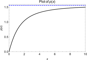
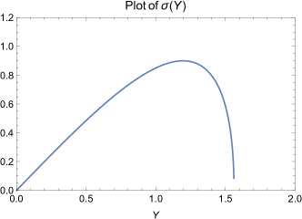
The diffusion in natural scale is bounded between and and is non-explosive. Since the map as , the process in (12) explodes at the first hitting time of to level .
2.3. Nature of Boundary Points
We established above that the process for takes values in the bounded range . The asymptotics of the volatility in the natural scale from Proposition 2.2 determines the nature of the boundary points.
The boundary is similar to that of a geometric Brownian motion process and is a natural boundary.
The point is similar to the origin for the CEV process. Recall the classification of the solutions for this case [29]:
a) . The point is a regular boundary point. The fundamental solution is not unique. The problem is well-posed only if an additional boundary condition is imposed, for example, absorbing or reflecting boundary.
b) . The point is an exit boundary point. There is a unique fundamental solution with decreasing norm and mass at corresponding to the absorption at this point.
2.4. Feller Test of Explosion for the Volatility Process
In this section, we study the explosion for the volatility process in (12). A sufficient condition for the absence of explosions is expressed in terms of the scale function as [26]. By point (i) in Proposition 2.1, the limit of the scale function is finite, so explosions cannot be excluded. However the finiteness of is only a necessary, but not sufficient criterion for the existence of explosions. Using the Feller test of explosion [16], we show in this section that the process in (12) explodes in finite time with non-zero probability.
Proposition 2.3.
The process in (12) explodes in finite time with non-zero probability.
Proof.
Recall the Feller test for explosions of the solutions of a SDE. Define the function
| (34) |
We prove an upper bound on the function , and will show that it is finite for all . Using and the bounds (26) on we have
| (35) |
Recall from (25) that and
| (36) |
Denote the integral
| (37) |
The integrand has the large asymptotics as . This gives the large asymptotics
| (38) |
We distinguish between two cases:
i) . For this case the integral has logarithmic growth as . The bound (35) has the large asymptotics, i.e. there exists some such that
| (39) |
for any sufficiently large , where is given in (27) and the integral is
| (40) |
which is bounded as .
We conclude that for this case for all .
ii) . For this case the integrand in the upper bound (35) on has the large asymptotic form
| (41) |
Consider the two cases of and separately.
a) For the second term in the brackets is and can be neglected for the large asymptotics of the integral. This is with and is thus bounded as .
b) For the second term in the brackets dominates over the first term, and the integrand has the form . The large asymptotics of the integral giving the upper bound on is , which has a finite limit as .
For both cases, the function is bounded from above by a finite value, which implies for all . By the Feller test of explosion (Theorem 2.2), this implies that the process explodes in finite time with non-zero probability. ∎
Remark 2.2.
Since the process for in (12) explodes in finite time with non-zero probability, we have for all . In particular, the expectation is infinite.
3. Capped Volatility Process and VIX Option Pricing
The result of Proposition 2.3 is a surprising negative result. It implies that the VIX futures prices in (4) and VIX call option prices in (5) are infinite, and VIX put option prices in (6) are zero for any maturity and strike . This limits the practical usefulness of the SABR model with for pricing these products.
On the other hand, the SABR model with has well behaved VIX options and futures. The predictions for this case have been discussed in e.g. [17] and [31].
As a remedy for the SABR model with , we propose the cap the drift and diffusion terms in the process to make it non-explosive such that one can price the VIX options in practice. In particular, based on the volatility process in (12), we propose the following modification, the capped volatility process:
| (42) |
with capped volatility and drift
| (43) | |||
| (44) |
where and are given in (13)-(14) and are given caps. Under Assumption 2.1, is monotonically increasing in , and we assume that such that
| (45) |
where
| (46) |
With defined in (42), the asymptotics of the VIX call and put options can be achieved by quoting the results of the short-maturity European call and put options for the local volatility model. First, we will show that almost surely as , and indeed we have the following result.
Proposition 3.1.
For any , we have
| (47) |
Proof.
First, we notice that for any , and . Next, it follows from (42) that for any ,
| (48) |
Therefore, we have
and similarly,
Hence, we conclude that
and
This completes the proof. ∎
Proposition 3.1 implies that almost surely as . We can leverage this result and the short-maturity asymptotics for European options in the local volatility model [6] to obtain the following result for short-maturity asymptotics for OTM VIX options.
Before addressing the short-maturity asymptotics of VIX options we discuss the forward VIX defined as in (4). In the limit this becomes . Due to the explosion of in (12), this expectation is infinite (Remark 2.2). However, the expectation of the capped process gives a finite but -dependent value, which we denote with the capped process given in (42). We prove next a result for the short-maturity limit of at finite .
Proposition 3.2.
We have
| (49) |
Proof.
For any , it follows from (42) that
| (50) |
where and for any . Therefore, we have
| (51) |
and
| (52) |
which completes the proof. ∎
This implies that for sufficiently small , OTM VIX call options have and OTM VIX put options have .
Theorem 3.1.
Let and denote the VIX call and put option prices under the capped volatility model (42). Then
| (53) | |||
| (54) |
where the rate function is
| (55) |
Proof.
By Proposition 3.1 and short-maturity asymptotics for European options in the local volatility model [6], we can compute that for any and ,
where is defined in (55). Similarly, we can compute that for any and ,
Since it holds for any , by letting , we showed that (53) holds. Similarly, we can show that (54) holds. This completes the proof. ∎
In particular, for OTM call options, i.e. , we have
| (56) |
and for OTM put options, i.e. , we have
| (57) |
We define the implied volatility of the VIX options in the capped volatility model (42) as
| (58) | ||||
where and are the undiscounted Black-Scholes option prices with forward and volatility and .
The short-maturity option pricing result of Theorem 3.1 translates in the usual way into a short-maturity result for the VIX implied volatility. Assume that the cap is sufficiently large, such that and . Then, the short-maturity asymptotics for the VIX call and put options is equivalent with the short-maturity asymptotics of the VIX implied volatility
| (59) |
where is the log-strike. We used here the result of Proposition 3.2 to take the limit for any finite .
The integral in the denominator in (59) can be evaluated exactly with the result
| (60) |
The VIX implied volatility (59) can be expanded in log-strike
| (61) |
as , where the ATM level, skew and convexity of the VIX implied volatility are
| (62) | ||||
| (63) |
and
| (64) |
These results for the ATM level, skew and convexity are reproduced by Proposition 6.2 in [31] by taking in that result, although, strictly speaking, they do not follow from Proposition 6.2 of [31] since the CEV local volatility function does not satisfy the technical conditions required for its validity.
Remark 3.1.
For and , the VIX skew (63) is positive, which agrees with the empirical evidence: the observed VIX smile is up-sloping. On the other hand, the VIX convexity (64) is positive, which unfortunately disagrees with empirical evidence: the observed VIX smile is concave. This disfavors the SABR model as a realistic model for VIX smiles.
Numerical simulations. We illustrate the theoretical results with numerical simulations of VIX options under the capped volatility process (42). We assume the following parameters
| (65) |
| 2.336 | ||
| 0.0 | 3.464 | |
| 0.7 | 5.136 |
In Table 1 we show the values of the parameter at which the cap on is reached. For all correlation values, this is much larger than the spot volatility .
The SDE for the capped volatility process in (42) was simulated numerically using an Euler scheme with time steps and MC paths. Table 1 shows the VIX forward prices for for several values of the correlation parameter obtained from the MC simulation. These values are close to .
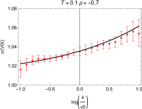
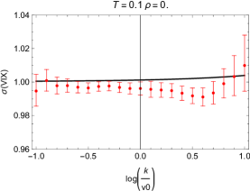
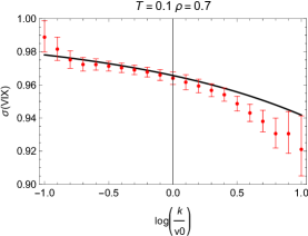
Using this simulation we priced VIX options with maturity . The option prices were converted to VIX implied volatility using the definition (58). The results for are shown in Figure 3.1 as the red dots with error bars, for three values of the correlation . The solid black curve in these plots shows the short-maturity asymptotic VIX volatility (59).
From these plots we note reasonably good agreement of the asymptotic result with the numerical simulation within the errors of the Monte Carlo simulation. These plots also illustrate the main features of the VIX smile under the SABR model noted above: for negative correlation the VIX smile is increasing, which is in agreement with empirical data. However, for the smile is convex, which is different from the observed concave shape of this smile. This suggests that the SABR model may not allow a precise calibration to VIX options market data, although it can be useful as a simple approximation.
Acknowledgements
Lingjiong Zhu is partially supported by the grants NSF DMS-2053454, NSF DMS-2208303.
References
- [1] E. Abi Jaber, C. Illand, and S. Li. The quintic Ornstein-Uhlenbeck volatility model that jointly calibrates SPX and VIX smiles. Risk, June, 2023.
- [2] E. Alós, D. García-Lorite, and A.M. Gonzalez. On smile properties of volatility derivatives: Understanding the VIX skew. SIAM Journal of Financial Mathematics, 13(13):32–69, 2022.
- [3] L. Andersen and J. Andreasen. Volatility skews and extensions of the LIBOR market model. Applied Mathematical Finance, 7(1):1–32, 2000.
- [4] A. Antonov, M. Konikov, and M. Spector. SABR spreads its wings. Risk, August 2013.
- [5] J. Baldeaux and A. Badran. Consistent modelling of VIX and equity derivatives using a 3/2 plus jumps model. Applied Mathematical Finance, 21:299–312, 2014.
- [6] H. Berestycki, J. Busca, and I. Florent. Asymptotics and calibration of local volatility models. Quantitative Finance, 2:61–69, 2002.
- [7] N. Cai, Y. Song, and N. Chen. Exact simulation of the SABR model. Operations Research, 65(4):931–951, 2017.
- [8] H. Cao, A. Badescu, Z. Cui, and S.K. Jayaraman. Valuation of VIX and target volatility options with affine GARCH models. Journal of Futures Markets, 40:1880–1917, 2020.
- [9] P. Carr, H. Geman, D.B. Madan, and M. Yor. Pricing options on realized variance. Finance and Stochastics, 9:453–475, 2005.
- [10] CBOE Global Indices. Volatility Index Methodology: CBOE Volatility Index. White Paper, 2023.
- [11] B. Chen, C.W. Oosterlee, and H. van der Weide. A low-bias simulation scheme for the SABR model. International Journal of Theoretical and Applied Finance, 15(2):125016, 2012.
- [12] R. Constantinescu, N. Costanzino, A.L. Mazzucato, and V. Nistor. Approximate solutions to second order parabolic equations: I. Analytical estimates. Journal of Mathematical Physics, 51:103502, 2010.
- [13] C. Cuchiero, G. Gazzani, J. Möller, and S. Svaluto-Ferro. Joint calibration to SPX and VIX options with signature-based models. To appear in Mathematical Finance, 2025.
- [14] Z. Cui, J. Kirkby, and D. Nguyen. Efficient simulation of generalized SABR and stochastic local volatility models. European Journal of Operational Research, 290(3):1046–1062, 2021.
- [15] J. Detemple and C. Osakwe. The valuation of volatility options. European Finance Review, 4:21–50, 2000.
- [16] W. Feller. The parabolic differential equations and the associated semi-groups of transformations. Annals of Mathematics, 55(3):468–519, 1952.
- [17] M. Forde and B. Smith. Markovian stochastic volatility with stochastic correlation - joint calibration and consistency of SPX/VIX short-maturity smiles. International Journal of Theoretical and Applied Finance, 2-3:2350007, 2023.
- [18] J. Goard and M. Mazur. Stochastic volatility models and the pricing of VIX options. Mathematical Finance, 23:439–458, 2013.
- [19] O. Grishchenko, X. Han, and V. Nistor. A volatility-of-volatility expansion of the option prices in the SABR stochastic volatility model. International Journal of Theoretical and Applied Finance, 23(3):2050018, 2020.
- [20] J. Guyon. The joint SP500/VIX smile calibration puzzle solved. Risk, June, 2020.
- [21] J. Guyon. Dispersion-constrained martingale Schrödinger problems and the exact join S&P500/VIX smile calibration puzzle. Finance and Stochastics, 28:27–79, 2024.
- [22] P.S. Hagan, D. Kumar, A.S. Lesniewski, and D.E. Woodward. Managing smile risk. Wilmott Magazine, September 2002.
- [23] P. Henry-Labordère. Analysis, Geometry and Modeling in Finance. Advanced Methods in Option Pricing. Chapman and Hall/CRC, 2008.
- [24] J. Hull and A. White. The pricing of options on assets with stochastic volatilities. Journal of Finance, 42(2):281–300, 1987.
- [25] O. Islah. Solving SABR in exact form and unifying it with LIBOR market model. SSRN, 1489428, 2009.
- [26] I. Karatzas and S. Shreve. Brownian Motion and Stochastic Calculus. Springer Verlag, 2nd edition, 1991.
- [27] A.L. Lewis. Option Valuation Under Stochastic Volatility. Finance Press, 2000.
- [28] A.L. Lewis. Option Valuation Under Stochastic Volatility II. Finance Press, 2016.
- [29] V. Linetsky and R. Mendoza. The constant elasticity of variance model. In R. Cont, editor, Encyclopedia of Quantitative Finance. John Wiley and Sons, 2010.
- [30] P.L. Lions and M. Musiela. Correlations and bounds for stochastic volatility models. Annales de l’Institut Henri Poincare C, Analyse non lineaire, 24:1–16, 2007.
- [31] D. Pirjol, X. Wang, and L. Zhu. Short-maturity asymptotics for VIX and European options in local-stochastic volatility models. arxiv:2407.16813[q-fin], 2024.
- [32] A. Sepp. Pricing options on realized variance in Heston model with jumps in returns. Journal of Computational Finance, 11:33–70, 2008.
- [33] A. Sepp. VIX option pricing in a jump-diffusion model. Risk, May:84–89, 2008.
- [34] C. Tong and Z. Huang. Pricing VIX options with realized volatility. Journal of Future Markets, 41(8):118–1200, 2021.
- [35] P. Yuan. Time-varying skew in VIX derivatives pricing. Management Science, 68(10):7065–7791, 2022.