Dynamics of “Spontaneous” Topic Changes in Next Token Prediction with Self-Attention

Abstract

Human cognition can spontaneously shift conversation topics, often triggered by emotional or contextual signals. In contrast, self-attention-based language models depend on structured statistical cues from input tokens for next-token prediction, lacking this spontaneity. Motivated by this distinction, we investigate the factors that influence the next-token prediction to change the topic of the input sequence. We define concepts of topic continuity, ambiguous sequences, and change of topic, based on defining a topic as a set of token priority graphs (TPGs). Using a simplified single-layer self-attention architecture, we derive analytical characterizations of topic changes. Specifically, we demonstrate that (1) the model maintains the priority order of tokens related to the input topic, (2) a topic change can occur only if lower-priority tokens outnumber all higher-priority tokens of the input topic, and (3) unlike human cognition, longer context lengths and overlapping topics reduce the likelihood of spontaneous redirection. These insights highlight differences between human cognition and self-attention-based models in navigating topic changes and underscore the challenges in designing conversational AI capable of handling “spontaneous” conversations more naturally. To the best of our knowledge, no prior work has explored these questions with a focus as closely aligned to human conversation and thought.

1 Introduction

In human cognition, topic changes often occur sporadically, with little apparent structure or forethought: an spontaneous shift in focus during a conversation, a sudden leap between ideas when brainstorming, or an unexpected redirection in storytelling. These seemingly chaotic shifts are intrinsic to the human way of processing and communicating information (Christoff and Fox,, 2018; Mills et al.,, 2020). For instance, someone discussing their favorite book might suddenly mention a family gathering. This abrupt change may be due to an emotional connection, such as recalling reading that book during a family vacation, where sensory details like the scent of the ocean or the warmth of the sun trigger a vivid memory. The hippocampus helps link these sensory cues to memories, enabling a meaningful shift (Lisman et al.,, 2017). The prefrontal cortex then integrates these memories, emotions, and context to redirect conversations spontaneously (Miller and Cohen,, 2001).

However, large language models (LLMs) rely on contextual signals in the input to perform topic shifts. Unlike humans, who transition intuitively between topics, often driven by emotion or creativity, LLMs follow a structured, statistical approach, remaining on topic unless explicit cues signal a change. Figure 2 illustrates this distinction using the first sentence of the book “One hundred years of solitude” (García Márquez,, 1967). Additionally, related studies on conversational agents have recognized the practical challenges of spontaneous topic changes and proposed various practical approaches (Lim et al.,, 2010; Hwang et al.,, 2024; Xie et al.,, 2021; Soni et al.,, 2022; Ni et al.,, 2022; Lin et al.,, 2023).

It is also important to differentiate between topic changes and hallucinations. Hallucinations involve generating incorrect or fabricated information without clear contextual basis, often resulting in false or illogical content (Ji et al.,, 2023; Maynez et al.,, 2020). In contrast to topic changes, hallucinations are not deliberate or contextually driven shifts in discourse. More interestingly, some hallucinations may still appear to maintain topic consistency by staying loosely connected to the previous topic, yet they fail to introduce a meaningful or valid change. Our focus is on understanding when and why self-attention models predict next tokens from a different topic of the input, examining the conditions under which an input sequence from one topic leads to a prediction in another.

Recent advancements in the related field have substantially deepened our understanding of self-attention mechanisms in LLMs. The Transformer model, introduced by Vaswani et al., (2017), revolutionized natural language processing by using self-attention to determine the importance of each token in relation to others. This innovation enables Transformers to focus on relevant context when predicting the next token, significantly enhancing capabilities natural language understanding and generation(Brown et al.,, 2020; Clark et al.,, 2019; Devlin et al.,, 2019; Bisk et al.,, 2020). Additionally, connections between self-attention and support vector machines (SVMs) have offered valuable insights into optimization strategies, and mechanisms within the next token prediction (Tarzanagh et al., 2023b, ; Tarzanagh et al., 2023a, ; Li et al., 2024b, ). These advancements underscore the transformative role of attention-based architectures in token prediction tasks. A recent study by Li et al., (2023) highlights that in mixed topic inputs, transformers achieve higher pairwise attention between same-topic words compared to different-topic words. However, our approach aligns more closely with human cognitive processes, where the input is typically centered on a single topic, ensuring that discussions or conversations remain within a consistent context or theme.

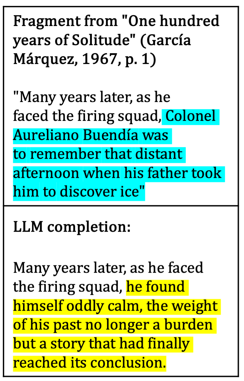
Figure 1: Illustration of the difference between human cognition and AI contextual completion. The original fragment of “One hundred years of solitude" (García Márquez,, 1967) (top) has a clear “spontaneous" thought, but the GPT-2’s completion (bottom), demonstrates continuity.

Despite these advancements, our understanding of how LLMs manage topic changes compared to human cognition remains limited. Human cognition seamlessly navigates such transitions through spontaneous thought and contextual awareness (Christoff and Fox,, 2018). Investigating this distinction could provide valuable insights into the strengths and limitations of language models in mimicking human-like conversation. Bridging this gap is essential for enhancing language models, particularly in their ability to adapt to and manage dynamic topic changes–a process closely aligned with the flow of spontaneous thought in human cognition. Specifically, we address the following research questions:

• What underlying mechanism drives topic changes during next token prediction in self-attention architectures?

• Which factors shape the dynamics of topic changes in next token prediction?

To answer the above questions, it is essential first to explore how self-attention allocates attention to tokens for next token prediction with respect to the input topic. Understanding how attention weights are allocated offers key insights into the prioritization of tokens by self-attention mechanisms, particularly when models are trained on datasets spanning multiple topics. This fundamental understanding will pave the way for uncovering the role of attention patterns in driving “spontaneous” topic changes. To the best of our knowledge, there are no other studies that have investigated these dynamics so closely in relation to human conversation and thought processes.

Summary of Findings

For simplicity, we elaborate our results using a two-topic scenario, but it is straightforward to extend them to multiple topics. Imagine an oracle that is an expert on Topic A, capable of following any conversation within that topic while staying true to its context. Now, suppose the oracle gains knowledge of Topic B and is following a conversation about Topic A. Will the oracle’s responses remain firmly within Topic A, or will the influence of the knowledge of Topic B cause the conversation to drift? This analogy encapsulates the problem we address: understanding when and why attention models might preserve a topic or change to another “spontaneously". Specifically, we make the following contributions:

1. Preservation of input topic priorities. Using a controlled sandbox, we demonstrate in Theorem 3 that attention models trained on mixed-topic datasets maintain the priorities of tokens associated with the original topic of an input sequence (Topic A in our analogy).

2. Changing topics triggered by token frequency. In Theorem 4, we show that only if a lower-priority token appears more frequently than all higher-priority tokens of Topic A, the oracle’s responses may reflect a change of topic.

3. Impact of sequence length and topic overlap. Theorem 5 establishes that longer input sequences decrease the likelihood of changing topics. Furthermore, overlapping topics act as a stabilizing factor, not increasing the frequency of “spontaneous” topic changes. This finding represents a key contribution to the development of human-like AI conversational models. Unlike human dialogue, where extended discussions often encourage spontaneous topic shifts and overlapping topics promote cognitive connections that facilitate smooth transitions, our results highlight a fundamental limitation of attention-based models in replicating these human-like dynamics.

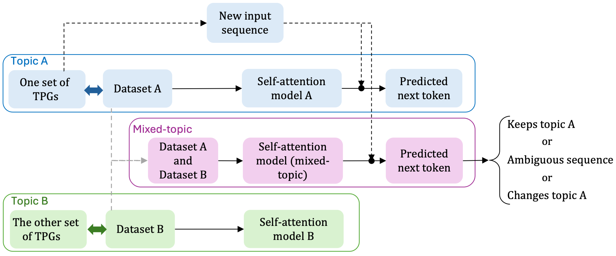
Figure 2: Overview of our approach. We define a topic by a set of TPGs $\{\mathcal{G}^{(k)}\}^{K}_{k=1}$ (Def. 2) and generate a dataset for each topic such that the dataset can reconstruct the corresponding TPGs exactly (Assumption 4). The combination of dataset A and dataset B becomes the dataset for the mixed-topic model. We train self-attention models independently on each dataset. Then, we generate a new input sequence from topic A and predict the next token with two models, self-attention model A and self-attention model (mixed-topic). The next-token prediction with the mixed-topic model is categorized into three outcomes: keeps topic A (topic continuity from Def. 3), ambiguous sequence (from Def. 4), changes topic A (change of topic from Def. 5). Further details for each category are in Figure 4.

Following the framework of token-priority graphs (TPGs) introduced by Li et al., 2024b , we start with defining a topic as a set of TPGs (see Sec 3). For simplicity, we consider two different topics, Topic A and Topic B, characterized by two different sets of TPGs. We demonstrate the preservation of input topic priorities in a model trained with mixed-topic datasets (see Sec 4). Additionally, we introduce three concepts to categorize the prediction outputs: topic continuity, ambiguous sequence, and change of topic. Figure 2 outlines the structural overview of our approach. We subsequently establish the conditions under which a self-attention model induces a topic change, showing that the probability of topic changes does not increase with longer input sequences or the presence of overlapping topics (see Sec 5). All proofs are refer to Appendix A. To formalize this approach, we begin with the structured problem setup.

2 Problem Setup

Next Topic Prediction with Self-attention Model

In line with the approach presented by Tarzanagh et al., 2023b and Li et al., 2024b , we frame the next-token prediction task as a multi-class classification problem. Given a vocabulary of size $K$ with an embedding matrix ${\bf E}=[{\bf e}_{1}\ {\bf e}_{2}\ \cdots\ {\bf e}_{K}]^{\top}\in\mathbb{R}^{K\times d}$, we aim to predict the next token ID $y\in[K]$ based on an input sequence ${\bf X}=[{\bf x}_{1}\ {\bf x}_{2}\ \cdots\ {\bf x}_{T}]^{\top}\in\mathbb{R}^{T\times d}$ with ${\bf x}_{i}\in{\bf E}$ for all $i\in[T]$. The training dataset, denoted as

$$\text{DSET}=\{({\bf X}_{i},y_{i})\in\mathbb{R}^{T_{i}\times d}\times[K]\}_{i=1}^{n},$$

contains sequences of varying lengths $T_{i}$. In our notation ${\bf x}$ is the embedding vector corresponding to the token ID $x$, this is ${\bf x}={\bf e}_{x}$. For prediction, we utilize a single-layer self-attention model with a combined key-query weight matrix ${\bf W}\in\mathbb{R}^{d\times d}$ and identity value matrix as in Tarzanagh et al., 2023b . The self-attention embedding output

$$f_{\bf W}({\bf X})={\bf X}^{\top}\mathbb{S}({\bf X}{\bf W}\bar{{\bf x}}),$$ (output)

where $\mathbb{S}(\cdot)$ is the softmax operation and $\bar{{\bf x}}:={\bf x}_{T}$, serves as a weighted representation of the tokens, allowing for context-sensitive prediction of $y$ based on the final input token. Let $\ell:\mathbb{R}\to\mathbb{R}$ be a loss function. For the training dataset DSET, we consider the empirical risk minimization (ERM) with:

$$L({\bf W})=\frac{1}{n}\sum_{i=1}^{n}\ell({\bf c}_{y_{i}}^{\top}{\bf X}_{i}^{\top}\mathbb{S}({\bf X}_{i}{\bf W}\bar{{\bf x}}_{i})).$$ (ERM)

We assume a well pre-trained classification head matrix ${\bf C}=[{\bf c}_{1}\ {\bf c}_{2}\ \cdots\ {\bf c}_{K}]^{\top}\in\mathbb{R}^{K\times d}$. Each classification head ${\bf c}_{k}\in\mathbb{R}^{d}$ is fixed and bounded for all $k\in[K]$. Starting from ${\bf W}^{(0)}\in\mathbb{R}^{d\times d}$ with step size $\eta>0$, for $\tau\geq 0$ we optimize ${\bf W}$ with a gradient descent algorithm

$${\bf W}^{(\tau+1)}={\bf W}^{(\tau)}-\eta\nabla L({\bf W}^{(\tau)}).$$ (Algo-GD)

We keep the first two assumptions from Li et al., 2024b :

Assumption 1.

$\forall y,k\in[K],k\neq y,{\bf c}_{y}^{\top}{\bf e}_{y}=1$ and ${\bf c}_{y}^{\top}{\bf e}_{k}=0$

Assumption 2.

For any $({\bf X},y)\in\text{DSET}$, the token ${\bf e}_{y}$ is contained in the input sequence ${\bf X}$.

Assumption 1 represents a variation of the weight-tying approach commonly used in language models (Press and Wolf,, 2017; Vaswani et al.,, 2017). Once training is complete, for a new input sequence ${\bf X}$, and a model characterized by $\bf W$, we predict the next token ID $\hat{y}_{\bf w}$ based on greedy decoding the probabilities from the softmax of the classification output

$$\hat{y}_{\bf w}\in\arg\max_{k\in[K]}\left[\mathbb{S}\left({\bf C}f_{\bf W}({\bf X})\right)\right]_{k}.$$ (1)

Token-priority Graph and Global Convergence of the Self-attention Model

Li et al., 2024b defined a token-priority graph (TPG) as a directed graph with nodes representing tokens in the vocabulary. $\text{DSET}^{(k)}$ is a subset of sequences from DSET with the same last token is ${\bf e}_{k}=\bar{\bf x}$. They defined TPGs $\{\mathcal{G}^{(k)}\}_{k=1}^{K}$ such that every $\mathcal{G}^{(k)}$ is a directed graph where for every sequence $({\bf X},y)\in\text{DSET}^{(k)}$ a directed edge is added from ${\bf e}_{y}$ to every token ${\bf x}\in{\bf X}$. TPGs are further divided into strongly-connected components (SCCs), which capture subsets of tokens where priority relations are cyclic, indicating comparable token importance. For tokens within two different SCCs, strict priority orders emerge, helping the model to differentiate between tokens when learning next-token predictions. We use the same notation as Li et al., 2024b , given a directed graph $\mathcal{G}$, for $i,j\in[K]$ such that $i\neq j$:

• $i\in\mathcal{G}$ denotes that the node $i$ belongs to $\mathcal{G}$.

• $(i\Rightarrow j)\in\mathcal{G}$ denotes that the directed path $(i\rightarrow j)$ is present in $\mathcal{G}$ but $j\rightarrow i$ is not.

• $(i\asymp j)\in\mathcal{G}$ means that both nodes $i$ and $j$ are in the same strongly connected component (SCC) of $\mathcal{G}$ (there exists both a path $i\rightarrow j$ and $j\rightarrow i$).

For any two distinct nodes $i,j$ in the same TPG, they either satisfy $(i\Rightarrow j)$, $(j\Rightarrow i)$ or $(i\asymp j)$. Nodes in each $\mathcal{G}^{(k)}$ represent indices in $[K]$, and SCC structure supports the self-attention mechanism’s ability to assign priority within sequences based on the conditioning last token. Theorem 2 of Li et al., 2024b proved that under Assumptions 1 and 2, the self-attention model learned through Algo-GD converges to the solution of the following Support Vector Machine (SVM) defined by the TPGs of the underlying dataset DSET

$${\bf W}^{\text{svm}}=\arg\min_{\bf W}\|{\bf W}\|_{F}$$ (Graph-SVM)

$$\text{s.t.}\quad({\bf e}_{i}-{\bf e}_{j})^{\top}{\bf W}{\bf e}_{k}\begin{cases}=0,&\forall(i\asymp j)\in\mathcal{G}^{(k)}\\ \geq 1,&\forall(i\Rightarrow j)\in\mathcal{G}^{(k)}\end{cases}\forall k\in[K].$$

Here is a condensed version of the theorem:

Theorem 1 (Li et al., 2024b ).

Consider dataset DSET and suppose Assumptions 1 and 2 hold. Set loss function as $\ell(u)=-\log(u)$. Starting Algo-GD from any ${\bf W}(0)$ with constant size $\eta$, if ${\bf W}^{\text{svm}}\neq{\bf 0}$,

$$\tilde{\bf W}=\lim_{\tau\to\infty}\frac{{\bf W}(\tau)}{\|{\bf W}(\tau)\|_{F}}=\frac{{\bf W}^{\text{svm}}}{\|{\bf W}^{\text{svm}}\|_{F}}$$ (2)

This convergence implies that the model predicts the next token based on priorities obtained from the SCCs within the TPG relevant to the last token of the input sequence. Unlike the work in Li et al., 2024b , which considers multiple loss functions in subsequent results, we focus exclusively on a log-loss function in this work, leaving the exploration of other loss functions for future research. We add here another reasonable assumption that prevents the probabilities in Equation 1 to be equal for improbable numerical reasons, and we present our first lemma.

Assumption 3.

For any $({\bf X},y)\in\text{DSET}$, $\exists i,j\in[T]\text{ and }u,v\in\mathbb{Z}$ such that $u\left[\mathbb{S}({\bf X}\tilde{\bf W}\bar{{\bf x}})\right]_{i}=v\left[\mathbb{S}({\bf X}{\tilde{\bf W}}\bar{{\bf x}})\right]_{j}\text{ if and only if }u=v\text{ and }\left[\mathbb{S}({\bf X}\tilde{\bf W}\bar{{\bf x}})\right]_{i}=\left[\mathbb{S}({\bf X}{\tilde{\bf W}}\bar{{\bf x}})\right]_{j}$.

Lemma 2.

Suppose conditions from Theorem 1 and Assumption 3 hold. Consider an input sequence ${\bf X}$ from DSET^(k) and corresponding TPG $\mathcal{G}^{(k)}$, $\forall i,j\in[K]$ we have $\left[\mathbb{S}\left({\bf C}f_{\bf W}({\bf X})\right)\right]_{i}=\left[\mathbb{S}\left({\bf C}f_{\tilde{\bf W}}({\bf X})\right)\right]_{j}\text{ iff }(x_{i}\asymp x_{j})\in\mathcal{G}^{(k)}$.

This means that the tokens that maximize the probability in Equation 1 are all within the same SCC leading to the following definition:

Definition 1 (highest probability SCC).

Consider an input sequence ${\bf X}$ from DSET^(k) and corresponding TPG $\mathcal{G}^{(k)}$. We define $\widehat{\mathcal{G}}^{(k)}({\bf X})\in\mathcal{G}^{(k)}$ as the highest probability SCC for ${\bf X}$ in $\mathcal{G}^{(k)}$ such that $\forall{\bf x}\in\widehat{\mathcal{G}}^{(k)}({\bf X})$ we have $\left[\mathbb{S}\left({\bf C}f_{\tilde{\bf W}}({\bf X})\right)\right]_{x}=\left\|\mathbb{S}\left({\bf C}f_{\tilde{\bf W}}({\bf X})\right)\right\|_{\infty}$.

3 Defining Topics

In order to answer our research questions regarding the dynamics of topic changes we need to define the concept of a topic. In the previous settings, a dataset DSET generates TPGs $\{\mathcal{G}^{(k)}\}_{k=1}^{K}$, but, conversely, an existing set of TPGs can generate DSET, akin to generating data from a particular topic, which leads to the following definitions.

Definition 2 (topic).

A topic $\mathbb{T}$ is a set of TPGs $\{\mathcal{G}^{(k)}\}_{k=1}^{K}$. Given topic $\mathbb{T}$ defined by TPGs $\{\mathcal{G}^{(k)}\}_{k=1}^{K}$, input sequence ${\bf X}$ belongs to $\mathbb{T}$ if $\forall{\bf x}\in{\bf X},x\in\mathcal{G}^{(\bar{x})}$. A sequence $({\bf X},y)$ is within $\mathbb{T}$ if ${\bf X}$ belongs to $\mathbb{T}$ and $\forall{\bf x}\in{\bf X},\ (y\Rightarrow x)\in\mathcal{G}^{(\bar{x})}$.

We can define a topic as a set of TPGs because it inherently captures the relationships and contextual dependencies between tokens, offering a structured representation of a topic’s semantics. This means that we can use a topic $\mathbb{T}$ to generate DSET by sampling sequences $({\bf X},y)$ within $\mathbb{T}$. Given the finite number of edges, a DSET can be generated from $\mathbb{T}$ such that it can reconstruct the exact TPGs $\{\mathcal{G}^{(k)}\}_{k=1}^{K}$ that define $\mathbb{T}$, following the construction method in Li et al., 2024b . This leads to the following reasonable assumption:

Assumption 4.

A DSET generated from any topic $\mathbb{T}$ defined by $\{\mathcal{G}^{(k)}\}_{k=1}^{K}$ exactly reconstructs back the TPGs $\{\mathcal{G}^{(k)}\}_{k=1}^{K}$.

Detailed explanation is provided in Appendix B. This assumption enables the application of the results from Li et al., 2024b , with the concepts of topics and TPGs being used interchangeably.

Definition 3 (topic continuity).

Given an input sequence ${\bf X}$ that belongs to $\mathbb{T}$, a weight matrix ${\bf W}$ is said to keep topic $\mathbb{T}$ for the input sequence ${\bf X}$ if $\hat{y}_{\bf W}\in\widehat{\mathcal{G}}^{(k)}({\bf X})$.

This definition establishes the criteria for a next predicted token to preserve the topic of the input sequence. Notice that if we have two topics, $\mathbb{T}_{a}$ and $\mathbb{T}_{b}$, we can generate two different datasets DSET_a and DSET_b. It is clear that $\tilde{\bf W}_{a}$ trained only with DSET_a will always keep topic $\mathbb{T}_{a}$. But we could also obtain $\tilde{\bf W}_{ab}$ with a dataset combining DSET_a and DSET_b as training sets. The central question is whether $\tilde{\bf W}_{ab}$ keeps topic $\mathbb{T}_{a}$, given an input sequence ${\bf X}$ that belongs to $\mathbb{T}_{a}$, or if it instead predicts tokens that prompt a topic change. This can be understood through an analogy: consider an oracle only proficient in Topic A, capable of following conversations in the context of Topic A. If this oracle gains knowledge of Topic B, will it continue to follow the conversation within Topic A’s context when the conversation is within Topic A, or will its response begin to exhibit a shift to Topic B?

4 Attention within Mixed Topics

Let’s first understand the way in which attention models assign priority to tokens within mixed-topic setting. For simplicity, we elaborate our results using a two-topic scenario, but it is straightforward to extend all of our theoretical results on multiple topics. Notice the self-attention embedding output is a linear combination of $\bf X$ given by $\mathbb{S}({\bf XW\bar{x}})$. The embeddings in $\bf X$ corresponding to the highest entries in the vector $\mathbb{S}({\bf XW\bar{x}})$ will receive higher priority in their importance to predict the next token, therefore we can hypothesize that models in which $\mathbb{S}({\bf XW\bar{x}})$ are ordered in a similar way will predict similar next tokens. This idea leads to our first main result which considers this situation within a mixed topics setting:

Theorem 3.

Consider datasets DSET_a and DSET_b from topics $\mathbb{T}_{a}$ and $\mathbb{T}_{b}$, respectively. Let DSET_ab be the union of DSET_a and DSET_b. Suppose Assumptions 1, 2, 3 and 4 hold. Set loss function as $\ell(u)=-\log(u)$. Starting Algo-GD from any initial point with constant size $\eta$ and if ${\bf W}_{a}^{\text{svm}}\neq{\bf 0}$ and ${\bf W}_{ab}^{\text{svm}}\neq{\bf 0}$; for a given sequence ${\bf X}$ that belongs to $\mathbb{T}_{a}$, we have that $\tilde{\bf W}_{ab}$ preserves the attention priority of $\mathbb{T}_{a}$ on input ${\bf X}$. This is $\forall i,j\in[T]$:

• $\text{if }\quad[\mathbb{S}({\bf X}\tilde{\bf W}_{a}\bar{{\bf x}})]_{i}=[\mathbb{S}({\bf X}\tilde{\bf W}_{a}\bar{{\bf x}})]_{j}\text{ then }\\ \quad[\mathbb{S}({\bf X}\tilde{\bf W}_{ab}\bar{{\bf x}})]_{i}=[\mathbb{S}({\bf X}\tilde{\bf W}_{ab}\bar{{\bf x}})]_{j}$

• $\text{if }\quad[\mathbb{S}({\bf X}\tilde{\bf W}_{a}\bar{{\bf x}})]_{i}>[\mathbb{S}({\bf X}\tilde{\bf W}_{a}\bar{{\bf x}})]_{j}\text{ then }\\ \quad[\mathbb{S}({\bf X}\tilde{\bf W}_{ab}\bar{{\bf x}})]_{i}\geq[\mathbb{S}({\bf X}\tilde{\bf W}_{ab}\bar{{\bf x}})]_{j}$

• $\text{if }\quad[\mathbb{S}({\bf X}\tilde{\bf W}_{a}\bar{{\bf x}})]_{i}<[\mathbb{S}({\bf X}\tilde{\bf W}_{a}\bar{{\bf x}})]_{j}\text{ then }\\ \quad[\mathbb{S}({\bf X}\tilde{\bf W}_{ab}\bar{{\bf x}})]_{i}\leq[\mathbb{S}({\bf X}\tilde{\bf W}_{ab}\bar{{\bf x}})]_{j}$

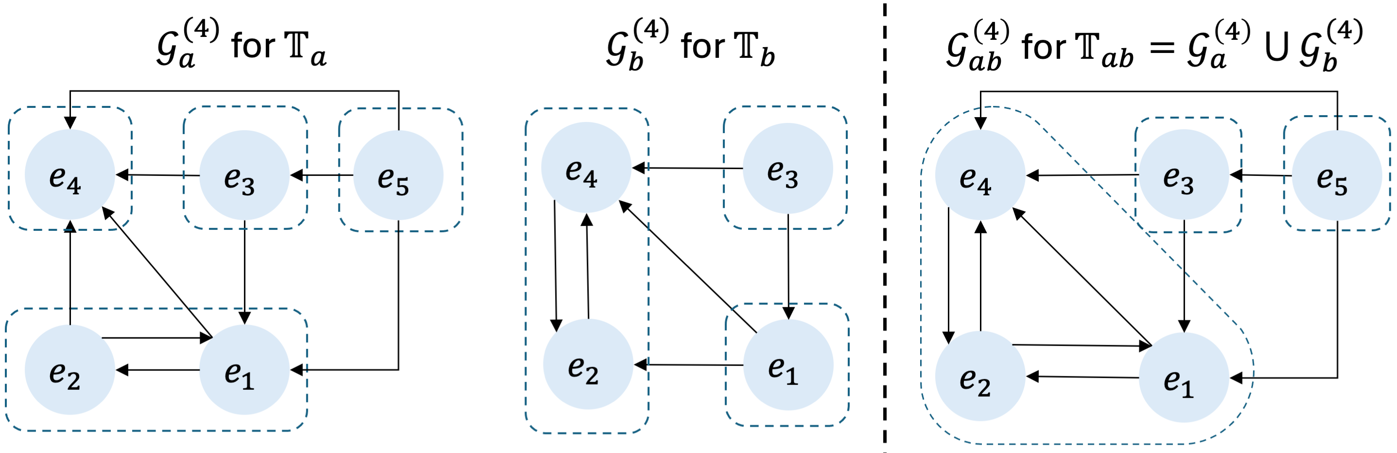
Figure 3: Illustration of topic combination. $\mathcal{G}^{(4)}_{a}$ and $\mathcal{G}^{(4)}_{b}$ are token-priority graphs (TPGs) of the last token ${\bf e}_{4}$ for $\mathbb{T}_{a}$ and $\mathbb{T}_{b}$, respectively. $\mathcal{G}^{(4)}_{ab}$ combines the TPG for $\mathbb{T}_{a}$ and the TPG for $\mathbb{T}_{b}$.

This implies that for an input sequence $\mathbf{X}$, a model trained in a mixed-topic setting will maintain the priority of the topic to which $\mathbf{X}$ belongs. Consequently, the attention will be allocated in the same order as if the model had been trained exclusively on the original topic of $\mathbf{X}$. The input sequence ${\bf X}=[{\bf e}_{5},{\bf e}_{1},{\bf e}_{3},{\bf e}_{4}]^{\top}$, as shown in Figure 4 (top), is generated from $\mathbb{T}_{a}$. The predicted next token $\hat{y}_{{\bf w}_{ab}}$ is ${\bf e}_{5}$ and the highest probability SCC in mixed-topics is $\widehat{\mathcal{G}}^{(4)}_{ab}({\bf X})=\{{\bf e}_{5}\}$. Since $\hat{y}_{{\bf w}_{ab}}$ belongs to ${\widehat{\mathcal{G}}}^{(4)}_{ab}({\bf X})$, ${\bf W}_{ab}$ for input sequence $\bf X$ is considered as topic continuity, based on the Definition 3.

The only assumption about ${\bf X}$ on Theorem 3 is that it belongs to $\mathbb{T}_{a}$. However, if $\mathbf{X}$ belongs to $\mathbb{T}_{a}$ and $\mathbb{T}_{b}$, the priority will be preserved within both topics. Additionally, strict equality in the attention priority is maintained, but strict inequalities may not be when combining both datasets. In such cases, the union of their TPGs can form new SCCs, disrupting strict priority. As illustrated in Figure 3, we present $\mathcal{G}^{(4)}_{a}$ and $\mathcal{G}^{(4)}_{b}$ as the TPGs corresponding to last input token ${\bf e}_{4}$ for $\mathbb{T}_{a}$ and $\mathbb{T}_{b}$, respectively. In $\mathcal{G}^{(4)}_{a}$, the token priority is ${\bf e}_{5}>{\bf e}_{3}>{\bf e}_{1}={\bf e}_{2}>{\bf e}_{4}$. Once combining $\mathcal{G}^{(4)}_{a}$ and $\mathcal{G}^{(4)}_{b}$, the priority order in the mixed-topics is ${\bf e}_{5}>{\bf e}_{3}>{\bf e}_{1}={\bf e}_{2}={\bf e}_{4}$, based on $\mathcal{G}^{(4)}_{ab}$. The strict equality ${\bf e}_{1}={\bf e}_{2}$ from $\mathcal{G}^{(4)}_{a}$ is maintained in $\mathcal{G}^{(4)}_{ab}$, but the strict inequality ${\bf e}_{2}>{\bf e}_{4}$ is replaced with ${\bf e}_{2}={\bf e}_{4}$ in mixed-topics, forming the new SCC, $\{{\bf e}_{1},{\bf e}_{2},{\bf e}_{4}\}$, in $\mathcal{G}^{(4)}_{ab}$.

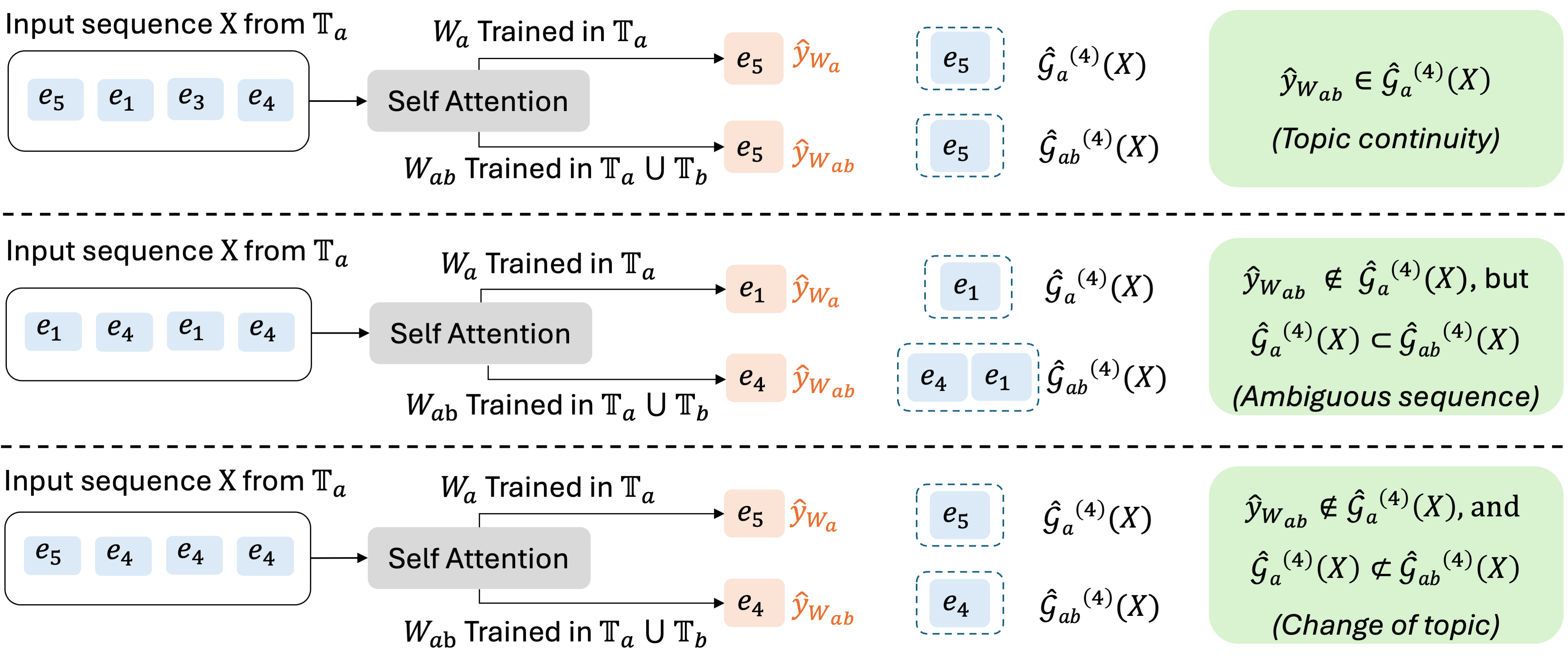
Figure 4: Illustration of topic continuity, ambiguous sequence, and change of topic (see Definition 3,  4, and 5 for formal definitions). For each input sequence derived from $\mathbb{T}_{a}$, we employ a self-attention model trained on $\mathbb{T}_{a}$ and another model trained on the mixed-topics dataset $\mathbb{T}_{ab}$ to predict the next tokens $\hat{y}_{{\bf w}_{a}}$ and $\hat{y}_{{\bf w}_{ab}}$, respectively (orange). $\widehat{\mathcal{G}}^{(4)}_{ab}$ is the highest probability SCC (see Definition 1) in mixed-topics setting and $\widehat{\mathcal{G}}^{(4)}_{a}$ is the highest probability SCC in $\mathbb{T}_{a}$. Top: The input sequence is classified as topic continuity if $\hat{y}_{{\bf w}_{ab}}\in\widehat{\mathcal{G}}^{(4)}_{a}(X)$. Middle: The input sequence is ambiguous if $\hat{y}_{{\bf w}_{ab}}\not\in\widehat{\mathcal{G}}^{(4)}_{a}(X)$, but $\widehat{\mathcal{G}}^{(4)}_{a}(X)\subset\widehat{\mathcal{G}}^{(4)}_{ab}(X)$. Bottom: ${\bf W}_{ab}$ is considered to change of topic, if $\hat{y}_{{\bf w}_{ab}}\not\in\widehat{\mathcal{G}}^{(4)}_{a}(X)$ and $\widehat{\mathcal{G}}^{(4)}_{a}(X)\not\subset\widehat{\mathcal{G}}^{(4)}_{ab}(X)$. The numeric details are provided in Appendix C.3.

To further illustrate Theorem 3 we define the attention priority similarity of weights ${\bf W}^{\prime}$ relative to ${\bf W}$ for a sequence ${\bf X}$ as: $R_{{\bf W},{\bf W}^{\prime}}({\bf X})=$

$$\frac{1}{T-1}\sum_{j=1}^{T-1}g\left(\left[\mathbb{S}\left({\bf X}{\bf W}^{\prime}\bar{\bf x}\right)\right]_{i_{j}}-\left[\mathbb{S}\left({\bf X}{\bf W}^{\prime}\bar{\bf x}\right)\right]_{i_{j+1}}\right),$$

where $i_{1},\cdots,i_{T}$ is a permutation of $1,\cdots,T$ such that $\left[\mathbb{S}\left({\bf X}{\bf W}\bar{\bf x}\right)\right]_{i_{1}}\geq\cdots\geq\left[\mathbb{S}\left({\bf X}{\bf W}\bar{\bf x}\right)\right]_{i_{T}}$, and

$$g(w)=\begin{cases}1,&\text{if $w\geq 0$,}\\ \frac{1}{e^{-w}},&\text{otherwise.}\end{cases}$$

The attention priority similarity quantifies how well the weights ${\bf W}^{\prime}$ preserve the attention priority of the weights ${\bf W}$. A value of 1 indicates that the priority is fully preserved. Using this metric, we conduct experiments, with results in Figure 5. We generate embeddings with $K=10$ and $d=16$, and randomly construct TPGs for $\mathbb{T}_{a}$ and $\mathbb{T}_{b}$. Using these TPGs, we randomly generate $\text{DSET}_{a}$ and $\text{DSET}_{b}$. We compute $\frac{{\bf W}_{a}(\tau)}{\|{\bf W}_{a}(\tau)\|_{F}}$, $\frac{{\bf W}_{b}(\tau)}{\|{\bf W}_{b}(\tau)\|_{F}}$ and $\frac{{\bf W}_{ab}(\tau)}{\|{\bf W}_{ab}(\tau)\|_{F}}$ using the same procedure as Li et al., 2024b . We generate test sequences ${\bf Z}$ within $\mathbb{T}_{a}$, and we calculate the attention priority similarity of $\frac{{\bf W}_{ab}(\tau)}{\|{\bf W}_{ab}(\tau)\|_{F}}$ relative to both $\frac{{\bf W}_{a}(\tau)}{\|{\bf W}_{a}(\tau)\|_{F}}$ and $\frac{{\bf W}_{b}(\tau)}{\|{\bf W}_{b}(\tau)\|_{F}}$. We repeat this process for multiple TPGs and input sequences (simulation details in Appendix C). Figure 5 clearly demonstrates that the similarity converges to 1 after $\tau=8000$ iterations when evaluated relative to $\frac{{\bf W}_{a}(\tau)}{\|{\bf W}_{a}(\tau)\|_{F}}$ (blue line), but fails to converge relative to $\frac{{\bf W}_{b}(\tau)}{\|{\bf W}_{b}(\tau)\|_{F}}$ (orange line). These observations align with the results of Theorem 3.

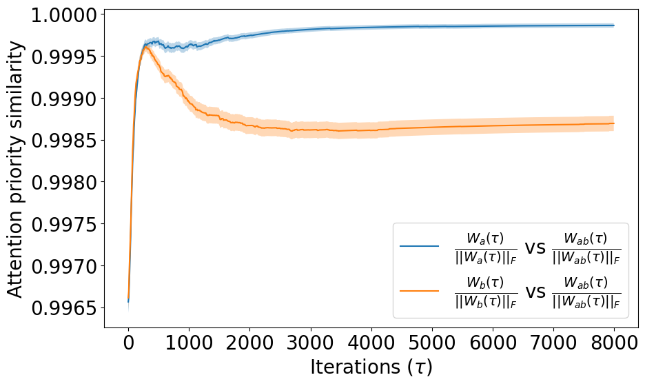
Figure 5: Convergence of attention priority similarity for $\frac{{\bf W}_{ab}(\tau)}{\|{\bf W}_{ab}(\tau)\|_{F}}$ relative to $\frac{{\bf W}_{a}(\tau)}{\|{\bf W}_{a}(\tau)\|_{F}}$ (blue) and $\frac{{\bf W}_{b}(\tau)}{\|{\bf W}_{a}(\tau)\|_{F}}$ (orange).

5 Explaining Topic Shifts

The formation of new SCCs when combining datasets suggests that the highest priority SCC for some input sequences may increase in size in this new setting. This also suggests that topic shifts may arise from ambiguity within an input sequence rather than a straightforward change in topic. In our analogy on the oracle, gaining knowledge of both Topic A and Topic B might cause a conversation to be naturally followed within Topic A or also outside Topic A. We introduce the following definition to characterize this phenomenon:

Definition 4 (ambiguous sequence).

Given DSET_a and DSET_b generated from two different topics $\mathbb{T}_{a}$ and $\mathbb{T}_{b}$. Denote $\mathbb{T}_{ab}$ as the combined topic defined by a combination of DSET_a and DSET_b. A sequence $\bf X$ that belongs to $\mathbb{T}_{a}$ is ambiguous in $\mathbb{T}_{ab}$ with respect to $\mathbb{T}_{a}$ if $\tilde{\bf W}_{ab}$ does not keep topic $\mathbb{T}_{a}$ for ${\bf X}$, but $\widehat{\mathcal{G}}_{a}^{(\bar{x})}({\bf X})\subset\widehat{\mathcal{G}}_{ab}^{(\bar{x})}({\bf X})$.

Definition 4 defines an ambiguous sequence as one where the highest-probability next-token predictions include tokens from both within and outside the input topic, reflecting natural ambiguity from overlapping topics. For instance, the input sequence ${\bf X}=[{\bf e}_{1},{\bf e}_{4},{\bf e}_{1},{\bf e}_{4}]^{\top}$ in Figure 4 (middle) belongs to both $\mathbb{T}_{a}$ and $\mathbb{T}_{b}$. $\widehat{\mathcal{G}}_{a}^{(4)}({\bf X})$ is $\{{\bf e}_{1}\}$, as depicted in $\mathcal{G}_{a}^{(4)}$ from Figure 3 (left) and $\widehat{\mathcal{G}}_{ab}^{(4)}({\bf X})$ is $\{{\bf e}_{1},{\bf e}_{4}\}$, as shown in $\mathcal{G}_{ab}^{(4)}$ from Figure 3 (right). $\widehat{\mathcal{G}}_{a}^{(4)}({\bf X})$ is the subset of $\widehat{\mathcal{G}}_{ab}^{(4)}({\bf X})$, though $\hat{y}_{{\bf w}_{ab}}\not\in\widehat{\mathcal{G}}_{a}^{(4)}({\bf X})$. We can argue that the next token predicted from an ambiguous sequence cannot be considered as a topic change, as it lacks the clear trigger phenomenon observed in human cognition. To address this, we propose a formal definition for a topic change:

Definition 5 (change of topic).

Given DSET_a and DSET_b generated from two topics $\mathbb{T}_{a}$ and $\mathbb{T}_{b}$, and a sequence $\bf X$ that belongs to $\mathbb{T}_{a}$. The weight matrix $\tilde{\bf W}_{ab}$ changes topic $\mathbb{T}_{a}$ for sequence ${\bf X}$ if $\tilde{\bf W}_{ab}$ does not keep topic $\mathbb{T}_{a}$ for ${\bf X}$ and $\bf X$ is not ambiguous in $\mathbb{T}_{ab}$ with respect to $\mathbb{T}_{a}$.

In Figure 4, ${\bf W}_{ab}$ for the last input sequence ${\bf X}=[{\bf e}_{5},{\bf e}_{4},{\bf e}_{4},{\bf e}_{4}]^{\top}$ can be considered as change of topic.

Building on the formal definitions of topic continuity, ambiguous sequences, and topic changes, we now present a necessary condition for a sequence to induce a topic change. This is achieved by introducing our final definition, grounded in the highest-priority SCC as determined by the order in the attention layer. Now, our second key result.

Definition 6 (highest priority SCC).

Consider a sequence ${\bf X}$ that belongs to $\mathbb{T}$. We define $\dot{\mathcal{G}}^{(\bar{x})}({\bf X})\subseteq\mathcal{G}^{(\bar{x})}$ as the highest priority SCC for ${\bf X}$ in $\mathcal{G}^{(\bar{x})}$ such that $\forall{x}_{i}\in\dot{\mathcal{G}}^{(\bar{x})}({\bf X})$ and ${x}_{j}\in\mathcal{G}^{(\bar{x})}$ we have $(x_{i}\Rightarrow x_{j})\in\mathcal{G}^{(\bar{x})}$ or $(x_{i}\asymp x_{j})\in\mathcal{G}^{(\bar{x})}$.

Theorem 4.

Under the same settings and assumptions on datasets and training in Theorem 3, let ${\bf X}$ be a sequence that belongs to $\mathbb{T}_{a}$. If $\tilde{\bf W}_{ab}$ changes topic $\mathbb{T}_{a}$ for $\bf X$ then $\exists x_{j}\not\in\dot{\mathcal{G}}_{a}^{(\bar{x})}(\bf X)$ such that $\forall x_{i}\in\dot{\mathcal{G}}_{a}^{(\bar{x})}(\bf X)$, the number of times ${\bf x}_{j}$ appears in $\bf X$ is greater than the number of times ${\bf x}_{i}$ appears in $\bf X$.

Theorem 4 implies that, for a given sequence X from $\mathbb{T}_{a}$ and its corresponding TPG, a necessary condition for a topic change is the presence of a lower-priority token that appears more frequently than any of the higher-priority tokens. This can be intuitively understood through our analogy: if the oracle is following a conversation on Topic A but the conversation contains repeated components with lower importance in Topic A, its knowledge of Topic B may steer the response toward Topic B, thereby initiating a shift away from Topic A. A natural question arises: what do these findings imply in practice? Specifically, how does the probability of change of topic behaves as the input sequence length increases or as the ambiguity between topics grows? The following theorem provides insights into these dynamics.

Theorem 5.

Under same settings and assumptions on datasets and training in Theorem 3, let $\bf X$ be a sequence that belongs to $\mathbb{T}_{a}$ with no repeated tokens, and $l$ be the number of elements in $\dot{\mathcal{G}}_{a}^{(\bar{x})}({\bf X})$. Let ${\bf X}^{\prime}=[{\bf x}_{1}^{\prime}\ {\bf x}_{2}^{\prime}\ \cdots\ {\bf x}_{T}^{\prime}]^{\top}$ be a random sequence of iid random tokens sampled from $\bf X$ such that for a fixed $p$, $p=\min_{x\in\dot{\mathcal{G}}_{a}^{(\bar{x})}({\bf X})}\mathbb{P}\left({\bf x}_{i}^{\prime}={\bf x}\right)$. We have:

1. If $p>\max_{x\not\in\dot{\mathcal{G}}_{a}^{(\bar{x})}({\bf X})}\mathbb{P}\left({\bf x}_{i}^{\prime}={\bf x}\right)$ then

   $\mathbb{P}(\tilde{\bf W}_{ab}$ changes topic $\mathbb{T}_{a}$ for sequence ${\bf X}^{\prime})\to 0$ as $T\to\infty.$

2. If $l$ increases then the probability that $\exists x_{j}^{\prime}\not\in\dot{\mathcal{G}}_{a}^{(\bar{x})}(\bf X)$ such that $\forall x_{i}^{\prime}\in\dot{\mathcal{G}}_{a}^{(\bar{x})}(\bf X)$, the number of times ${\bf x}_{j}^{\prime}$ appears in $\bf X^{\prime}$ is greater than the number of times ${\bf x}_{i}^{\prime}$ appears in $\bf X^{\prime}$ does not increase.

There are two implications of this theorem. First, as the input sequence length increases sufficiently, the likelihood of topic changes vanishes. Second, notice that increasing $l$ increases the probability of overlap between topics, and it also decreases the probability of satisfying the necessary conditions for a topic change, effectively creating a bound on the frequency of topic changes. In practice, consider the oracle analogy: if the oracle is following a sufficiently long conversation on a specific topic, it becomes exceedingly unlikely to shift topics. Similarly, as topics A and B become more interconnected, this increased ambiguity does not lead to more topic changes; rather, it may reduce their occurrence. This contrasts with human cognition, where longer conversations and greater inter-connectivity of knowledge increase the likelihood of spontaneous shifts.

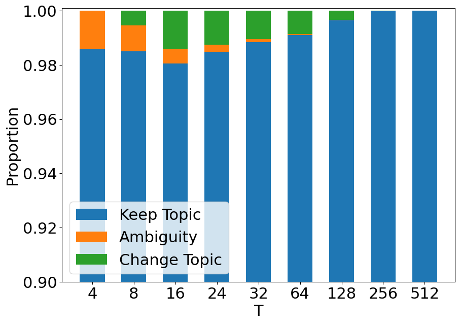
(a) Length of sequences.

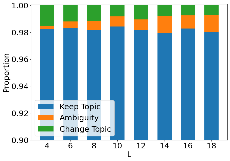
(b) Overlap between topics.

Figure 6: The proportion of keep topic (topic continuity), ambiguity (ambiguous sequence), and change topic (change of topic) as (a) the input sequence length increases and (b) the overlap between topics increases.

To illustrate Theorem 5, we conduct simulations following the same implementation settings as described in Section 4. We approximate $\tilde{\mathbf{W}}_{a}$ and $\tilde{\mathbf{W}}_{ab}$ as the results obtained after $\tau=8000$ iterations of Algo-GD. We quantify the proportion of test sequences in which $\tilde{{\bf W}}_{ab}$ keeps $\mathbb{T}_{a}$ (keep topic), proportion of ambiguous sequences in $\mathbb{T}_{ab}$ (ambiguity) and proportion of times in which $\tilde{{\bf W}}_{ab}$ changes topic (change topic). First, we explore the effect of longer sequences by varying the length $T$ of the test sequences $\bf Z$. We increase $T$ from 4 to 512. Figure 6(a) illustrates how the proportion of change topic decreases as $T$ increases. Second, we investigate the effect of overlapping topics by generating TPGs with an increased number of edges $L$. Intuitively, a higher $L$ results in an increase $l$ and a greater overlap between TPGs of different topics. We vary $L$ from 4 to 18. Figure 6(b) demonstrates that as $L$ increases, ambiguity increases, while proportion of change topic decreases. These two findings contrast with expectations derived from human cognition but align with the result of Theorem 5. Lastly, among the 85000 test sequences generated for these experiments, 99.98% satisfy Theorem 4 (i.e., topic changes occur when a low-priority token appears more frequently than high-priority tokens). The remaining 0.02% mismatched cases were solely due to minor approximation discrepancies in the attention softmax. These results validate Theorem 4 (simulation details in Appendix C).

Related Work

Training and generalization of Transformer. (1) Properties of Self-attention and Softmax. The self-attention mechanism employs the softmax function to selectively emphasize different parts of the input. Gu et al., (2024), Goodfellow et al., (2016), and Deng et al., (2023) underscore the pivotal role of the softmax function in shaping attention distributions, influencing how models process and prioritize information within input sequences. Bombari and Mondelli, (2024) examined the word sensitivity of attention layers, revealing that softmax-based attention-layers are adept at capturing the significance of individual words. Despite these strengths, recent researches have highlighted limitations of the softmax function (Saratchandran et al.,, 2024; Deng et al.,, 2023). (2) Optimization in attention-based models. Additionally, recent researches interpret Transformer models as kernel machines, akin to support vector machines (SVMs), with self-attention layers performing maximum margin separation in the token space (Tarzanagh et al., 2023a, ; Tarzanagh et al., 2023b, ; Li et al., 2024b, ; Julistiono et al.,, 2024). (3) Chain-of-Thought and In-Context Learning. Moreover, transformers exhibit remarkable abilities in generalization through in-context learning (ICL), where models effectively learn from contextual cues during inference (Brown et al.,, 2020; Xie et al.,, 2022; Olsson et al.,, 2022). Chain-of-Thought (CoT) prompting (Wei et al.,, 2022; Zhou et al.,, 2023; Shao et al.,, 2023; Li et al., 2024a, ) enhances this by breaking down reasoning processes into intermediate steps, highlighting the emergent reasoning abilities of transformers. (4) Improvement efficiency of transformers. Recent advancements aim to improve the computational efficiency of transformers (Kitaev et al.,, 2020; Choromanski et al.,, 2021; Sukhbaatar et al.,, 2019; Wang et al.,, 2020), ensuring their viability for large-scale deployment while maintaining or enhancing their representational capabilities.

Next token prediction in LLMs. (1) Theoretical and architectural innovations. Shannon, (1951)’s foundational work laid the groundwork for estimating the predictability of natural language sequences, providing a basis for subsequent advances in language modeling. Recent studies have expanded our understanding of how LLMs anticipate future tokens from internal hidden states, offering valuable insights into the efficiency and effectiveness of transformer-based architectures (He and Su,, 2024; Pal et al.,, 2023; Shlegeris et al.,, 2024). Despite their impressive predictive capabilities, these models face fundamental limitations. For instance, Bachmann and Nagarajan, (2024) highlights the shortcomings of teacher-forced training, emphasizing how this approach can fail and suggesting strategies to improve model robustness. (2) Efficiency and Optimization. Goyal et al., (2024) introduces a novel method that incorporates a deliberate computation step before output generation, enhancing reasoning capabilities. Additionally, Gloeckle et al., (2024) advocates for multi-token prediction, which significantly improves both efficiency and speed.

Self-Attention and topic dynamics. Advancements in the field has significantly advanced our understanding of how self-attention mechanisms in transformers manage evolving semantic contexts, with works have explored various aspects of topic modeling, including dynamic topic structures (Miyamoto et al.,, 2023), hierarchical relationships (Lin et al.,, 2024), topic-aware attention (Panwar et al.,, 2021), and mechanistic analysis of topic structure (Li et al.,, 2023). While these works provide insights into managing static and hierarchical topic structures, our work focuses on the topic changes during next-token prediction within the given input sequences from a specific topic.

6 Discussion

Our exploration with a simple single-layer attention model reveals fundamental clues on the distinctions between human and AI conversational dynamics. While humans naturally shift topics through curiosity or contextual triggers, the model remains anchored to the context. These observations suggest that human-like spontaneity in topic changes demands mechanisms beyond pattern recognition, raising deeper questions about the nature of interaction and highlighting the importance of creativity in advancing conversational AI.

However, our analysis relies on the simplified single-layer self-attention setting from Li et al., 2024b . This does not directly extend to complex modern LLMs with deeper architectures and varied training goals. Future work will explore how these findings translate to more intricate models, examining their ability to change topics. Moreover, the recurring theme of topic continuity characterized in this work opens new avenues for applications, such as automatic change topic detection in conversational AI based on discrepancies between model predictions and speaker outputs.

Appendix A Technical Proofs

A.1 Proofs of Lemmas

A.1.1 Proof of Lemma 2

Let ${\bf a}=\mathbb{S}({\bf X}\tilde{\bf W}\bar{{\bf x}})$.

$${\bf C}f_{\tilde{\bf W}}({\bf X}) ={\bf C}\left({\bf X}^{\top}\mathbb{S}\left({\bf X}\tilde{\bf W}\bar{{\bf x}}\right)\right)$$ (3)

$$={\bf C}\left({\bf X}^{\top}{\bf a}\right)$$ (4)

$$=\begin{bmatrix}\sum_{i=1}^{T}a_{i}\,({\bf c}_{1}^{\top}\cdot{\bf x}_{i})\\ \sum_{i=1}^{T}a_{i}\,({\bf c}_{2}^{\top}\cdot{\bf x}_{i})\\ \vdots\\ \sum_{i=1}^{T}a_{i}\,({\bf c}_{K}^{\top}\cdot{\bf x}_{i})\end{bmatrix}.$$ (5)

Let $k_{i}$ be the number of times token ${\bf x}_{i}$ appears in ${\bf X}$. Then,

$$\left[{\bf C}f_{\tilde{\bf W}}({\bf X})\right]_{x_{i}}=k_{i}a_{i}.$$

From Assumption 3 we have that

$$\left[{\bf C}f_{\tilde{\bf W}}({\bf X})\right]_{x_{i}}=\left[{\bf C}f_{\tilde{\bf W}}({\bf X})\right]_{x_{j}} \iff a_{i}=a_{j}$$ (7)

$$\iff(x_{i}\asymp x_{j})\in\mathcal{G}^{(\bar{x})}\text{ or }x_{i}=x_{j}.$$ (8)

If $x_{i}\neq x_{j}$ then $x_{i}$ and $x_{j}$ are in the same SCC.∎

A.1.2 Proof of Lemma 6

Lemma 6.

For an input sequence ${\bf X}$ that belongs to $\mathbb{T}$ and $i,j\in[T]$,

• $[\mathbb{S}({\bf X}\tilde{\bf W}\bar{{\bf x}})]_{i}=[\mathbb{S}({\bf X}\tilde{\bf W}\bar{{\bf x}})]_{j}\iff(x_{i}\asymp x_{j})\in\mathcal{G}^{(\bar{x})}$ or $i=j$.

• $[\mathbb{S}({\bf X}\tilde{\bf W}\bar{{\bf x}})]_{i}<[\mathbb{S}({\bf X}\tilde{\bf W}\bar{{\bf x}})]_{j}\iff(x_{j}\Rightarrow x_{i})\in\mathcal{G}^{(\bar{x})}$.

• $[\mathbb{S}({\bf X}\tilde{\bf W}\bar{{\bf x}})]_{i}>[\mathbb{S}({\bf X}\tilde{\bf W}\bar{{\bf x}})]_{j}\iff(x_{i}\Rightarrow x_{j})\in\mathcal{G}^{(\bar{x})}$.

Proof.

Since $\bf X$ belongs to $\mathbb{T}$, $\forall{\bf x}\in{\bf X}$ we have $x\in\mathcal{G}^{(\bar{x})}$, therefore from the construction of TPGs by Li et al., 2024b , for every ${\bf x}_{i},{\bf x}_{j}\in{\bf X}$ we have one of the these relationships: $(x_{i}\Rightarrow x_{j})$, $(x_{j}\Rightarrow x_{i})$, $(x_{i}\asymp x_{j})$ or $x_{i}=x_{j}$. From the constraints in Algo-GD:

• $[\mathbb{S}({\bf X}\tilde{\bf W}\bar{{\bf x}})]_{i}=[\mathbb{S}({\bf X}\tilde{\bf W}\bar{{\bf x}})]_{j}\iff({\bf x}_{i}-{\bf x}_{j})^{\top}\tilde{\bf W}{\bar{x}}=0\iff(x_{j}\asymp x_{i})\in\mathcal{G}^{(\bar{x})}\text{ or }i=j$.

• $[\mathbb{S}({\bf X}\tilde{\bf W}\bar{{\bf x}})]_{i}>[\mathbb{S}({\bf X}\tilde{\bf W}\bar{{\bf x}})]_{j}\iff({\bf x}_{i}-{\bf x}_{j})^{\top}\tilde{\bf W}{\bar{x}}>1\iff(x_{j}\Rightarrow x_{i})\in\mathcal{G}^{(\bar{x})}$.

• $[\mathbb{S}({\bf X}\tilde{\bf W}\bar{{\bf x}})]_{i}<[\mathbb{S}({\bf X}\tilde{\bf W}\bar{{\bf x}})]_{j}\iff({\bf x}_{i}-{\bf x}_{j})^{\top}\tilde{\bf W}{\bar{x}}<1\iff(x_{i}\Rightarrow x_{j})\in\mathcal{G}^{(\bar{x})}$.

∎

A.1.3 Proof of Lemma 7

Lemma 7.

For an input sequence ${\bf X}$ that belongs to $\mathbb{T}$,

$$\dot{\mathcal{G}}^{(\bar{x})}({\bf X})=\left\{x_{i}\ |\ [\mathbb{S}({\bf X}\tilde{\bf W}\bar{{\bf x}})]_{i}=\|\mathbb{S}({\bf X}\tilde{\bf W}\bar{{\bf x}})\|_{\infty}\right\}.$$

Proof.

Let $G=\{x_{i}\ |\ [\mathbb{S}({\bf X}\tilde{\bf W}\bar{{\bf x}})]_{i}=\|\mathbb{S}({\bf X}\tilde{\bf W}\bar{{\bf x}})\|_{\infty}\}$. From Lemma 6 $\forall x_{i},x_{j}\in G$, $(x_{i}\asymp x_{j})\in\mathcal{G}^{(\bar{x})}$. Therefore all elements in $G$ belong to the same SCC. Also from Lemma 6, $\forall x_{i}\in G,x_{j}\not\in G$ we have $(x_{i}\Rightarrow x_{j})\in\mathcal{G}^{(\bar{x})}$. This means that every element in $G$ has the highest priority among tokens in $\bf X$ concluding our proof. ∎

A.2 Proof of Theorem 3

From construction, $\forall k\in[K]$, $\mathcal{G}_{a}^{(k)}\subseteq\mathcal{G}_{ab}^{(k)}$. This means that $\forall{\bf x}_{i},{\bf x}_{j}\in{\bf X}$, we have:

• if $(x_{i}\asymp x_{j})\in\mathcal{G}_{a}^{(\bar{x})}$ then $(x_{i}\asymp x_{j})\in\mathcal{G}_{ab}^{(\bar{x})}$

• if $(x_{j}\Rightarrow x_{i})\in\mathcal{G}_{a}^{(\bar{x})}$ then $(x_{j}\Rightarrow x_{i})\in\mathcal{G}_{ab}^{(\bar{x})}$ or $(x_{i}\asymp x_{j})\in\mathcal{G}_{ab}^{(\bar{x})}$

• if $(x_{i}\Rightarrow x_{j})\in\mathcal{G}_{a}^{(\bar{x})}$ then $(x_{i}\Rightarrow x_{j})\in\mathcal{G}_{ab}^{(\bar{x})}$ or $(x_{i}\asymp x_{j})\in\mathcal{G}_{ab}^{(\bar{x})}$

Combining with Lemma 6:

• $[\mathbb{S}({\bf X}\tilde{\bf W}_{a}\bar{{\bf x}})]_{i}=[\mathbb{S}({\bf X}\tilde{\bf W}_{a}\bar{{\bf x}})]_{j}\iff(x_{i}\asymp x_{j})\in\mathcal{G}_{a}^{(\bar{x})}$ or $i=j$, then $(x_{i}\asymp x_{j})\in\mathcal{G}_{ab}^{(\bar{x})}$ or $i=j\iff[\mathbb{S}({\bf X}\tilde{\bf W}_{ab}\bar{{\bf x}})]_{i}=[\mathbb{S}({\bf X}\tilde{\bf W}_{ab}\bar{{\bf x}})]_{j}$

• $[\mathbb{S}({\bf X}\tilde{\bf W}_{a}\bar{{\bf x}})]_{i}<[\mathbb{S}({\bf X}\tilde{\bf W}_{a}\bar{{\bf x}})]_{j}\iff(x_{j}\Rightarrow x_{i})\in\mathcal{G}_{a}^{(\bar{x})}$ then $(x_{j}\Rightarrow x_{i})\in\mathcal{G}_{ab}^{(\bar{x})}$ or $(x_{i}\asymp x_{j})\in\mathcal{G}_{ab}^{(\bar{x})}\iff[\mathbb{S}({\bf X}\tilde{\bf W}_{ab}\bar{{\bf x}})]_{i}\leq[\mathbb{S}({\bf X}\tilde{\bf W}_{ab}\bar{{\bf x}})]_{j}$

• $[\mathbb{S}({\bf X}\tilde{\bf W}_{a}\bar{{\bf x}})]_{i}>[\mathbb{S}({\bf X}\tilde{\bf W}_{a}\bar{{\bf x}})]_{j}\iff(x_{i}\Rightarrow x_{j})\in\mathcal{G}_{a}^{(\bar{x})}$ then $(x_{i}\Rightarrow x_{j})\in\mathcal{G}_{ab}^{(\bar{x})}$ or $(x_{i}\asymp x_{j})\in\mathcal{G}_{ab}^{(\bar{x})}\iff[\mathbb{S}({\bf X}\tilde{\bf W}_{ab}\bar{{\bf x}})]_{i}\geq[\mathbb{S}({\bf X}\tilde{\bf W}_{ab}\bar{{\bf x}})]_{j}$∎

A.3 Proof of Theorem 4

Let ${\bf a}=\mathbb{S}({\bf X}\tilde{\bf W}_{a}\bar{{\bf x}})$ and ${\bf b}=\mathbb{S}({\bf X}\tilde{\bf W}_{ab}\bar{{\bf x}})$. Without loss of generality, suppose ${\bf a}$ is in decreasing order $a_{1}\geq\cdots\geq a_{T}$. From Theorem 3, we also have $b_{1}\geq\cdots\geq b_{T}$. Let $k_{i}$ be the number of times token ${\bf x}_{i}$ appears in ${\bf X}$. Following an analogous procedure as in Lemma 2 we get

$$\left[{\bf C}f_{\tilde{\bf W}_{a}(\tau)}({\bf X})\right]_{x_{i}}=k_{i}a_{i}$$ (9)

$$\left[{\bf C}f_{\tilde{\bf W}_{ab}(\tau)}({\bf X})\right]_{x_{i}}=k_{i}b_{i}$$ (10)

We will proof the contrapositive: If $\exists x_{i}\in\dot{\mathcal{G}}_{a}^{(\bar{x})}({\bf X})$ such that $k_{i}\geq k_{j}$ for all $j\in[K]$, then there is no change of topic, so $\tilde{\bf W}_{ab}$ keeps topic $\mathbb{T}_{a}$ for input sequence $\bf X$, or $\bf X$ is ambiguous in $\mathbb{T}_{ab}$ with respect to $\mathbb{T}_{a}$.

From Lemma 7, if $x_{i}\in\dot{\mathcal{G}}_{a}^{(\bar{x})}({\bf X})$, we have $a_{i}\geq a_{j}$ for all $j\in[K]$. Suppose $\exists x_{i}\in\dot{\mathcal{G}}_{a}^{(\bar{x})}({\bf X})$ such that $k_{i}\geq k_{j}$ for all $j\in[K]$, we have that $k_{i}a_{i}\geq k_{j}a_{j}$ for all $j\in[K]$ then $x_{i}\in\widehat{\mathcal{G}}_{a}^{(\bar{x})}({\bf X})$. Analogously since $b_{i}\geq b_{j}$, $x_{i}\in\widehat{\mathcal{G}}_{ab}^{(\bar{x})}({\bf X})$. If $\exists x_{l}\in\widehat{\mathcal{G}}_{a}^{(\bar{x})}({\bf X})$ with $x_{l}\neq x_{i}$ then $k_{l}a_{l}\geq k_{j}a_{j}$ for all $j\in[K]$, then $k_{l}a_{l}=k_{i}a_{i}$. Therefore from Assumption 3 and Lemma 7, $(x_{l}\asymp x_{i})\in\mathcal{G}_{a}^{(\bar{x})}$. Analogously $(x_{l}\asymp x_{i})\in\mathcal{G}_{ab}^{(\bar{x})}$. This means that if $\exists x_{i}\in\dot{\mathcal{G}}_{a}^{(\bar{x})}({\bf X})$ such that $k_{i}\geq k_{j}$ for all $j\in[K]$, then $\widehat{\mathcal{G}}_{a}^{(\bar{x})}({\bf X})\subseteq\widehat{\mathcal{G}}_{ab}^{(\bar{x})}({\bf X})$. Then $\tilde{\bf W}_{ab}$ keeps topic $\mathbb{T}_{a}$ for input sequence $\bf X$, or $\bf X$ is ambiguous in $\mathbb{T}_{ab}$ with respect to $\mathbb{T}_{a}$.∎

A.4 Proof of Theorem 5

1. This is a direct consequence from the law of large numbers. If $T\to\infty$ the proportion of each token will match the probability. Since $p>\max_{{\bf x}\not\in\dot{\mathcal{G}}_{a}^{(\bar{x})}({\bf X})}\mathbb{P}\left({\bf x}_{i}^{\prime}={\bf x}\right)$, then the probability that $\exists x_{j}^{\prime}\not\in\dot{\mathcal{G}}_{a}^{(\bar{x})}(\bf X)$ such that $\forall x_{i}^{\prime}\in\dot{\mathcal{G}}_{a}^{(\bar{x})}(\bf X)$, the number of times ${\bf x}_{j}^{\prime}$ appears in $\bf X^{\prime}$ is greater than the number of times ${\bf x}_{i}^{\prime}$ appears in $\bf X^{\prime}$ will go to zero, and therefore the probability of change topics will do it also.

2. Without loss of generality suppose $\dot{\mathcal{G}}_{a}^{(\bar{x})}({\bf X})=\{x_{1},x_{2},\cdots,x_{l}\}$. Clearly if we prove the result assuming $\forall x\in\dot{\mathcal{G}}_{a}^{(\bar{x})}({\bf X}),\ p=\mathbb{P}\left({\bf x}_{i}^{\prime}={\bf x}\right)$, we will also have it for the more general case $p=\min_{{\bf x}\in\dot{\mathcal{G}}_{a}^{(\bar{x})}({\bf X})}\mathbb{P}\left({\bf x}_{i}^{\prime}={\bf x}\right)$.

   Let ${\bf X}_{l}^{\prime}=[{\bf x}_{1,l}^{\prime}\ {\bf x}_{2,l}^{\prime}\ \cdots\ {\bf x}_{T,l}^{\prime}]^{\top}$ be a random sequences generated as described in the theorem, where the size of $\dot{\mathcal{G}}_{a}^{(\bar{x})}({\bf X})$ is $l$. Let $k_{i,l}$ be the number of times ${\bf x}_{i}$ is selected in ${\bf X}_{l}^{\prime}$ . Let $A_{l}=\max_{1\leq i\leq l}k_{i,l}$ and $B_{l}=\max_{l+1\leq i\leq K}k_{i,l}$. Let $P(l)=\mathbb{P}(B_{l}>A_{l})$. We want to prove $P(l+1)\leq P(l)$. We construct a coupling between ${\bf X}_{l}^{\prime}$ and ${\bf X}_{l+1}^{\prime}$ by performing $T$ independent trials. For each trial $i$ we generate a uniform random variable $U_{i}$ in $[0,1]$ and we choose tokens in ${\bf X}_{l}^{\prime}$ and ${\bf X}_{l+1}^{\prime}$ in this way:

   • If $U_{i}\leq pl$ both the selected tokens $x_{i,l}^{\prime}$ and $x_{i,l+1}^{\prime}$ are in $\{x_{1},x_{2},\cdots,x_{l}\}$.

   • If $pl<U_{i}\leq p(l+1)$, we select $x_{i,l}^{\prime}=x_{l+1}$ if $U_{i}\leq pl+q$ or $x_{i,l}^{\prime}=x_{l+2}$ otherwise, and we select $x_{i,l+1}^{\prime}=x_{l+1}$; where $q$ is the probability of choosing $x_{l+1}$ in ${\bf X}_{l}^{\prime}$. Since $p>q$, there is an interval where $x_{i,l}=x_{l+2}$ but $x_{i,l+1}=x_{l+1}$.

   • If $U_{i}>p(l+1)$, then both the selected tokens $x_{i,l}^{\prime}$ and $x_{i,l+1}^{\prime}$ are in $\{x_{l+2},x_{2},\cdots,x_{l}\}$. Notice that the probability of choosing $x_{i}$ in ${\bf X}_{l+1}^{\prime}$ for $i\geq l+2$ decreases because $p$ is constant.

   From the previous coupling we have that $k_{i,l}=k_{i,l+1}$ for $1\leq i\leq l$, $k_{l+1,l}\leq k_{l+1,l+1}$ for $i=l+1$, and $k_{i,l}\geq k_{i,l+1}$ for $i\geq l+2$. This means that $A_{l+1}=\max(A_{l},k_{l+1,l+1})\geq A_{l}$ and $B_{l+1}=\max_{l+2\leq i\leq K}k_{i,l+1}\leq B_{l}$. Therefore $P(l+1)=\mathbb{P}(B_{l+1}>A_{l+1})\leq\mathbb{P}(B_{l}>A_{l})=P(l)$.

∎

Appendix B Detailed Explanation of Assumption 4

As illustrated in Figure 7, the dataset for $\mathbb{T}_{a}$ and the dataset for $\mathbb{T}_{b}$ demonstrate interchangeability with $\mathcal{G}_{a}^{(4)}$ and $\mathcal{G}_{b}^{(4)}$, respectively.

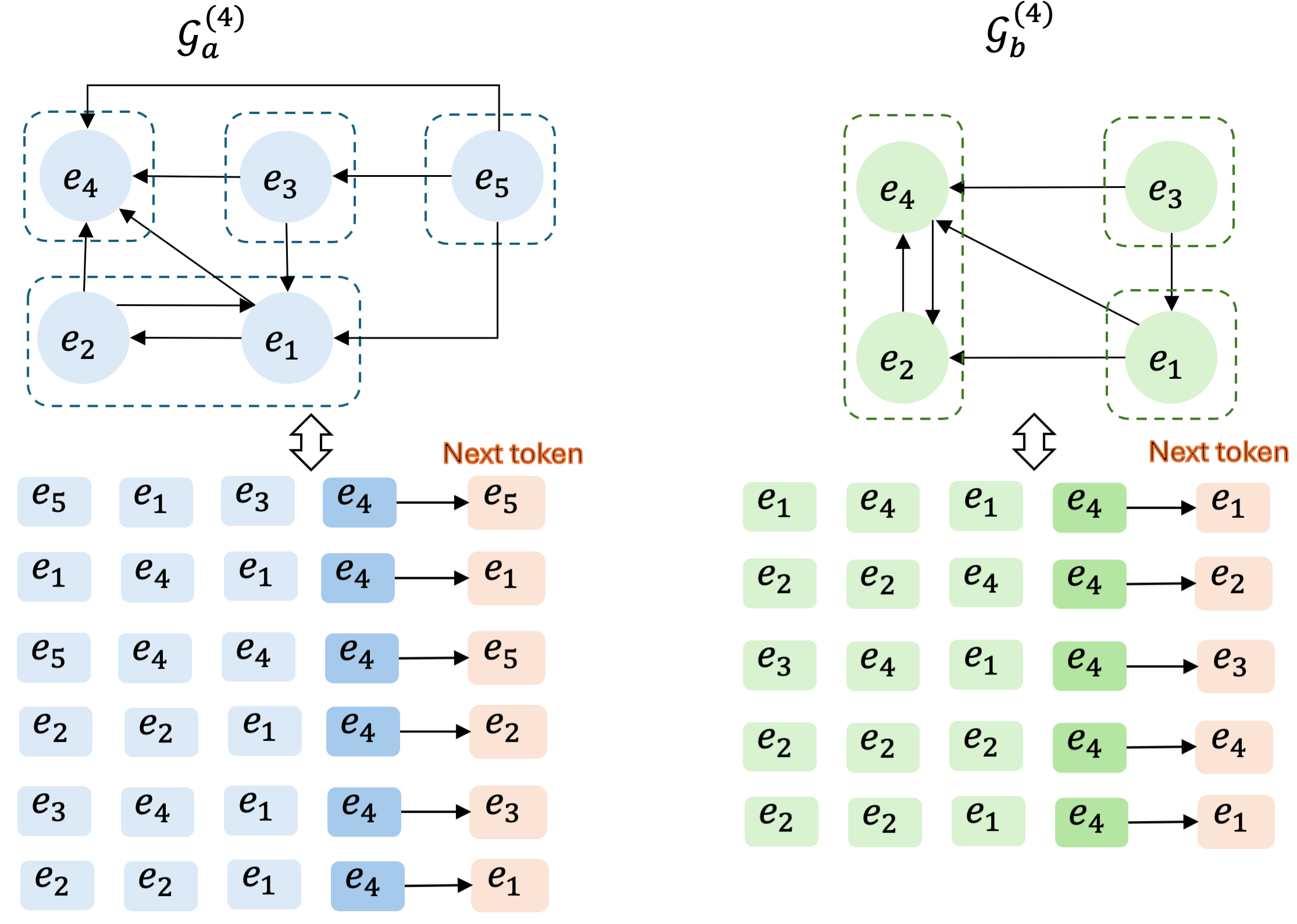
Figure 7: Illustration of Assumption 4. Here are two datasets related to the TPGs, $\mathcal{G}_{a}^{(4)}$ and $\mathcal{G}_{b}^{(4)}$, from Figure 3. From the directed arrows in $\mathcal{G}_{a}^{(4)}$, we can generate a dataset with the last token $\bf{e}_{4}$ for $\mathbb{T}_{a}$, which can reconstruct back the $\mathcal{G}_{a}^{(4)}$. A similar process applies for the $\mathcal{G}_{b}^{(4)}$.

Appendix C Detailed Simulation Studies

C.1 Simulation Process

Theoretical TPGs generation. For each token $e_{k}$, $L$ edges are randomly selected to construct the theoretical TPG $\mathcal{G}^{(k)}_{theor}$ for $e_{k}$ , ensuring that $e_{k}$ is involved, as either a source or destination node. Based on these selected edges, we add additional edges from $e_{k}$ to all other tokens included in $L$ edges, thereby ensuring that all tokens in $\mathcal{G}^{k}_{theor}$ can be reached by $e_{k}$. Thus, we obtain the theoretical TPGs $\{\mathcal{G}^{(k)}_{a,theor}\}^{K}_{k=1}$ for Topic A . This process is repeated to generate another group of theoretical TPGs $\{\mathcal{G}^{(k)}_{b,theor}\}^{K}_{k=1}$ for the Topic B. Let $\mathcal{G}^{(k)}_{a,theor}$ and $\mathcal{G}^{(k)}_{b,theor}$ combine for each $k$, we obtain the theoretical TPGs for topics combinations $\{\mathcal{G}^{(k)}_{ab,theor}\}^{K}_{k=1}$.

Training Dataset Generation. Generate training datasets DSET_a and DSET_b based on $\{\mathcal{G}^{(k)}_{a,theor}\}^{K}_{k=1}$ and $\{\mathcal{G}^{(k)}_{b,theor}\}^{K}_{k=1}$, respectively. For each input sequence in DSET, the sequence length $T_{train}$ is 4, which means ${\bf X}=[{\bf x}_{1}\ {\bf x}_{2}\ \cdots\ {\bf x}_{T_{train}}]^{\top}\in\mathbb{R}^{T_{train}\times d}$ with ${\bf x}_{i}$ from ${\bf E}=[{\bf e}_{1},{\bf e}_{2},...{\bf e}_{K}]^{\top}$. ${\bf e}_{k}$ is randomly selected as the last token and other tokens (other input tokens and the next predicted token) are chosen based on $\mathcal{G}^{(k)}_{theor}$. Specifically, the next token ${\bf e}_{T_{train}+1}$ is determined by sampling with the weighted probability in $\mathcal{G}^{(k)}_{theor}$, where the weight for each token corresponds to the number of outcoming edges. Given Assumption 2, we randomly choose the position of the next token in the input sequence. Then, the remaining input tokens are randomly selected from tokens connected by incoming edges from ${\bf e}_{k}$ (i.e., ${\bf e}_{k}\rightarrow{\bf e}_{i}$) and placed in the random position within the input sequence. This process is repeated $n$ times to generate training data for each topic respectively. Empirical TPGs $\{\mathcal{G}^{(k)}_{a,empir}\}^{K}_{k=1}$ and $\{\mathcal{G}^{(k)}_{b,empir}\}^{K}_{k=1}$ are derived from the training datasets DSET_a and DSET_b. According to Assumption 4, the empirical TPGs $\{\mathcal{G}^{(k)}_{empir}\}^{K}_{k=1}$ are expected to be identical to the theoretical TPGs $\{\mathcal{G}^{(k)}_{theor}\}^{K}_{k=1}$ for each topic. The experiments are conducted with $5000$ instances, with each parameter setting evaluated over 50 epochs, consisting of 100 sequences per epoch.

Trained attention weights. We employ a single-layer attention mechanism implemented in PyTorch. The model is trained using the SGD optimizer with a learning rate $\eta=0.01$ for $8000$ iterations. The training of attention weights is divided into two stages for each instance: (1) computing ${\bf W}^{\text{svm}}$ for each topic ; (2) get $\bf{W}(\tau)$ at each iteration for each topic. In Stage (1), prior to using the CVXPY package to get ${\bf W}^{\text{svm}}$, SCCs are identified for each TPG derived from the using Tarjan’s algorithm. Afterward, ${\bf W}^{\text{svm}}$ is normalized to ensure consistency in subsequence computations. In Stage (2), the $MLayerAttn$ function encapsulates the architecture of a single-layer attention-based model. The training function is then used to optimize the attention weights by minimizing the loss defined in ERM. Finally, the correlation between ${\bf W}^{\text{svm}}$ and $\bf{W}(\tau)$ is calculated using the dot product.

Next token prediction. To differentiate the input sequence length of the testing data from that of the training data, we introduce $T_{test}$. TPGs based on the training dataset DSET_a are utilized to generate test datasets consisting of 100 sequences from $\mathbb{T}_{a}$ per epoch. Specifically, the last token ${\bf x}_{T_{test}}$ of the test input sequence is randomly selected from $K$ tokens (i.e. ${\bf x}_{T_{test}}={\bf e}_{k}$) and the remaining input tokens are randomly chosen based on the SCCs of $\mathcal{G}^{k}_{a}$, where tokens with higher priority are assigned greater weights. For instance, in $\mathcal{G}^{4}_{a}$, tokens ${\bf e}_{1},{\bf e}_{2},{\bf e}_{4}$ are captured with the priority order ${\bf e}_{1}={\bf e}_{2}>{\bf e}_{4}$. The weights assigned to input tokens ${\bf e}_{1},{\bf e}_{2}$, and ${\bf e}_{4}$ are $0.4,0.4$, and $0.2$, respectively. It reflects that ${\bf e}_{1}$ and ${\bf e}_{2}$ are in the same higher-priority SCC, thus having greater weights compared to ${\bf e}_{4}$. Intuitively, tokens within the same SCC are more likely to co-occur than those from different SCCs. This approach enables the generated test input sequences to mimic real word relationships and reflect their contextual groupings. Following the generation of the test dataset from $\mathbb{T}_{a}$, the next tokens $\hat{y}_{\bf w_{a}}$ and $\hat{y}_{\bf w_{ab}}$ are predicted by Equation 1, with ${\bf W}_{a}$ and ${\bf W}_{ab}$ obtained from the last iteration. To reduce the potential numerical issues in the outputs, $\mathbb{S}({\bf X}{\bf W}\bar{{\bf x}})$ is rounded to three decimals, ensuring that tokens within the same SCC yield consistent softmax outputs. Our code for all simulations is available in ( ).

C.2 Experiments Results

In this section, we provide empirical evidence to support our findings outlined in Theorem 3, Theorem 4, and Theorem 5, offering detailed insights into the behavior of self-attention mechanisms for changing topics.

C.2.1 Simulation in Section 4

For Figure 5 we used $K=10,L=4,d=16,\text{and }T_{test}=T_{train}=4$, we also showed point-wise confidence intervals of rank similarities on all 5000 instances for each value of $\tau$.

C.2.2 Simulation in Section 5

Table 1: The proportion of keep topic, ambiguous, and change of topic with varying $T_{test}=\{4,8,16,24,32,64,128,256,512\}$.

$T_{test}$	Keep(%)	Ambiguous(%)	Change(%)
4	98.60 $\pm$ 1.54	1.40 $\pm$ 1.54	0.00 $\pm$ 0.00
8	98.50 $\pm$ 1.47	0.96 $\pm$ 1.11	0.54 $\pm$ 0.76
16	98.06 $\pm$ 1.33	0.54 $\pm$ 0.76	1.40 $\pm$ 1.07
24	98.48 $\pm$ 1.31	0.26 $\pm$ 0.44	1.26 $\pm$ 1.10
32	98.84 $\pm$ 1.15	0.12 $\pm$ 0.33	1.04 $\pm$ 1.03
64	99.10 $\pm$ 1.07	0.04 $\pm$ 0.20	0.86 $\pm$ 1.05
128	99.64 $\pm$ 0.53	0.02 $\pm$ 0.14	0.34 $\pm$ 0.52
256	99.98 $\pm$ 0.14	0.00 $\pm$ 0.00	0.02 $\pm$ 0.14
512	100.00 $\pm$ 0.00	0.00 $\pm$ 0.00	0.00 $\pm$ 0.00

Table 2: The proportion of keep topic, ambiguous, and change of topic with varying $L=\{4,6,8,10,12,14,16,18\}$.

L	Keep(%)	Ambiguous(%)	Change(%)
4	98.22 $\pm$ 1.43	0.26 $\pm$ 0.60	1.52 $\pm$ 1.31
6	98.30 $\pm$ 1.37	0.50 $\pm$ 0.68	1.20 $\pm$ 1.11
8	98.18 $\pm$ 1.49	0.68 $\pm$ 0.68	1.14 $\pm$ 1.23
10	98.42 $\pm$ 1.25	0.76 $\pm$ 0.85	0.82 $\pm$ 1.02
12	98.14 $\pm$ 1.32	0.82 $\pm$ 0.92	1.04 $\pm$ 0.97
14	97.96 $\pm$ 1.44	1.24 $\pm$ 1.06	0.80 $\pm$ 0.86
16	98.28 $\pm$ 1.33	0.98 $\pm$ 0.91	0.74 $\pm$ 0.85
18	98.02 $\pm$ 1.58	1.26 $\pm$ 1.14	0.72 $\pm$ 0.86

In Figure 6(a), we predict next tokens for 5000 test sequences from $\mathbb{T}_{a}$ with $T_{test}=\{4,8,16,24,32,64,128,256,512\}$, while fixing $L=4$, $d=16$, $T_{train}=4$, and $K=10$. The proportion of each scenario with varying $T$ is illustrated in Table 1. For Figure 6(b), we predict next tokens for 5000 test sequences (the sequence length is $T_{test}=20$) using models trained with $L=\{4,6,8,10,12,14,16,18\}$, $d=16$, $K=10$, and $T_{train}=4$. The proportion of each scenario with varying $L$ is illustrated in Table 2.

C.2.3 Additional experiments

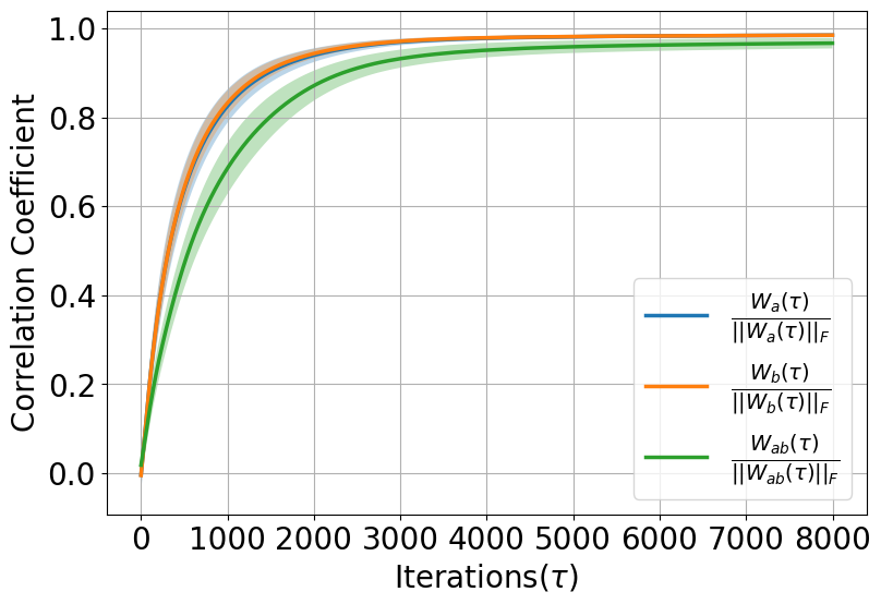
(a) $K=6,L=4$

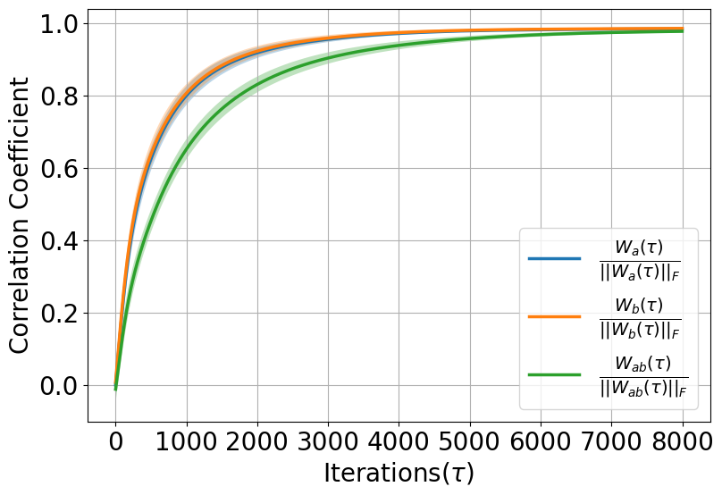
(b) $K=10,L=4$

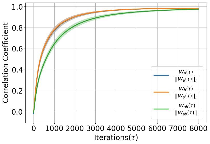
(c) $K=14,L=4$

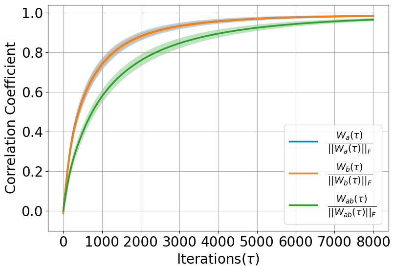
(d) $K=10,L=8$

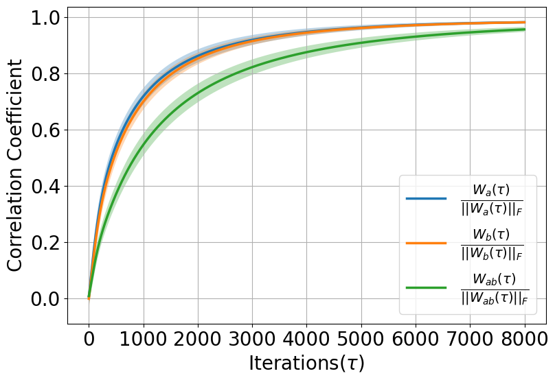
(e) $K=10,L=12$

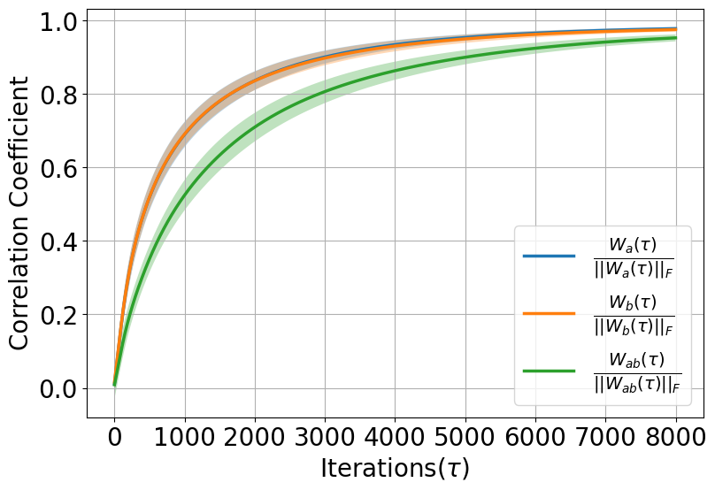
(f) $K=10,L=16$

Figure 8: Convergence of $\frac{{\bf W}_{a}(\tau)}{\|{\bf W}_{a}(\tau)\|_{F}}$(blue), $\frac{{\bf W}_{b}(\tau)}{\|{\bf W}_{b}(\tau)\|_{F}}$(orange), and $\frac{{\bf W}_{ab}(\tau)}{\|{\bf W}_{ab}(\tau)\|_{F}}$(green) for varying $K$ and $L$, with fixed $T_{train}=4$ and $d=16$.

Building upon the convergence experiments in Li et al., 2024b , our work demonstrates that the correlation coefficients $\langle{\bf W}_{ab}(\tau),{\bf W}^{\text{svm}}_{ab}\rangle/\langle\|{\bf W}_{ab}(\tau)\|_{F},\|{\bf W}^{\text{svm}}_{ab}\|_{F}\rangle$ (green lines) in Figure 8, measured with varying $K=\{6,10,14\}$ and $L=\{8,12,16\}$, approach to 1. These results indicate that Theorem 1 extends beyond individual topics to also capture the convergence dynamics of mixed-topics scenarios, albeit with relatively slower convergence. In these experiments, we fix $T_{train}=4$ and $d=16$. Each point represents the average over 5000 randomly generated instances, trained with 8000 iterations. The shaded area around each line represents the $95\%$ confidence interval, computed over 50 epochs.

C.3 Numerical Analysis of each Scenario in Figure 4

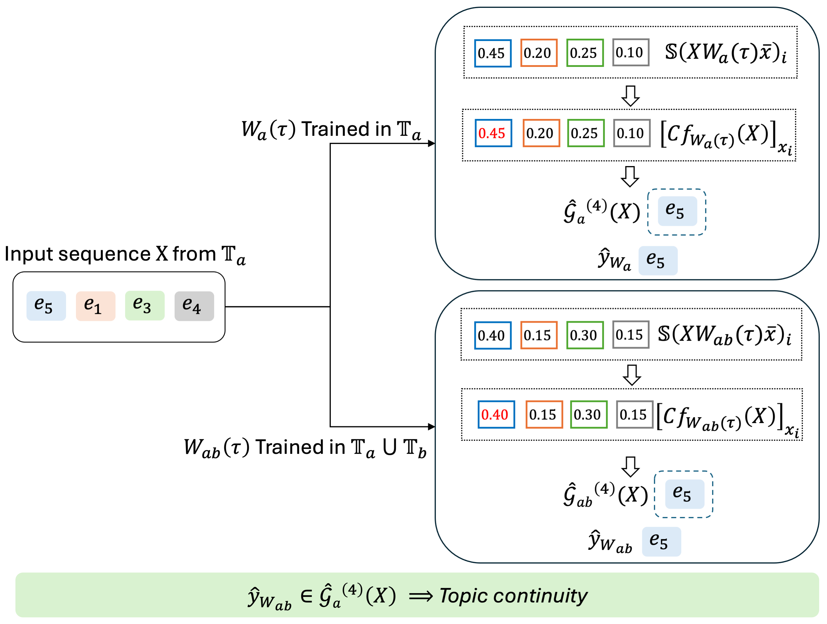
(a) Topic continuity.

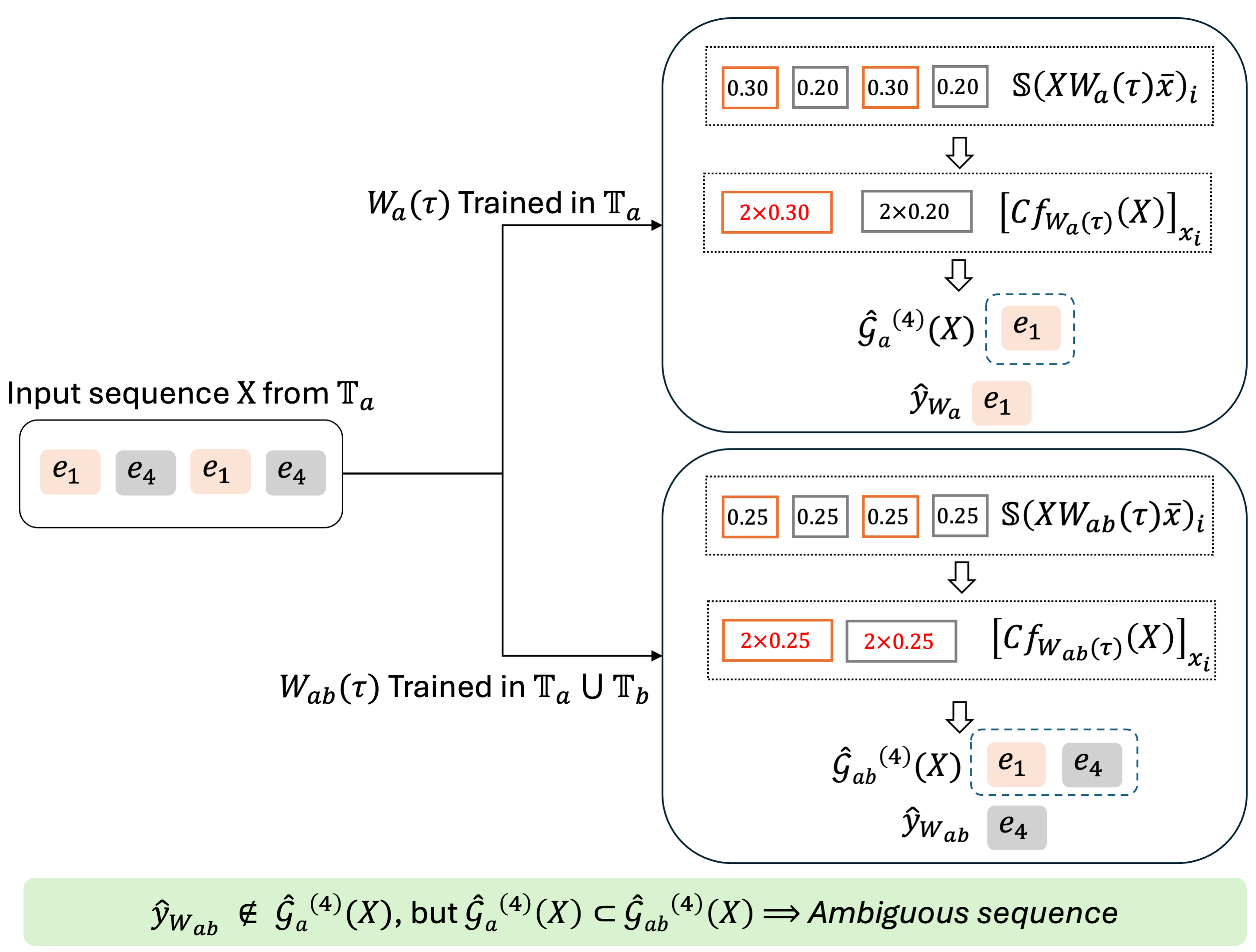
(b) Ambiguous sequence.

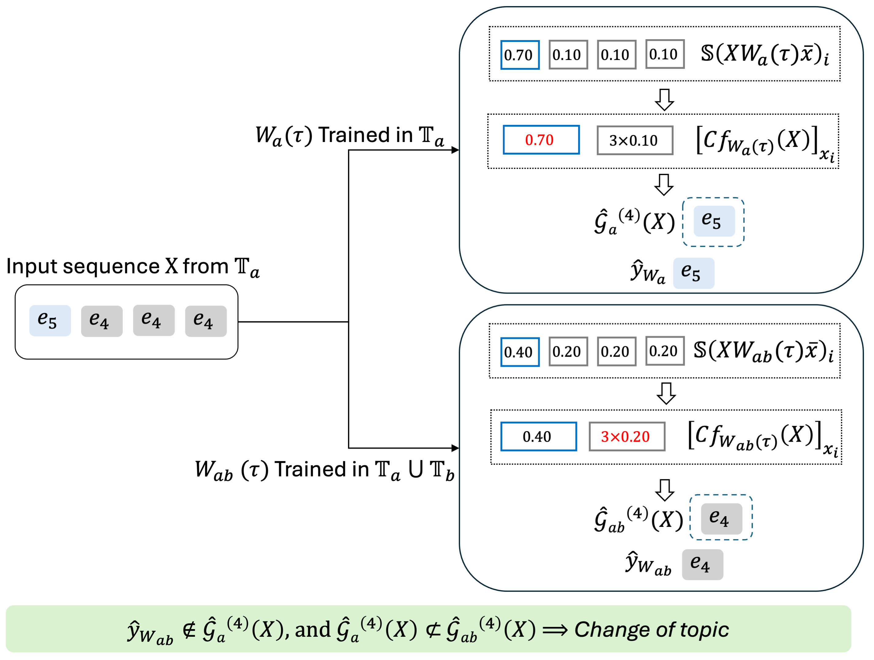
(c) Change of topic.

Figure 9: Numeric details for each scenario: (a) topic continuity, (b) ambiguous sequence, and (c) change of topic.

Figure 9 provides a numerical breakdown for each scenario in Figure 4. In Figure 9, each distinct color corresponds to a unique token within the input sequence $\bf X$, which consists of 4 tokens. ${\bf e}_{4}$ is the last token across all three input sequences. For each input sequence $\bf X$, we apply ${\bf W}_{a}(\tau)$ and ${\bf W}_{ab}(\tau)$ with $\tau=8000$ to predict the next token, yielding $\hat{y}_{{\bf W}_{a}}$ and $\hat{y}_{{\bf W}_{ab}}$, respectively.

Let $[\mathbb{S}({\bf X}{\bf W}_{a}(\tau){\bar{\bf x}})]_{i}=a_{i}$ and $[\mathbb{S}({\bf X}{\bf W}_{ab}(\tau){\bar{\bf x}})]_{i}=b_{i}$, for $i\in[T]$. Following Equation 9 and Equation 10, we compute $[Cf_{{\bf W}_{a}(\tau)}({\bf X})]_{x_{i}}$ and $[Cf_{{\bf W}_{ab}(\tau)}({\bf X})]_{x_{i}}$ to get the highest probability SCC and predict the next token for each input sequence.

Topic continuity. In Fig. 9(a), input sequence $\bf X$ consists of four unique tokens: ${\bf e}_{5}$, ${\bf e}_{1}$, ${\bf e}_{3}$, and ${\bf e}_{4}$. Based on $\mathcal{G}^{(4)}_{a}$ in Figure 3, the priority order of these tokens is ${\bf e}_{5}>{\bf e}_{3}>{\bf e}_{1}>{\bf e}_{4}$, with corresponding $a_{i}$ values: $0.45>0.25>0.20>0.1$. Since $[Cf_{{\bf W}_{a}(\tau)}({\bf X})]_{{\bf e}_{5}}=1\times 0.45$ is the largest, $\widehat{\mathcal{G}}_{a}^{(4)}=\{{\bf e}_{5}\}$ and $\hat{y}_{{\bf W}_{a}}={\bf e}_{5}$. In the mixed-topics scenario, ${\bf W}_{ab}$ preserves the attention priority but ${\bf e}_{4}$ and ${\bf e}_{1}$ have the same priority: ${\bf e}_{5}>{\bf e}_{3}>{\bf e}_{1}={\bf e}_{4}$, with corresponding $b_{i}$ values: $0.40>0.30>0.15=0.15$. Token ${\bf e}_{5}$ is still with the highest probability to be chosen, as $[Cf_{{\bf W}_{a}(\tau)}({\bf X})]_{{\bf e}_{5}}=1\times 0.40$. Following the Definition 3, ${\bf W}_{ab}$ keeps topic for the the input sequence ${\bf X}=[{\bf e}_{5},{\bf e}_{1},{\bf e}_{3},{\bf e}_{4}]^{\top}$.

Ambiguous sequence. Input sequence $\bf X$ in Fig. 9(b) has two unique tokens: ${\bf e}_{1}$ and ${\bf e}_{4}$. The priority order is ${\bf e}_{1}>{\bf e}_{4}$, following $\mathcal{G}^{(4)}_{a}$ in Figure 3. The corresponding values are $a_{1}=a_{3}=0.3$ and $a_{2}=a_{4}=0.2$. Then $[Cf_{{\bf W}_{a}(\tau)}({\bf X})]_{{\bf e}_{1}}=2\times 0.30$ and $[Cf_{{\bf W}_{a}(\tau)}({\bf X})]_{{\bf e}_{4}}=2\times 0.20$. Thus, $\widehat{\mathcal{G}}_{a}^{(4)}$ is $\{{\bf e}_{5}\}$ with the highest probability. ${\bf W}_{ab}$ makes ${\bf e}_{4}$ and ${\bf e}_{1}$ with the same priority, as indicated by $\mathcal{G}^{(4)}_{ab}$ in Figure 3. Both ${\bf e}_{1}$ and ${\bf e}_{4}$ are within the highest probability SCC, $\widehat{\mathcal{G}}_{ab}^{(4)}$, due to $[Cf_{{\bf W}_{ab}(\tau)}({\bf X})]_{{\bf e}_{1}}=[Cf_{{\bf W}_{ab}(\tau)}({\bf X})]_{{\bf e}_{4}}=2\times 0.25$. Although $\hat{y}_{{\bf W}_{ab}}\not\in\widehat{\mathcal{G}}_{a}^{(4)}$, $\widehat{\mathcal{G}}_{a}^{(4)}\in\widehat{\mathcal{G}}_{ab}^{(4)}$. Therefore, the sequence ${\bf X}=[{\bf e}_{1},{\bf e}_{4},{\bf e}_{1},{\bf e}_{4}]^{\top}$ is ambiguous, based on the Definition 4.

Change of topic. For the input sequence $\bf X$ in Fig. 9(c), the only two unique tokens, ${\bf e}_{5}$ and ${\bf e}_{4}$, are with the same priority order in both $\mathcal{G}^{(4)}_{a}$ and $\mathcal{G}^{(4)}_{ab}$ from Figure 3: ${\bf e}_{5}>{\bf e}_{1}$. With ${\bf W}_{a}(\tau)$ trained in $\mathbb{T}_{a}$, the token ${\bf e}_{5}$ has $a_{1}=0.70$ and the token ${\bf e}_{4}$ has $a_{2}=a_{3}=a_{4}=0.10$. Obviously, $1\times 0.70=[Cf_{{\bf W}_{a}(\tau)}({\bf X})]_{{\bf e}_{5}}>[Cf_{{\bf W}_{a}(\tau)}({\bf X})]_{{\bf e}_{4}}=3\times 0.10$. Thus, $\widehat{\mathcal{G}}_{a}^{(4)}$ consists of ${\bf e}_{5}$. However, $\widehat{\mathcal{G}}_{ab}^{(4)}$ consists of ${\bf e}_{4}$ instead of ${\bf e}_{5}$, due to $1\times 0.40=[Cf_{{\bf W}_{ab}(\tau)}({\bf X})]_{{\bf e}_{5}}<[Cf_{{\bf W}_{ab}(\tau)}({\bf X})]_{{\bf e}_{4}}=3\times 0.20$. Since $\hat{y}_{{\bf W}_{ab}}\not\in\widehat{\mathcal{G}}_{a}^{(4)}$ and $\widehat{\mathcal{G}}_{a}^{(4)}\not\subset\widehat{\mathcal{G}}_{ab}^{(4)}$, ${\bf W}_{ab}$ changes topic for the input sequence $\bf X$. Moreover, we have $({\bf e}_{5}\Rightarrow{\bf e}_{i})\in\mathcal{G}^{(4)}_{ab}$ for $i\in[4]$, as shown in Figure 3. Thus, the highest priority SCC (Definition 1) in $\mathbb{T}_{ab}$ is $\dot{\mathcal{G}}^{(4)}_{ab}({\bf X})=\{{\bf e}_{5}\}$. In the input sequence ${\bf X}=[{\bf e}_{5},{\bf e}_{4},{\bf e}_{4},{\bf e}_{4}]^{\top}$, the lower-priority token ${\bf e}_{4}\not\in\dot{\mathcal{G}}^{(4)}_{ab}({\bf X})$ appears more frequently than the higher-priority token ${\bf e}_{5}\in\dot{\mathcal{G}}^{(4)}_{ab}({\bf X})$, illustrating our Theorem 4.

References

- Bachmann and Nagarajan, (2024) Bachmann, G. and Nagarajan, V. (2024). The pitfalls of next-token prediction. In Salakhutdinov, R., Kolter, Z., Heller, K., Weller, A., Oliver, N., Scarlett, J., and Berkenkamp, F., editors, Proceedings of the 41st International Conference on Machine Learning, volume 235 of Proceedings of Machine Learning Research, pages 2296–2318. PMLR.
- Bisk et al., (2020) Bisk, Y., Holtzman, A., Thomason, J., Andreas, J., Bengio, Y., Chai, J., Lapata, M., Lazaridou, A., May, J., Nisnevich, A., Pinto, N., and Turian, J. (2020). Experience grounds language. In Webber, B., Cohn, T., He, Y., and Liu, Y., editors, Proceedings of the 2020 Conference on Empirical Methods in Natural Language Processing (EMNLP), pages 8718–8735, Online. Association for Computational Linguistics.
- Bombari and Mondelli, (2024) Bombari, S. and Mondelli, M. (2024). Towards understanding the word sensitivity of attention layers: A study via random features. In Forty-first International Conference on Machine Learning.
- Brown et al., (2020) Brown, T., Mann, B., Ryder, N., Subbiah, M., Kaplan, J. D., Dhariwal, P., Neelakantan, A., Shyam, P., Sastry, G., Askell, A., Agarwal, S., Herbert-Voss, A., Krueger, G., Henighan, T., Child, R., Ramesh, A., Ziegler, D., Wu, J., Winter, C., Hesse, C., Chen, M., Sigler, E., Litwin, M., Gray, S., Chess, B., Clark, J., Berner, C., McCandlish, S., Radford, A., Sutskever, I., and Amodei, D. (2020). Language models are few-shot learners. In Larochelle, H., Ranzato, M., Hadsell, R., Balcan, M., and Lin, H., editors, Advances in Neural Information Processing Systems, volume 33, pages 1877–1901. Curran Associates, Inc.
- Choromanski et al., (2021) Choromanski, K. M., Likhosherstov, V., Dohan, D., Song, X., Gane, A., Sarlos, T., Hawkins, P., Davis, J. Q., Mohiuddin, A., Kaiser, L., Belanger, D. B., Colwell, L. J., and Weller, A. (2021). Rethinking attention with performers. In International Conference on Learning Representations.
- Christoff and Fox, (2018) Christoff, K. and Fox, K. C. R. (2018). The Oxford Handbook of Spontaneous Thought: Mind-Wandering, Creativity, and Dreaming. Oxford University Press.
- Clark et al., (2019) Clark, K., Khandelwal, U., Levy, O., and Manning, C. D. (2019). What does BERT look at? an analysis of BERT’s attention. In Linzen, T., Chrupała, G., Belinkov, Y., and Hupkes, D., editors, Proceedings of the 2019 ACL Workshop BlackboxNLP: Analyzing and Interpreting Neural Networks for NLP, pages 276–286, Florence, Italy. Association for Computational Linguistics.
- Deng et al., (2023) Deng, Y., Song, Z., and Zhou, T. (2023). Superiority of softmax: Unveiling the performance edge over linear attention. arXiv preprint arXiv:2310.11685.
- Devlin et al., (2019) Devlin, J., Chang, M.-W., Lee, K., and Toutanova, K. (2019). BERT: Pre-training of deep bidirectional transformers for language understanding. In Burstein, J., Doran, C., and Solorio, T., editors, Proceedings of the 2019 Conference of the North American Chapter of the Association for Computational Linguistics: Human Language Technologies, Volume 1 (Long and Short Papers), pages 4171–4186, Minneapolis, Minnesota. Association for Computational Linguistics.
- García Márquez, (1967) García Márquez, G. (1967). Cien años de soledad. Editorial Sudamericana.
- Gloeckle et al., (2024) Gloeckle, F., Idrissi, B. Y., Rozière, B., Lopez-Paz, D., and Synnaeve, G. (2024). Better & faster large language models via multi-token prediction. arXiv preprint arXiv:2404.19737.
- Goodfellow et al., (2016) Goodfellow, I., Bengio, Y., and Courville, A. (2016). Deep Learning. MIT Press. http://www.deeplearningbook.org.
- Goyal et al., (2024) Goyal, S., Ji, Z., Rawat, A. S., Menon, A. K., Kumar, S., and Nagarajan, V. (2024). Think before you speak: Training language models with pause tokens. In The Twelfth International Conference on Learning Representations.
- Gu et al., (2024) Gu, J., Li, C., Liang, Y., Shi, Z., and Song, Z. (2024). Exploring the frontiers of softmax: Provable optimization, applications in diffusion model, and beyond. CoRR, abs/2405.03251.
- He and Su, (2024) He, H. and Su, W. J. (2024). A law of next-token prediction in large language models. arXiv preprint arXiv:2408.13442.
- Hwang et al., (2024) Hwang, Y., Kim, Y., Jang, Y., Bang, J., Bae, H., and Jung, K. (2024). MP2D: An automated topic shift dialogue generation framework leveraging knowledge graphs. In Al-Onaizan, Y., Bansal, M., and Chen, Y.-N., editors, Proceedings of the 2024 Conference on Empirical Methods in Natural Language Processing, pages 17682–17702, Miami, Florida, USA. Association for Computational Linguistics.
- Ji et al., (2023) Ji, Z., Lee, N., Frieske, R., Yu, T., Su, D., Xu, Y., Ishii, E., Bang, Y. J., Madotto, A., and Fung, P. (2023). Survey of hallucination in natural language generation. ACM Computing Surveys, 55(12):1–38.
- Julistiono et al., (2024) Julistiono, A. A. K., Tarzanagh, D. A., and Azizan, N. (2024). Optimizing attention with mirror descent: Generalized max-margin token selection. In NeurIPS 2024 Workshop on Mathematics of Modern Machine Learning.
- Kitaev et al., (2020) Kitaev, N., Kaiser, L., and Levskaya, A. (2020). Reformer: The efficient transformer. In International Conference on Learning Representations.
- (20) Li, H., Wang, M., Lu, S., Cui, X., and Chen, P.-Y. (2024a). Training nonlinear transformers for chain-of-thought inference: A theoretical generalization analysis. arXiv preprint arXiv:2410.02167.
- (21) Li, Y., Huang, Y., Ildiz, M. E., Rawat, A. S., and Oymak, S. (2024b). Mechanics of next token prediction with self-attention. In International Conference on Artificial Intelligence and Statistics, pages 685–693. PMLR.
- Li et al., (2023) Li, Y., Li, Y., and Risteski, A. (2023). How do transformers learn topic structure: Towards a mechanistic understanding. In International Conference on Machine Learning, pages 19689–19729. PMLR.
- Lim et al., (2010) Lim, S., Oh, K., and Cho, S.-B. (2010). A spontaneous topic change of dialogue for conversational agent based on human cognition and memory. In International Conference on Agents and Artificial Intelligence.
- Lin et al., (2023) Lin, J., Fan, Y., Chu, X., Li, P., and Zhu, Q. (2023). Multi-granularity prompts for topic shift detection in dialogue. In Advanced Intelligent Computing Technology and Applications: 19th International Conference, ICIC 2023, Zhengzhou, China, August 10–13, 2023, Proceedings, Part IV, page 511–522, Berlin, Heidelberg. Springer-Verlag.
- Lin et al., (2024) Lin, Z., Chen, H., Lu, Y., Rao, Y., Xu, H., and Lai, H. (2024). Hierarchical topic modeling via contrastive learning and hyperbolic embedding. In Calzolari, N., Kan, M.-Y., Hoste, V., Lenci, A., Sakti, S., and Xue, N., editors, Proceedings of the 2024 Joint International Conference on Computational Linguistics, Language Resources and Evaluation (LREC-COLING 2024), pages 8133–8143, Torino, Italia. ELRA and ICCL.
- Lisman et al., (2017) Lisman, J., Buzsáki, G., Eichenbaum, H., Nadel, L., Rangananth, C., and Redish, A. (2017). Viewpoints: How the hippocampus contributes to memory, navigation and cognition. Nature Neuroscience, 20:1434–1447.
- Maynez et al., (2020) Maynez, J., Narayan, S., Bohnet, B., and McDonald, R. (2020). On faithfulness and factuality in abstractive summarization. In Jurafsky, D., Chai, J., Schluter, N., and Tetreault, J., editors, Proceedings of the 58th Annual Meeting of the Association for Computational Linguistics, pages 1906–1919, Online. Association for Computational Linguistics.
- Miller and Cohen, (2001) Miller, E. K. and Cohen, J. D. (2001). An integrative theory of prefrontal cortex function. Annual Review of Neuroscience, 24(Volume 24, 2001):167–202.
- Mills et al., (2020) Mills, C., Zamani, A., White, R., and Christoff, K. (2020). Out of the blue: understanding abrupt and wayward transitions in thought using probability and predictive processing. Philosophical Transactions of the Royal Society B: Biological Sciences, 376:20190692.
- Miyamoto et al., (2023) Miyamoto, N., Isonuma, M., Takase, S., Mori, J., and Sakata, I. (2023). Dynamic structured neural topic model with self-attention mechanism. In Rogers, A., Boyd-Graber, J., and Okazaki, N., editors, Findings of the Association for Computational Linguistics: ACL 2023, pages 5916–5930, Toronto, Canada. Association for Computational Linguistics.
- Ni et al., (2022) Ni, J., Young, T., Pandelea, V., Xue, F., and Cambria, E. (2022). Recent advances in deep learning based dialogue systems: a systematic survey. Artif. Intell. Rev., 56(4):3055–3155.
- Olsson et al., (2022) Olsson, C., Elhage, N., Nanda, N., Joseph, N., DasSarma, N., Henighan, T., Mann, B., Askell, A., Bai, Y., Chen, A., et al. (2022). In-context learning and induction heads. arXiv preprint arXiv:2209.11895.
- Pal et al., (2023) Pal, K., Sun, J., Yuan, A., Wallace, B., and Bau, D. (2023). Future lens: Anticipating subsequent tokens from a single hidden state. In Jiang, J., Reitter, D., and Deng, S., editors, Proceedings of the 27th Conference on Computational Natural Language Learning (CoNLL), pages 548–560, Singapore. Association for Computational Linguistics.
- Panwar et al., (2021) Panwar, M., Shailabh, S., Aggarwal, M., and Krishnamurthy, B. (2021). TAN-NTM: Topic attention networks for neural topic modeling. In Zong, C., Xia, F., Li, W., and Navigli, R., editors, Proceedings of the 59th Annual Meeting of the Association for Computational Linguistics and the 11th International Joint Conference on Natural Language Processing (Volume 1: Long Papers), pages 3865–3880, Online. Association for Computational Linguistics.
- Press and Wolf, (2017) Press, O. and Wolf, L. (2017). Using the output embedding to improve language models. In Lapata, M., Blunsom, P., and Koller, A., editors, Proceedings of the 15th Conference of the European Chapter of the Association for Computational Linguistics: Volume 2, Short Papers, pages 157–163, Valencia, Spain. Association for Computational Linguistics.
- Saratchandran et al., (2024) Saratchandran, H., Zheng, J., Ji, Y., Zhang, W., and Lucey, S. (2024). Rethinking softmax: Self-attention with polynomial activations. arXiv preprint arXiv:2410.18613.
- Shannon, (1951) Shannon, C. E. (1951). Prediction and entropy of printed english. The Bell System Technical Journal, 30(1):50–64.
- Shao et al., (2023) Shao, Z., Gong, Y., Shen, Y., Huang, M., Duan, N., and Chen, W. (2023). Synthetic prompting: Generating chain-of-thought demonstrations for large language models. In Krause, A., Brunskill, E., Cho, K., Engelhardt, B., Sabato, S., and Scarlett, J., editors, Proceedings of the 40th International Conference on Machine Learning, volume 202 of Proceedings of Machine Learning Research, pages 30706–30775. PMLR.
- Shlegeris et al., (2024) Shlegeris, B., Roger, F., Chan, L., and McLean, E. (2024). Language models are better than humans at next-token prediction. Transactions on Machine Learning Research.
- Soni et al., (2022) Soni, M., Spillane, B., Muckley, L., Cooney, O., Gilmartin, E., Saam, C., Cowan, B., and Wade, V. (2022). An empirical study of topic transition in dialogue. In Braud, C., Hardmeier, C., Li, J. J., Loaiciga, S., Strube, M., and Zeldes, A., editors, Proceedings of the 3rd Workshop on Computational Approaches to Discourse, pages 92–99, Gyeongju, Republic of Korea and Online. International Conference on Computational Linguistics.
- Sukhbaatar et al., (2019) Sukhbaatar, S., Grave, E., Bojanowski, P., and Joulin, A. (2019). Adaptive attention span in transformers. In Korhonen, A., Traum, D., and Màrquez, L., editors, Proceedings of the 57th Annual Meeting of the Association for Computational Linguistics, pages 331–335, Florence, Italy. Association for Computational Linguistics.
- (42) Tarzanagh, D. A., Li, Y., Thrampoulidis, C., and Oymak, S. (2023a). Transformers as support vector machines. In NeurIPS 2023 Workshop on Mathematics of Modern Machine Learning.
- (43) Tarzanagh, D. A., Li, Y., Zhang, X., and Oymak, S. (2023b). Max-margin token selection in attention mechanism. In Thirty-seventh Conference on Neural Information Processing Systems.
- Vaswani et al., (2017) Vaswani, A., Shazeer, N., Parmar, N., Uszkoreit, J., Jones, L., Gomez, A. N., Kaiser, Ł., and Polosukhin, I. (2017). Attention is all you need. Advances in Neural Information Processing Systems.
- Wang et al., (2020) Wang, S., Li, B. Z., Khabsa, M., Fang, H., and Ma, H. (2020). Linformer: Self-attention with linear complexity. arXiv preprint arXiv:2006.04768.
- Wei et al., (2022) Wei, J., Wang, X., Schuurmans, D., Bosma, M., Xia, F., Chi, E., Le, Q. V., Zhou, D., et al. (2022). Chain-of-thought prompting elicits reasoning in large language models. Advances in neural information processing systems, 35:24824–24837.
- Xie et al., (2021) Xie, H., Liu, Z., Xiong, C., Liu, Z., and Copestake, A. (2021). TIAGE: A benchmark for topic-shift aware dialog modeling. In Moens, M.-F., Huang, X., Specia, L., and Yih, S. W.-t., editors, Findings of the Association for Computational Linguistics: EMNLP 2021, pages 1684–1690, Punta Cana, Dominican Republic. Association for Computational Linguistics.
- Xie et al., (2022) Xie, S. M., Raghunathan, A., Liang, P., and Ma, T. (2022). An explanation of in-context learning as implicit bayesian inference. In International Conference on Learning Representations.
- Zhou et al., (2023) Zhou, D., Schärli, N., Hou, L., Wei, J., Scales, N., Wang, X., Schuurmans, D., Cui, C., Bousquet, O., Le, Q. V., and Chi, E. H. (2023). Least-to-most prompting enables complex reasoning in large language models. In The Eleventh International Conference on Learning Representations.