On the Partial Identifiability in Reward Learning:
Choosing the Best Reward

Abstract

In Reward Learning (ReL), we are given feedback on an unknown target reward, and the goal is to use this information to find it. When the feedback is not informative enough, the target reward is only partially identifiable, i.e., there exists a set of rewards (the feasible set) that are equally-compatible with the feedback. In this paper, we show that there exists a choice of reward, non-necessarily contained in the feasible set that, depending on the ReL application, improves the performance w.r.t. selecting the reward arbitrarily among the feasible ones. To this aim, we introduce a new quantitative framework to analyze ReL problems in a simple yet expressive way. We exemplify the framework in a reward transfer use case, for which we devise three provably-efficient ReL algorithms.

1 Introduction

Reward Learning (ReL) is the problem of learning a reward function from data (Jeon et al., 2020). When the data are demonstrations, ReL is commonly known as Inverse Reinforcement Learning (IRL) (Russell, 1998), whereas when the data are (pairwise) comparisons of trajectories, ReL is usually called Preference-based Reinforcement Learning (PbRL) (Wirth et al., 2017) or Reinforcement Learning from Human Feedback (RLHF) (Kaufmann et al., 2024).

The main point of ReL is that it allows us to learn a reward function that corresponds to “the most succinct and transferable representation of the preferences of an agent” (Russell, 1998; Arora & Doshi, 2021). As such, ideally, it permits to use datasets of demonstrations and comparisons for a variety of interesting applications, like reward design (Hadfield-Menell et al., 2017), Imitation Learning (IL) (Abbeel & Ng, 2004), risk-sensitive IL (Lacotte et al., 2019), transferring behavior to other environments (Fu et al., 2017), inferring the preferences of an agent (Hadfield-Menell et al., 2016), improving the behavior of an agent (Syed & Schapire, 2007), and, more generally, all the tasks that can be carried out with a reward function.

However, in practice, ReL has been successfully applied only to IL (Ho & Ermon, 2016) and reward design (Christiano et al., 2017). The most significant issue that prevents the use of ReL algorithms to other applications is partial identifiability (Cao et al., 2021; Kim et al., 2021; Skalse et al., 2023b). Indeed, the target reward may not be uniquely determined from the given feedback, but there is a set of reward functions, named the feasible set (Metelli et al., 2021, 2023), that are equally “compatible” with the feedback. Consequently, using the wrong reward from the set does not allow us to successfully perform at the considered application (Skalse et al., 2023b). For instance, suppose that we observe an agent driving very fast. From this information (feedback) alone, we cannot say if it drives fast because it likes doing so (reward 1) or because it is late (reward 2). If we want to predict its behavior (application) when it is not late, these rewards give birth to two different predictions, one where it drives fast and the other where it does not.

The most popular ReL algorithms choose one reward from the feasible set with a rather arbitrary criterion. For instance, Ng & Russell (2000); Ratliff et al. (2006) adopt the “heuristic” of margin maximization, while Ziebart et al. (2008); Boularias et al. (2011); Wulfmeier et al. (2016); Christiano et al. (2017) let the optimization algorithm break the ties.

Of course, using an arbitrary reward from the feasible set makes sense only if all the rewards in the feasible set have the same “meaning” for the considered ReL application (Skalse et al., 2023b). In the example, this would be true if all the rewards provide the same prediction, i.e., that the agent will drive fast/slow. In literature, this condition is guaranteed by either $(i)$ considering large amounts of feedback that make the feasible set sufficiently small (Amin & Singh, 2016; Cao et al., 2021; Kim et al., 2021), or $(ii)$ using each ReL algorithm only for the specific application for which it is designed (e.g., the rewards computed by Ramachandran & Amir (2007) and Christiano et al. (2017) can be used only for, respectively, IL and reward design).

Nevertheless, these solutions are unsatisfactory. $(i)$ requires additional feedback that is often unavailable, while $(ii)$ is too restrictive since it prevents us from, e.g., transferring to a new environment the reward extracted by a ReL algorithm for IL (like GAIL (Ho & Ermon, 2016)) or for reward design (like that of Christiano et al. (2017)).

In this paper, we present a choice of reward function, non-necessarily contained in the feasible set that, for the ReL application at stake, outperforms any other reward choice. Consequently, by avoiding the requirement that all the rewards in the feasible set have the same “meaning”, our reward choice extends the range of applicability of ReL.

Contributions.  The contributions of this paper can be summarized as follows.

• We propose a new framework for ReL that permits to analyze ReL problems in a quantitative way (Section 3).

• We explain how to use the framework to numerically compare different rewards, we present our reward choice, and we show its advantages (Section 4).

• We instantiate the framework on a use case, for which we devise three provably-efficient ReL algorithms, and we conduct some illustrative simulations (Section 5).

• Finally, we provide insights on model selection through the lens of the proposed framework (Section 6).

The proofs of all results are reported in the Appendix A-C.

2 Preliminaries

Notation.  Given $N\in\mathbb{N}$, we denote $\llbracket N\rrbracket\coloneqq\{1,\dots,N\}$. Given a finite set $\mathcal{X}$, we denote by $|\mathcal{X}|$ its cardinality and by $\Delta^{\mathcal{X}}$ the probability simplex on $\mathcal{X}$. Given two sets $\mathcal{X}$ and $\mathcal{Y}$, we denote the set of conditional distributions as $\Delta_{\mathcal{Y}}^{\mathcal{X}}\coloneqq\{q:\mathcal{Y}\rightarrow\Delta^{\mathcal{X}}\}$. We use $\mathbb{R}_{+}^{k}$ to denote the non-negative orthant in $k$ dimensions. A vector $v\in\mathbb{R}^{k}$ is a subgradient for a function $h:\mathbb{R}^{k}\to\mathbb{R}$ at $u\in\mathbb{R}^{k}$ if, for all $w\in\mathbb{R}^{k}$ in the domain of $h$, it holds that $h(w)\geq h(u)+v^{\intercal}(w-u)$.

Sets and metrics.  Given a set $\mathcal{X}$, and a function $d:\mathcal{X}\times\mathcal{X}\to\mathbb{R}$, we say that $d$ is a premetric if, for all $x,y\in\mathcal{X}$, we have $d(x;x)=0$ and $d(x;y)\geq 0$. If, in addition, $d$ satisfies $(i)$ $d(x;y)=0$ if and only if $x=y$ (identity of indiscernibles), $(ii)$ $d(x;y)=d(y;x)\;\forall x,y\in\mathcal{X}$ (simmetry), $(iii)$ $d(x;y)\leq d(x;z)+d(z;y)\;\forall x,y,z\in\mathcal{X}$ (triangle inequality), then we say that $d$ is a metric, and we use “,” instead of “;” as separator. Let $d$ be a premetric in a set $\mathcal{X}$. The Chebyshev center of a set $\mathcal{Y}\subseteq\mathcal{X}$ is any of the points in $\operatorname*{arg\,min}_{x\in\mathcal{X}}\max_{y\in\mathcal{Y}}d(x;y)$. The Chebyshev radius of $\mathcal{Y}$ is defined as $\min_{x\in\mathcal{X}}\max_{y\in\mathcal{Y}}d(x;y)$, while the diameter of $\mathcal{Y}$ is $\max_{x,y\in\mathcal{Y}}d(x;y)$. Moreover, for any $x\in\mathcal{X}$, we denote the $\ell_{2}$-projection onto $\mathcal{Y}$ as any: $\Pi_{\mathcal{Y}}(x)\in\operatorname*{arg\,min}_{y\in\mathcal{Y}}\|x-y\|_{2}$.

Markov Decision Processes (MDPs).  A finite-horizon Markov decision process (MDP, Puterman, 1994) is defined as a tuple $\mathcal{M}\coloneqq(\mathcal{S},\mathcal{A},H,\mu_{0},p,r)$, where $\mathcal{S}$ is the finite state space ($S\coloneqq|\mathcal{S}|$), $\mathcal{A}$ is the finite action space ($A\coloneqq|\mathcal{A}|$), $\mu_{0}\in\Delta^{\mathcal{S}}$ is the initial-state distribution, $H\in\mathbb{N}$ is the horizon, $p\in\Delta^{\mathcal{S}}_{\mathcal{S}\times\mathcal{A}\times\llbracket H\rrbracket}$ is the transition model, and $r\in\mathfrak{R}\coloneqq\{r:\mathcal{S}\times\mathcal{A}\times\llbracket H\rrbracket\to[0,1]\}$ is the reward function. A policy is a mapping $\pi\in\Delta_{\mathcal{S}\times\llbracket H\rrbracket}^{\mathcal{A}}$. We let $\mathbb{P}_{p,\pi}$ denote the probability distribution induced by $\pi$ in $\mathcal{M}$, and $\mathbb{E}_{p,\pi}$ denote the expectation w.r.t. $\mathbb{P}_{p,\pi}$ (we omit $\mu_{0}$ in the notation). The state-action visitation distribution induced by $\pi$ in $\mathcal{M}$ is defined as $d^{p,\pi}_{h}(s,a)\coloneqq\mathbb{P}_{p,\pi}(s_{h}=s,a_{h}=a)$ for all $s,a,h$, so that $\sum_{(s,a)\in\mathcal{S}\times\mathcal{A}}d^{p,\pi}_{h}(s,a)=1$ for every $h\in\llbracket H\rrbracket$. We denote the set of all state-action trajectories as $\Omega\coloneqq(\mathcal{S}\times\mathcal{A})^{H}\times\mathcal{S}$. For any $\omega=\{s_{1},a_{1},\dotsc,s_{H},a_{H},s_{H+1}\}\in\Omega$ and reward $r\in\mathfrak{R}$, we let $G(\omega;r)\coloneqq\sum_{h\in\llbracket H\rrbracket}r_{h}(s_{h},a_{h})$. We denote the expected utility of a policy $\pi$ in MDP $\mathcal{M}$ as $J^{\pi}(r;p)\coloneqq\mathbb{E}_{p,\pi}\big{[}\sum_{h\in\llbracket H\rrbracket}r_{h}(s_{h},a_{h})\big{]}$, the optimal policy $\pi^{*}$ as any policy in $\Pi^{*}(r;p)\coloneqq\operatorname*{arg\,max}_{\pi}J^{\pi}(r;p)$, and the optimal expected utility as $J^{*}(r;p)\coloneqq\max_{\pi}J^{\pi}(r;p)$.

3 A Framework for Reward Learning

In this section, we present a novel framework for studying ReL problems. Specifically, we extend Skalse et al. (2023b) by $(i)$ modelling each feedback as made of two components, and by $(ii)$ associating a distance to every application, to permit quantitative considerations. In addition, we introduce a new ReL feedback.

3.1 Problem Formulation

In ReL (Jeon et al., 2020), we aim to learn a target reward $r^{\star}$ from a given set of feedback $\mathcal{F}=\{f_{i}\}_{i}$, i.e., data, that “leak information” on $r^{\star}$. The ultimate goal is to use $r^{\star}$ (or a “similar” reward) for some downstream application $g$.

Example 3.1 (Reward design).

We have a learning agent and we want it to perform a task (i.e., $r^{\star}$) that we have in mind. Thus, we can provide demonstrations of behavior and trajectory preferences (i.e., $\mathcal{F}$) (Ibarz et al., 2018) to make it learn $r^{\star}$, and then it can perform planning (i.e., $g$) on it.

Example 3.2 (Predicting behavior).

We get demonstrations from an agent (i.e., $\mathcal{F}$), and we want to predict its behavior in a new environment. Thus, we can learn its reward $r^{\star}$, and then perform evaluation in the new environment (i.e., $g$).

Example 3.3 (Inferring preferences).

We can use demonstrations and/or trajectory comparisons from an agent (i.e., $\mathcal{F}$) to infer its $r^{\star}$, and, then, compare the performance of certain policies (i.e., $g$) to analyze its preferences.

3.2 Feedback

We define each feedback $f\in\mathcal{F}$ as made of two components $f=(\mathcal{D},\mathbb{A})$, where $\mathcal{D}$ is some data, and $\mathbb{A}$ is some assumption that relates the data $\mathcal{D}$ to the target reward $r^{\star}$.

Example 3.4 (Trajectory comparisons).

Given trajectories $\omega^{1},\omega^{2}$ and signal $\sigma\in\{1,2\}$ as data, i.e., $\mathcal{D}=\{\omega^{1},\omega^{2},\sigma\}$, it is common in literature to connect $\mathcal{D}$ and $r^{\star}$ through the BTL model (Christiano et al., 2017), that serves as our assumption $\mathbb{A}$: $\mathbb{P}(\sigma=1)=e^{G(\omega^{1};r^{\star})}/\sum_{i\in\{1,2\}}e^{G(\omega_{i};r^{\star})}$.

Without $\mathbb{A}$, we cannot learn $r^{\star}$ from $\mathcal{D}$, because we do not know what information $\mathcal{D}$ is providing on $r^{\star}$. Note that different assumptions can be applied to the same data $\mathcal{D}$ depending on, e.g., our domain knowledge of $\mathcal{D}$.

Example 3.5 (Demonstrations).

Let $\mathcal{D}=\{\omega_{i}\}_{i}\sim d^{p,\pi^{E}}$ be a set of trajectories demonstrated by policy $\pi^{E}$ in environment $p$. If the agent is rational, then we can use assumption $\mathbb{A}^{\text{OPT}}$ of Ng & Russell (2000) for which $\pi^{E}\in\operatorname*{arg\,max}_{\pi}J^{\pi}(r^{\star};p)$ to connect $\mathcal{D}$ with $r^{\star}$. Otherwise, $\mathbb{A}^{\text{MCE}}$ (Ziebart, 2010) is more realistic: $\pi^{E}=\operatorname*{arg\,max}_{\pi}\mathbb{E}_{p,\pi}\big{[}\sum_{h\in\llbracket H\rrbracket}[r^{\star}_{h}(s_{h},a_{h})+\beta\mathcal{H}(\pi_{h}(\cdot|s_{h}))]\big{]}$, where $\mathcal{H}$ is the entropy and $\beta\geq 0$.

In the limit of infinite data, each feedback $f\in\mathcal{F}$ represents a constraint that partitions the set of rewards $\mathfrak{R}$ in two. We call feasible set $\mathcal{R}_{f}\subseteq\mathfrak{R}$ of $f$ (Metelli et al., 2021, 2023) the set of rewards satisfying the constraint represented by $f$. We extend the notion of feasible set to $\mathcal{F}$ as $\mathcal{R}_{\mathcal{F}}\coloneqq\bigcap_{f\in\mathcal{F}}\mathcal{R}_{f}$.

Example 3.6.

Let $f^{\text{OPT}}=(\mathcal{D},\mathbb{A}^{\text{OPT}})$ as above. Then, we have the feasible set $\mathcal{R}_{f^{\text{OPT}}}=\big{\{}r\in\mathfrak{R}\,|\,J^{*}(r;p)=J^{\pi^{E}}(r;p)\big{\}}$, as defined in Lazzati et al. (2024b).

As most ReL works, we assume that $\mathbb{A}$ correctly describes the relationship between $r^{\star}$ and $\mathcal{D}$, by enforcing:

Assumption 3.1.

We assume that: $r^{\star}\in\mathcal{R}_{\mathcal{F}}$.

Feedback type	Data $\mathcal{D}$
Demonstrations	$\{\omega_{i}\}_{i}$
Comparisons	$\{\omega_{i}^{1}\}_{i},\{\omega_{i}^{2}\}_{i},\sigma$
Trajectory demonstrations	$\omega$
Trajectory comparisons	$\omega^{1}$, $\omega^{2},\sigma$

Table 1: The types of feedback considered in the paper.

Feedback types.  We consider four types of feedback based on the kind of data $\mathcal{D}$ (see Table 1). The demonstrations feedback (Ng & Russell, 2000) refers to the common IRL setting where we have a set of trajectories $\{\omega_{i}\}_{i}$ potentially collected by some policy. Similarly, in trajectory demonstrations (Jeon et al., 2020), there is a single demonstrated trajectory $\omega$. The trajectory comparisons feedback (Christiano et al., 2017) concerns the PbRL setting with two trajectories $\omega^{1},\omega^{2}$ and a preference signal $\sigma\in\{1,2\}$ between them. The comparisons feedback is introduced in this paper for the first time, and considers a preference signal $\sigma\in\{1,2\}$ between two policies. In practice, it is equivalent to a comparison between two sets of trajectories $\{\omega_{i}^{1}\}_{i},\{\omega_{i}^{2}\}_{i}$ collected by the policies. It captures the situation in which an agent provides a preference on the behavior of two other agents (more on this in Appendix A.1).

3.3 Applications

By application $g$ we mean any task that can be carried out with a reward function. Examples from the ReL literature include planning (Ng & Russell, 2000), planning in a new environment (Arora & Doshi, 2021), constrained planning (Malik et al., 2021), risk-sensitive planning (Lacotte et al., 2019), finding the greedy policy (Zhu et al., 2023), comparing the performance of trajectories (Ziebart et al., 2008) and policies (Zhao et al., 2024).

To allow for quantitative considerations, we associate every application $g$ with a premetric $d_{g}:\mathfrak{R}\times\mathfrak{R}\to\mathbb{R}$ in the space of rewards, with the following meaning. Let $r$ be the reward that we want to use for application $g$, and let $r^{\prime}$ be any other reward. Then, $d_{g}(r^{\prime};r)$ represents the error we incur in if we use reward $r^{\prime}$ in place of $r$ for the considered application $g$. In other words, if the application is $g$, $r^{\star}=r$ and our ReL algorithm outputs $\widehat{r}=r^{\prime}$, then $d_{g}(r^{\prime};r)=d_{g}(\widehat{r};r^{\star})$ is our error. We provide some examples below.

Example 3.7 (Planning).

We want to perform planning $g$ on $r^{\star}$, but our ReL algorithm has recovered $\widehat{r}\approx r^{\star}$. If we can compute optimal policies exactly, then we can measure the error of using $\widehat{r}$ in place of $r^{\star}$ in environment $p$ as:

$$d_{\text{PL},p}(\widehat{r};r^{\star})\coloneqq J^{*}(r^{\star};p)-\min\limits_{\pi\in\Pi^{*}(\widehat{r};p)}J^{\pi}(r^{\star};p),$$

namely, as the (worst-case) suboptimality induced by $\widehat{r}$.

Example 3.8 (Comparing the performance of policies).

If we use $\widehat{r}$ in place of $r^{\star}$ to assess and compare the “goodness” of various policies in environment $p$, we can use:

$$d_{\text{CO},p}(\widehat{r};r^{\star})\coloneqq\max_{\pi}\big{|}J^{\pi}(r^{\star};p)-J^{\pi}(\widehat{r};p)\big{|},$$

that quantifies the largest difference in performance.

Example 3.9 (Finding the greedy policy).

Inspired by the training of InstructGPT (Ouyang et al., 2022), Zhu et al. (2023) consider as $g$ the computation of the greedy policy $\pi^{\text{gr}}(\cdot;r)\in\operatorname*{arg\,max}_{a\in\mathcal{A}}r(\cdot,a)$ for any $r\in\mathfrak{R}$ in a stationary environment. Thus, for some distribution $\rho\in\Delta^{\mathcal{S}}$, they use:

Note that these distances are not guaranteed to be metrics:

Proposition 3.1.

For any $p,\rho$, then $d_{\text{PL},p},d_{\text{CO},p},d_{\text{GR},\rho}$ are premetrics. Moreover, there are some $p,\rho$ such that:

• $d_{\text{PL},p},d_{\text{CO},p},d_{\text{GR},\rho}$ lack the identity of indiscernibles;

• $d_{\text{PL},p},d_{\text{GR},\rho}$ are not simmetric;

• $d_{\text{PL},p},d_{\text{GR},\rho}$ lack the triangle inequality.

4 Choosing the Best Reward

In this section, we use our new framework to introduce a quantitative notion of error of a reward (Section 4.1), then we present the choice of reward that robustly minimizes the error (Section 4.2), and we describe its main advantages (Section 4.3). For ease of presentation, in the following, we assume that each feedback is made of infinite data.

4.1 The Error of a Reward

Consider a ReL problem where $\mathcal{F}$ is the set of feedback, $g$ is the application, and $d_{g}$ is the premetric. Due to its meaning, we call $d_{g}(r;r^{\star})$ the error of reward $r\in\mathfrak{R}$. Because of the partial identifiability of $r^{\star}$ from $\mathcal{F}$, we cannot compute $d_{g}(r;r^{\star})$ exactly, but we can restrict it to an interval.

Proposition 4.1.

Let $r\in\mathfrak{R}$ be arbitrary. Under Assumption 3.1, the tightest interval containing $d_{g}(r;r^{\star})$ is:

Since, by Assumption 3.1, $r^{\star}\in\mathcal{R}_{\mathcal{F}}$, then Proposition 4.1 simply considers the “best” and “worst” choices that $r^{\star}$ can take on. In absence of partial identifiability, i.e., when $\mathcal{R}_{\mathcal{F}}=\{r^{\star}\}$, the interval converges to a point: $\min_{r^{\prime}\in\mathcal{R}_{\mathcal{F}}}d_{g}(r;r^{\prime})=\max_{r^{\prime}\in\mathcal{R}_{\mathcal{F}}}d_{g}(r;r^{\prime})=d_{g}(r;r^{\star})$. Observe that, if $r\in\mathcal{R}_{\mathcal{F}}$, then $\min_{r^{\prime}\in\mathcal{R}_{\mathcal{F}}}d_{g}(r;r^{\prime})=0$. The upper bound to the error represents the worst-case error, and deserves a definition.

Definition 4.1 (Compatibility).

The (non)compatibility $\overline{\mathcal{C}}_{\mathcal{F},g}(r)$ of reward $r\in\mathfrak{R}$ with $g$ w.r.t. $\mathcal{F}$ is:

4.2 The Robust Reward Choice

Ideally, we want a ReL algorithm that takes in input $\mathcal{F},g$, and outputs a reward $\widehat{r}\in\mathfrak{R}$ such that $d_{g}(\widehat{r};r^{\star})=0$, i.e., it outputs either $r^{\star}$ or any equivalent reward. However, due to partial identifiability, this is not possible. Therefore, to guarantee a small error $d_{g}(\widehat{r};r^{\star})$, we propose to learn the reward $\widehat{r}=r_{\mathcal{F},g}$ that minimizes the upper bound $\overline{\mathcal{C}}_{\mathcal{F},g}(\widehat{r})$.

Definition 4.2 (Robust reward choice).

The robust reward choice $r_{\mathcal{F},g}$ with feedback $\mathcal{F}$ and application $g$ is:

In words, $r_{\mathcal{F},g}$ represents the Chebyshev center of the feasible set $\mathcal{R}_{\mathcal{F}}$ in premetric space $(\mathfrak{R},d_{g})$. Note that it may be non unique even if $d_{g}$ is a metric (Alimov & Tsar’kov, 2019). We remark that choosing $\widehat{r}=r_{\mathcal{F},g}$ allows us to be robust since $r^{\star}$ can be any reward of $\mathcal{R}_{\mathcal{F}}$, and, then, in the worst case, it coincides with the reward in $\mathcal{R}_{\mathcal{F}}$ that maximizes the error. We make the following consideration.

Proposition 4.2.

There exists a set $\mathcal{R}_{\mathcal{F}}$ and a premetric $d_{g}$ for which $r_{\mathcal{F},g}\notin\mathcal{R}_{\mathcal{F}}$.

Intuitively, Proposition 4.2 says that the choice of reward that most robustly approximates the target reward $r^{\star}$ might be a reward that we are sure that differs from $r^{\star}$ (since $r^{\star}\in\mathcal{R}_{\mathcal{F}}$ under Assumption 3.1).

Example 4.1.

We observe an agent that is late driving at a speed of $100$km/h (i.e., $\mathcal{F}$) on a road with maximum speed limit of $50$km/h, and we want to predict its speed (i.e., $g$) when it is not late. Assume that the feasible set contains only the following rewards (i.e., $\mathcal{R}_{\mathcal{F}}=\{r_{1},r_{2}\}$):

• the agent always drives fast ($r_{1}$);

• the agent breaks the speed limits only if it is late ($r_{2}$).

With no more feedback, we cannot know if the target reward $r^{\star}$ is $r_{1}$ or $r_{2}$. Since $r_{1}$ predicts $100$km/h and $r_{2}$ predicts $50$km/h, then the worst-case prediction error as measured through the difference in speed (i.e., $d_{g}$) is minimized by any reward that predicts $75$km/h (i.e., $r_{\mathcal{F},g}\notin\mathcal{R}_{\mathcal{F}}$).

Multiple applications.  If we want to use ReL for two applications $g_{1},g_{2}$ from a single set of feedback $\mathcal{F}$, then we must compute two different rewards $r_{\mathcal{F},g_{1}}$ and $r_{\mathcal{F},g_{2}}$. Indeed, any single reward $r$ can only be worse: $\overline{\mathcal{C}}_{\mathcal{F},g_{1}}(r)\geq\overline{\mathcal{C}}_{\mathcal{F},g_{1}}(r_{\mathcal{F},g_{1}})$ and $\overline{\mathcal{C}}_{\mathcal{F},g_{2}}(r)\geq\overline{\mathcal{C}}_{\mathcal{F},g_{2}}(r_{\mathcal{F},g_{2}})$.

4.3 Advantages

Since most ReL algorithms in literature extract an arbitrary reward from the feasible set (Ziebart et al., 2008; Boularias et al., 2011; Wulfmeier et al., 2016; Christiano et al., 2017), we quantify the advantage of our reward choice by comparing the worst-case errors of $r_{\mathcal{F},g}$ and of the worst reward extractable from $\mathcal{R}_{\mathcal{F}}$. We define these quantities explicitly.

Definition 4.3 (Informativeness).

The (non)informativeness of $\mathcal{F}$ for application $g$ is the (non)compatibility of $r_{\mathcal{F},g}$:

$\overline{\mathcal{I}}_{\mathcal{F},g}$ is the minimum worst-case error achievable in application $g$ given feedback $\mathcal{F}$, and, intuitively, it represents how much $\mathcal{F}$ is “informative” for $g$. Note that $\overline{\mathcal{I}}_{\mathcal{F},g}$ is the Chebyshev radius of the feasible set $\mathcal{R}_{\mathcal{F}}$ in premetric space $(\mathfrak{R},d_{g})$. Similarly, for the arbitrary reward choice:

Definition 4.4 (Baseline error).

The baseline error of $\mathcal{F}$ for $g$ is the worst (non)compatibility from rewards in $\mathcal{R}_{\mathcal{F}}$:

Note that $D_{\mathcal{F},g}$ is the diameter of the feasible set $\mathcal{R}_{\mathcal{F}}$ (see Figure 1) and $D_{\mathcal{F},g}\geq\overline{\mathcal{I}}_{\mathcal{F},g}$ always hold.

To quantify how convenient is our reward choice, we have to understand how small is the ratio $\overline{\mathcal{I}}_{\mathcal{F},g}/D_{\mathcal{F},g}$ . Since it coincides with the ratio between the Chebyshev radius and the diameter of the feasible set $\mathcal{R}_{\mathcal{F}}$ in premetric space $(\mathfrak{R},d_{g})$, then the answer depends on the specific $\mathcal{R}_{\mathcal{F}}$ and $d_{g}$ at stake. If $d_{g}$ is a metric, the error reduction is at most $50\%$:

Proposition 4.3.

If $d_{g}$ satisfies simmetry and triangle inequality, then:

If $d_{g}$ is induced by the $2$-norm, we get an error reduction of at least $1/\sqrt{2}$:

Proposition 4.4.

If $(\mathfrak{R},d_{g})$ is the Euclidean space, then:

In absence of the triangle inequality, Proposition 4.3 does not hold, and the radius $\overline{\mathcal{I}}_{\mathcal{F},g}$ can be zero when the diameter $D_{\mathcal{F},g}$ is not:

Proposition 4.5.

There exist $p,\rho$ and feedback $\mathcal{F}$ such that the premetrics $d_{\text{PL},p},d_{\text{GR},\rho}$ satisfy:

$$\scalebox{0.9}{$\displaystyle\overline{\mathcal{I}}_{\mathcal{F},(\text{PL},p)}=0\text{ and }D_{\mathcal{F},(\text{PL},p)}=H$},$$

$$\scalebox{0.9}{$\displaystyle\overline{\mathcal{I}}_{\mathcal{F},(\text{GR},\rho)}=0\text{ and }D_{\mathcal{F},(\text{GR},\rho)}=1$}.$$

Clearly, since we choose $r_{\mathcal{F},g}$ that minimizes the Chebyshev radius, then we can successfully carry out the application. Instead, choosing the reward arbitrarily attains, in the worst case, the diameter $D_{\mathcal{F},g}$, which is not zero, and thus does not permit to solve the application.

Remark 4.1.

$\overline{\mathcal{I}}_{\mathcal{F},g}$ depends only on known quantities $\mathcal{F}$ and $g$, and it upper bounds the error $d_{g}(r_{\mathcal{F},g};r^{\star})\leq\overline{\mathcal{I}}_{\mathcal{F},g}$. Therefore, by comparing $\overline{\mathcal{I}}_{\mathcal{F},g}$ with some error tolerance, we can verify if ReL will be successful or not.

Figure 1: Illustration of the quantities of interest. $r$ is any reward.

5 A Use Case: Transferring Preferences

We illustrate the power of our framework and reward choice in a ReL use case. We present three algorithms with theoretical guarantees, and perform some numerical simulations.

5.1 Problem Setting

We make specific choices of $\mathcal{F}$ and $g$.

Application $g$.  Let $\mathcal{M}=(\mathcal{S},\mathcal{A},H,\mu_{0},p)$, let $\pi^{1},\pi^{2}$ be two policies, and denote $\Delta J(r)\coloneqq J^{\pi^{2}}(r;p)-J^{\pi^{1}}(r;p)$ for any $r\in\mathfrak{R}$. We let $g$ be the application of “understanding” which policy $\pi^{1},\pi^{2}$ is preferred by $r^{\star}$ in the target environment $\mathcal{M}$, i.e., of estimating the difference $\Delta J(r^{\star})$. Thus, we set:

$$d_{g}(r;r^{\prime})\coloneqq\big{|}\Delta J(r)-\Delta J(r^{\prime})\big{|}\qquad\forall r,r^{\prime}\in\mathfrak{R}.$$

Intuitively, $d_{g}$ quantifies the error of using reward $r$ in place of $r^{\prime}$ for assessing how a policy is preferred to the other.

Feedback $\mathcal{F}$.  We let $\mathcal{F}=\mathcal{F}_{\text{TC}}\cup\mathcal{F}_{\text{C}}\cup\mathcal{F}_{\text{D}}$, where:

• $\mathcal{F}_{\text{TC}}=\{f_{\text{TC},i}\}_{i=1}^{m_{\text{TC}}}$ is a set of $m_{\text{TC}}$ trajectory comparisons (TC) feedback, where $f_{\text{TC},i}=((\omega^{1}_{\text{TC},i},\omega^{2}_{\text{TC},i},1),\mathbb{A}_{\text{TC}})$ for all $i$. Assumption $\mathbb{A}_{\text{TC}}$ imposes:

  $$\mathcal{R}_{\mathcal{F}_{\text{TC}}}=\{r\in\mathfrak{R}\,|\,G(\omega^{1}_{\text{TC},i};r)\leq G(\omega^{2}_{\text{TC},i};r)\,\forall i\}.$$ (1)

• $\mathcal{F}_{\text{C}}=\{f_{\text{C},i}\}_{i=1}^{m_{\text{C}}}$ is a set of $m_{\text{C}}$ comparisons (C) feedback, where $f_{\text{C},i}=((\mathcal{D}^{1}_{\text{C},i},\mathcal{D}^{2}_{\text{C},i},1),\mathbb{A}_{\text{C}})$ for all $i$. We let datasets $\mathcal{D}^{1}_{\text{C},i},\mathcal{D}^{2}_{\text{C},i}$ be collected by, respectively, policies $\pi^{1}_{\text{C},i},\pi^{2}_{\text{C},i}$ in environment $(\mathcal{S},\mathcal{A},H,\mu_{0},p_{\text{C},i})$. $\mathbb{A}_{\text{C}}$ imposes:

  $$\mathcal{R}_{\mathcal{F}_{\text{C}}}=\{r\in\mathfrak{R}\,|\,J^{\pi^{1}_{\text{C},i}}(r;p_{\text{C},i})\leq J^{\pi^{2}_{\text{C},i}}(r;p_{\text{C},i})\,\forall i\}.$$ (2)

• $\mathcal{F}_{\text{D}}=\{f_{\text{D},i}\}_{i=1}^{m_{\text{D}}}$ is a set of $m_{\text{D}}$ demonstrations (D) feedback, where $f_{\text{D},i}=(\mathcal{D}_{\text{D},i},\mathbb{A}_{\text{D},i})$ for all $i$. We let dataset $\mathcal{D}_{\text{D},i}$ be collected by policy $\pi_{\text{D},i}$ in $(\mathcal{S},\mathcal{A},H,\mu_{0},p_{\text{D},i})$. Each $\mathbb{A}_{\text{D},i}$ imposes that, for some $t_{i}\in[0,H]$, where $t_{i}$ is the suboptimality level of expert $i$:

  (3)

Finite data.  We drop the assumption of infinite data. We let $\mathcal{D}^{1}_{\text{C},i},\mathcal{D}^{2}_{\text{C},i}$ contain $n^{1}_{\text{C},i},n^{2}_{\text{C},i}$ trajectories for all $i\in\llbracket m_{\text{C}}\rrbracket$, and $\mathcal{D}_{\text{D},i}$ contain $n_{\text{D},i}$ trajectories for all $i\in\llbracket m_{\text{D}}\rrbracket$. We let each transition model $p_{\text{D},i}$ to be unknown, and we can collect $N_{\text{D},i}$ trajectories by exploring at will (i.e., through a forward sampling model (Menard et al., 2021)), and use them to estimate $p_{\text{D},i}$ for all $i\in\llbracket m_{\text{D}}\rrbracket$. For simplifying notation, we let $\mu_{0},p,\pi^{1},\pi^{2}$ be known, but the extension is immediate.

Learning targets.  Because of their meanings, we are interested in estimating: $(i)$ $\overline{\mathcal{C}}_{\mathcal{F},g}(r)$ for any $r\in\mathfrak{R}$, $(ii)$ $r_{\mathcal{F},g}$, $(iii)$ $\overline{\mathcal{I}}_{\mathcal{F},g}$, and $(iv)$ $D_{\mathcal{F},g}$. Then, assessing the preference between $\pi^{1},\pi^{2}$ using $\Delta J(r_{\mathcal{F},g})$ incurs in no more error than $\overline{\mathcal{I}}_{\mathcal{F},g}$ since $|\Delta J(r_{\mathcal{F},g})-\Delta J(r^{\star})|\leq\overline{\mathcal{I}}_{\mathcal{F},g}$.

5.2 Algorithmic Solutions

We present three algorithms for computing the learning targets. They all rely on Menard et al. (2021) for exploration and on Nedić & Ozdaglar (2009) for optimization.

Idea.  We define the largest/smallest values of $\Delta J(\cdot)$ achievable with rewards in $\mathcal{R}_{\mathcal{F}}=\mathcal{R}_{\mathcal{F}_{\text{TC}}}\cap\mathcal{R}_{\mathcal{F}_{\text{C}}}\cap\mathcal{R}_{\mathcal{F}_{\text{D}}}$ as:

$$\begin{split}&\scalebox{0.9}{$\displaystyle r_{M}\in\operatorname*{arg\,max}\limits_{r\in\mathcal{R}_{\mathcal{F}}}\Delta J(r),\quad M\coloneqq\Delta J(r_{M}),$}\\ &\scalebox{0.9}{$\displaystyle r_{m}\in\operatorname*{arg\,min}\limits_{r\in\mathcal{R}_{\mathcal{F}}}\Delta J(r),\quad m\coloneqq\Delta J(r_{m}).$}\end{split}$$ (4)

Then, the problem reduces to computing $r_{M},r_{m},M,m$:

Proposition 5.1.

It holds that $(i)$ $\overline{\mathcal{C}}_{\mathcal{F},g}(r)=\max\big{\{}M-\Delta J(r),\Delta J(r)-m\big{\}}$ for any $r\in\mathfrak{R}$, $(ii)$ $r_{\mathcal{F},g}=(r_{M}+r_{m})/2$, $(iii)$ $\overline{\mathcal{I}}_{\mathcal{F},g}=(M-m)/2$, and $(iv)$ $D_{\mathcal{F},g}=M-m$.

Optimization.  To compute $r_{M},r_{m},M,m$, note that the objective function $\Delta J(\cdot)$ is linear in the reward, and thus:

Proposition 5.2.

The feasible set $\mathcal{R}_{\mathcal{F}}$ is convex.

Unfortunately, we cannot use projected gradient ascent/descent (Bubeck, 2015) because projecting onto set $\mathcal{R}_{\mathcal{F}}$ is not trivial. Thus, we adopt the primal-dual subgradient method (PDSM) of Nedić & Ozdaglar (2009). For any $r\in\mathfrak{R}$ and $\lambda_{\text{TC}}\in\mathbb{R}^{m_{\text{TC}}}_{+},\lambda_{\text{C}}\in\mathbb{R}^{m_{\text{C}}}_{+},\lambda_{\text{D}}\in\mathbb{R}^{m_{\text{D}}}_{+}$, the Lagrangian of the problems in Eq. (4) is (we set $\lambda\coloneqq[\lambda_{\text{TC}},\lambda_{\text{C}},\lambda_{\text{D}}]$):

(5)

Then, the PDSM alternates between one subgradient iteration for $r$ and one for $\lambda$. For $r_{m},m$, for all iterations $k\geq 0$, with step size $\alpha$, we have (for $r_{M},M$ the signs are reversed):

$$\begin{split}&\scalebox{0.9}{$\displaystyle r_{k+1}\leftarrow\Pi_{\mathfrak{R}}(r_{k}-\alpha\partial_{r}\mathcal{L}(r_{k},\lambda_{k})),$}\\ &\scalebox{0.9}{$\displaystyle\lambda_{k+1}\leftarrow\Pi_{\mathfrak{D}}(\lambda_{k}+\alpha\partial_{\lambda}\mathcal{L}(r_{k},\lambda_{k})),$}\end{split}$$ (6)

where set $\mathfrak{D}$ is an hyperparameter and $\partial_{r}\mathcal{L}(r_{k},\lambda_{k})$, $\partial_{\lambda}\mathcal{L}(r_{k},\lambda_{k})$ are the subgradients of $\mathcal{L}$ w.r.t. $r,\lambda$ evaluated at $r_{k},\lambda_{k}$ (see Appendix C.1 for their formulas).

Estimation.  Due to finite data, the constraints defining the feasible set $\mathcal{R}_{\mathcal{F}}$ are not known exactly, but they are estimated from samples. Thus, we work with $\widehat{\mathcal{R}}_{\mathcal{F}}$, i.e., an estimate of $\mathcal{R}_{\mathcal{F}}$:

Specifically, quantities $\widehat{J}_{\text{C},i,1}(r)$, $\widehat{J}_{\text{C},i,2}(r)$, $\widehat{J}_{\text{D},i}(r)$ estimate $J^{\pi^{1}_{\text{C},i}}(r;p_{\text{C},i})$, $J^{\pi^{2}_{\text{C},i}}(r;p_{\text{C},i})$, $J^{\pi_{\text{D},i}}(r;p_{\text{D},i})$, through the dot product between $r$ and the estimate $\widehat{d}^{\text{C},i,1}$, $\widehat{d}^{\text{C},i,2}$, $\widehat{d}^{\text{D},i}$ of the corresponding visit distribution $d^{p_{\text{C},i},\pi^{1}_{\text{C},i}}$, $d^{p_{\text{C},i},\pi^{2}_{\text{C},i}}$, $d^{p_{\text{D},i},\pi_{\text{D},i}}$. Formally, if we let $\overline{N}^{s,a}_{h}(\mathcal{D})\coloneqq\sum_{\omega\in\mathcal{D}}\mathds{1}\{(s,a,h)\in\omega\}$ be the number of times that $s,a$ appear at stage $h$ in the dataset of trajectories $\mathcal{D}$, then, $\forall s,a,h$ and $i$, we have:

$$\scalebox{0.9}{$\displaystyle\widehat{d}^{\text{C},i,1}_{h}(s,a)\coloneqq\frac{\overline{N}^{s,a}_{h}(\mathcal{D}_{\text{C},i}^{1})}{n_{\text{C},i}^{1}}$},\quad\scalebox{0.9}{$\displaystyle\widehat{d}^{\text{C},i,2}_{h}(s,a)\coloneqq\frac{\overline{N}^{s,a}_{h}(\mathcal{D}_{\text{C},i}^{2})}{n_{\text{C},i}^{2}}$},$$

$$\qquad\qquad\qquad\scalebox{0.9}{$\displaystyle\widehat{d}^{\text{D},i}_{h}(s,a)\coloneqq\frac{\overline{N}^{s,a}_{h}(\mathcal{D}_{\text{D},i})}{n_{\text{D},i}}$}.$$ (7)

To estimate $J^{*}(r;p_{\text{D},i})$, we need to actively collect the data. We propose to run algorithm RF-Express (Menard et al., 2021) in each environment $(\mathcal{S},\mathcal{A},H,\mu_{0},p_{\text{D},i})$ to construct estimates $\widehat{p}_{\text{D},i}$ of the transition model. Next, $J^{*}(r;\widehat{p}_{\text{D},i})$ is obtained through value iteration.

Algorithm 1 CATY-ReL,TRACTOR-ReL,INFO-ReL.

Input :

iterations $K$, exploration episodes $\{N_{\text{D},i}\}_{i}$, feedback data

// Estimation $\widehat{\mathcal{R}}_{\mathcal{F}}$ :

$\widehat{p}_{\text{D},i}\leftarrow$ RF-Express($N_{\text{D},i}$) $\forall i\in\llbracket m_{\text{D}}\rrbracket$

$\widehat{d}^{\text{C},i,1},\widehat{d}^{\text{C},i,2},\widehat{d}^{\text{D},i}\leftarrow$ Eq. (7)  $\forall s,a,h$, $\forall i$

// Optimization $\widehat{M}_{K},\widehat{m}_{K}$ :

$\widehat{r}_{M,K},\widehat{M}_{K}\leftarrow$

PDSM on $\max_{r\in\widehat{\mathcal{R}}_{\mathcal{F}}}\Delta J(r)$ for $K$ iterations

$\widehat{r}_{m,K},\widehat{m}_{K}\leftarrow$

PDSM on $\min_{r\in\widehat{\mathcal{R}}_{\mathcal{F}}}\Delta J(r)$ for $K$ iterations

// Learning targets:

Algorithms.  Our algorithms (see Algorithm 1) estimate the constraints of the feasible set $\widehat{\mathcal{R}}_{\mathcal{F}}$, and then execute the PDSM on the estimated optimization problems, defined as:

$$\begin{split}&\scalebox{0.9}{$\displaystyle\widehat{r}_{M}\in\operatorname*{arg\,max}_{r\in\widehat{\mathcal{R}}_{\mathcal{F}}}\Delta J(r),\quad\widehat{M}\coloneqq\Delta J(\widehat{r}_{M}),$}\\ &\scalebox{0.9}{$\displaystyle\widehat{r}_{m}\in\operatorname*{arg\,min}_{r\in\widehat{\mathcal{R}}_{\mathcal{F}}}\Delta J(r),\quad\widehat{m}\coloneqq\Delta J(\widehat{r}_{m}).$}\end{split}$$ (8)

$\widehat{r}_{M},\widehat{M},\widehat{r}_{m},\widehat{m}$ are the exact optima with the estimated constraints. Let $\widehat{r}_{M,k},\widehat{r}_{m,k}$ be the output of PDSM after $k$ iterations for any $k\geq 0$, and let $\widehat{M}_{k}\coloneqq\Delta J(\widehat{r}_{M,k})$, $\widehat{m}_{k}\coloneqq\Delta J(\widehat{r}_{m,k})$. Then, based on Proposition 5.1, CATY-ReL (CompATibilitY for Reward Learning) uses $\widehat{M}_{K},\widehat{m}_{K}$ to estimate the compatibility $\overline{\mathcal{C}}_{\mathcal{F},g}(r)$ of any input reward $r\in\mathfrak{R}$ (Line 1), TRACTOR-ReL (exTRACTOR for Reward Learning) uses $\widehat{r}_{M,K},\widehat{r}_{m,K}$ to approximate $r_{\mathcal{F},g}$ (Line 1), and INFO-ReL (INFOrmativeness for Reward Learning) uses $\widehat{M}_{K},\widehat{m}_{K}$ to estimate $\overline{\mathcal{I}}_{\mathcal{F},g}$ and $D_{\mathcal{F},g}$ (Line 1).

Theoretical guarantees.  We show that our algorithms are computationally and sample efficient. We will assume that $\mathcal{R}_{\mathcal{F}}$ contains a strictly feasible reward $\overline{r}$:

Assumption 5.1 (Slater’s Condition).

There exist $\xi>0$ and $\overline{r}\in\mathfrak{R}$ such that:

Note that this assumption is common in both the optimization (Nedić & Ozdaglar, 2009) and the RL (Ding et al., 2020) literature. We begin by bounding the sample and iteration complexities:

Lemma 5.3 (Sample complexity).

For any $\epsilon\in(0,2H],\delta\in(0,1)$, with probability at least $1-\delta$, it holds that $|M-\widehat{M}|\leq\epsilon$ and $|m-\widehat{m}|\leq\epsilon$ with a number of samples:

$$\begin{split}&\scalebox{0.9}{$\displaystyle n^{1}_{\text{C},i},n^{2}_{\text{C},i},n_{\text{D},i}\leq\widetilde{\mathcal{O}}\Big{(}\frac{SAH^{5}}{\epsilon^{2}\xi^{2}}\log\frac{m_{\text{C}}+m_{\text{D}}}{\delta}\Big{)},$}\\ &\scalebox{0.9}{$\displaystyle N_{\text{D},i}\leq\widetilde{\mathcal{O}}\Big{(}\frac{SAH^{5}}{\epsilon^{2}\xi^{2}}\Big{(}S+\log\frac{m_{\text{C}}+m_{\text{D}}}{\delta}\Big{)}\Big{)}.$}\end{split}$$ (9)

Lemma 5.4 (Iteration complexity).

For any $\epsilon\in(0,2H],\delta\in(0,1)$, there exists a choice of hyperparameters such that, with probability at least $1-\delta$, we have $|\widehat{M}-\widehat{M}_{K}|\leq\epsilon$ and $|\widehat{m}-\widehat{m}_{K}|\leq\epsilon$ for the samples in Eq. (LABEL:eq:_sample_complexity), and a number of iterations:

Combining these lemmas, we obtain:

Theorem 5.5.

Let $\epsilon\in(0,2H],\delta\in(0,1)$. Then, with the number of samples in Lemma 5.3 and the number of iterations in Lemma 5.4, with probability $1-\delta$, the outputs of CATY-ReL, TRACTOR-ReL and INFO-ReL satisfy:

Theorem 5.5 guarantees that, whatever the problem instance at stake, there exist specific hyperparameter values (Appendix C.2) for which our algorithms are accurate with high probability. Note that this result can be easily extended to feedback with different assumptions (Appendix C.4).

Final remark.  Our ultimate goal is to assess which policy $\pi^{1},\pi^{2}$ is preferred by $r^{\star}$, i.e., to estimate $\Delta J(r^{\star})$. Thus, in this specific scenario, reward $r_{\mathcal{F},g}$ is not strictly necessary as is, but becomes useful only for computing $\Delta J(r_{\mathcal{F},g})\approx\Delta J(r^{\star})$. However:

Proposition 5.6.

It holds that $\Delta J(r_{\mathcal{F},g})=(M+m)/2$.

Simply put, in this setting, the computation of the reward $\widehat{r}\approx r_{\mathcal{F},g}$ can be avoided by directly predicting $\Delta J(r^{\star})\approx(\widehat{M}_{K}+\widehat{m}_{K})/2$. Even if it is appealing, unfortunately, this is not always possible. See Appendix C.3 for a discussion.

5.3 Numerical Simulations

To better illustrate the use case and our algorithms, we have executed some simulations in a toy environment.

Setting.  We consider a simple MDP modelling a road with some objects: a ball (B), a square (S), and a triangle (T) (see Appendix C.5). A state $s\in\mathcal{S}$ is made of a lane (left (L), center (C), or right (R)) and an object (B, S, T, or nothing). There are three actions $\mathcal{A}=\{a_{L},a_{C},a_{R}\}$ that aim to bring the agent respectively to the left, keeping the current lane, or to the right. There is some noise and the transitions are not deterministic. The horizon is $H=5$, and we consider stationary state-only rewards that depend only on the object encountered. We set $r^{\star}=[0.7,0.1,0.2]$ for B, S, and T. We also set $\pi^{1}$ and $\pi^{2}$ to be the deterministic policies that take always, respectively, action $a_{R}$ and $a_{L}$, so that: $\Delta J(r^{\star})=0.39$.

Feedback.  We have generated at random some trajectories and visit distributions to construct demonstrations, comparisons and trajectory comparisons complying with $r^{\star}$ ($1+2+3=6$ feedback in total). For simplicity, we considered the visit distributions and transition models to be known, so as to focus on the optimization problem only.

Simulation.  We run Algorithm 1 for $K=1200$ iterations with step size $\alpha=0.01$, obtaining $\widehat{r}=[0.62,0.48,0.02]$ and $\widehat{m}_{K}=-0.62,\widehat{M}_{K}=1.02$, so that $\Delta J(\widehat{r})=0.2\approx\Delta J(r^{\star})=0.39$. Moreover, we obtained that $\widehat{\mathcal{I}}=0.82$ and $\widehat{D}=1.64$, so that the error reduction w.r.t. choosing the reward arbitrarily is of 50%, as expected. The various quantities can be visualized in Fig. 2 (see Appendix C.5 for more details).

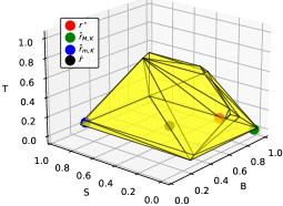
Figure 2: The feasible set with $r^{\star}$ and $\widehat{r},\widehat{r}_{M,K},\widehat{r}_{m,K}$. Axis $B,S,T$ refer to the reward values of B, S and T.

6 Discussion on Model Selection

In this section, we provide some considerations on model selection that use the representation of feedback through two components presented in Section 3. For simplicity of presentation, we consider a single feedback $\mathcal{F}=\{f\}$, with $f=(\mathcal{D},\mathbb{A})$, and we assume that infinite data are available.

Modelling feedback.  In practical applications, we observe the data $\mathcal{D}$, and we have to select the assumption $\mathbb{A}$ based on our knowledge on how $\mathcal{D}$ has been generated.

Example 6.1 (Feedback of driving safely).

Let the unknown target reward $r^{\star}$ represent the task of driving safely. Let $\mathcal{D}=\{\omega_{i}\}_{i}$ be a dataset of demonstrations collected by an agent $\pi^{E}$ that “aims to demonstrate how to drive safely in a certain environment”. What assumption do we adopt?

We can decide to model the problem in different ways, i.e., there are always multiple assumptions $\mathbb{A}$ that can be associated to the given data $\mathcal{D}$ to try to capture the “true” relationship between $\mathcal{D}$ and the underlying unknown $r^{\star}$.

Example 6.1 (continue). We can model $\pi^{E}$ as an optimal policy for the “driving safely” task by using assumption $\mathbb{A}^{\text{OPT}}$ (see Example 3.5). If we think that the demonstrated $\pi^{E}$ sometimes takes suboptimal actions, then we might prefer using $\mathbb{A}^{\text{MCE}}$. Alternatively, we can simply assume that $\pi^{E}$ is at least $\epsilon$-optimal for some $\epsilon>0$, i.e., $J^{\pi^{E}}(r^{\star};p)\geq J^{*}(r^{\star};p)-\epsilon$. We call this assumption $\mathbb{A}^{\text{SUB}}$.

We incur in misspecification if $\mathbb{A}$ does not correctly describe the relationship between $r^{\star}$ and $\mathcal{D}$ (see Skalse & Abate (2024) for an analysis of misspecification in IRL).

Example 6.1 (continue). If we model data $\mathcal{D}$ using assumption $\mathbb{A}^{\text{MCE}}$, but, actually, $\pi^{E}$ is optimal (i.e., it follows $\mathbb{A}^{\text{OPT}}$), then our feedback is misspecified.

Choosing the correct modelling assumption.  The crucial question is: what is the best modelling assumption for the given data $\mathcal{D}$? Intuitively, any assumption that permits to carry out the downstream ReL application $g$ effectively is satisfactory. In other words, we can tolerate some misspecification error as long as the final outcome is acceptable.
Thanks to our framework, we can make these considerations more quantitative. As explained in Section 4, the (non)informativeness $\overline{\mathcal{I}}_{\{f\},g}$ represents the minimum error that can be achieved in the worst-case for doing $g$ using $f=(\mathcal{D},\mathbb{A})$. Under the model of feedback $f$ (i.e., the assumption $\mathbb{A}$) considered, the worst-case error cannot be smaller than $\overline{\mathcal{I}}_{\{f\},g}$. Therefore, this is unsatisfactory if we aim to carry out $g$ with an error $\Delta<\overline{\mathcal{I}}_{\{f\},g}$.
To solve this issue, we have to reduce the size of the feasible set $\mathcal{R}_{f}$ so that its Chebyshev radius $\overline{\mathcal{I}}_{\{f\},g}$ reduces too. There are two ways for doing this. The best one $(i)$ consists in collecting additional feedback $f^{\prime}$ to obtain $\mathcal{R}_{f}\cap\mathcal{R}_{f^{\prime}}\subseteq\mathcal{R}_{f}$ (e.g., through active learning, see Appendix D). However, additional feedback might not be available in practice. The other way $(ii)$ consists in imposing “more structure” to the problem by changing the assumption $\mathbb{A}$ to $\mathbb{A}^{\prime}$ to restrict the feasible set $\mathcal{R}_{\{\mathcal{D},\mathbb{A}\}}$ to $\mathcal{R}_{\{\mathcal{D},\mathbb{A}^{\prime}\}}$.

Example 6.2.

If we model $\mathcal{D}$ using $\mathbb{A}^{\text{OPT}}$, we obtain a feasible set that is strictly contained into the feasible set obtained using assumption $\mathbb{A}^{\text{SUB}}$. Thus, whatever the application $g$ at stake, $\overline{\mathcal{I}}_{\{\mathcal{D},\mathbb{A}^{\text{OPT}}\},g}\leq\overline{\mathcal{I}}_{\{\mathcal{D},\mathbb{A}^{\text{SUB}}\},g}$.

By adopting a more restrictive (less realistic) model $\mathbb{A}^{\prime}$, we reduce the “measurable” error $\overline{\mathcal{I}}_{\{\mathcal{D},\mathbb{A}^{\prime}\},g}$ at the price of a larger unknown misspecification error. This is fine as long as $\mathbb{A}^{\prime}$ is perceived as sufficiently realistic. If there is no realistic assumption with a small enough value of informativeness, then we conclude that the application $g$ cannot be carried out effectively with the only data $\mathcal{D}$. In other words, the ReL problem cannot be solved with the desired accuracy.

7 Related Work

The framework of Skalse et al. (2023b) permits to understand under which conditions the baseline error $D_{\mathcal{F},g}$ is exactly zero, but it does not reveal that some rewards are better than others. Skalse et al. (2023a) quantify the distance between rewards but independently of the application $g$.
To cope with partial identifiability, Amin & Singh (2016); Cao et al. (2021); Kim et al. (2021) assume the availability of a various amount of feedback to reduce the size of the feasible set. Metelli et al. (2021, 2023); Lazzati et al. (2024b, a) circumvent the issue by learning the entire feasible set, postponing the reward selection.
Ziebart et al. (2008); Wulfmeier et al. (2016); Christiano et al. (2017); Ho & Ermon (2016) choose a reward arbitrarily from the feasible set, and this is acceptable for the applications that they consider, but potentially not for others. Ng & Russell (2000); Ratliff et al. (2006); Ramachandran & Amir (2007) make a choice of reward meaningful for the IL application only. In particular, the reward choice $r^{\text{BIRL}}_{\mathcal{F},g}$ of Ramachandran & Amir (2007) can be interpreted in our framework as the minimization of the average “error”:

However, this does not provide any worst-case guarantee.
We mention Ho & Ermon (2016); Zhu et al. (2023) because, for specific applications, as explained in Appendix C.3, their algorithms bypass the computation of a reward and make a robust choice of policy analogous to our reward choice.

8 Conclusion

In this paper, we have presented a novel ReL framework for characterizing the partial identifiability in a quantitative way. We have shown that there exists a robust reward choice that, depending on the application, outperforms all the others in the worst case. Finally, we have illustrated its power in a use case, by providing also provably-efficient algorithms.

Future directions.  We hope that the proposed framework, by enhancing the understanding of ReL problems, will help to improve the performance of ReL algorithms in applications beyond IL and reward design.

Appendix A Additional Results and Proofs for Section 3

In this appendix, we first provide additional explanations and motivations for the “comparisons” feedback, and then we report the missing proofs for Section 3.

A.1 More on the Comparisons Feedback

In the IRL literature, we are given a dataset of demonstrations, i.e., trajectories $\mathcal{D}=\{\omega_{i}\}_{i}\sim d^{p,\pi^{E}}$ collected by executing some (expert) policy $\pi^{E}$ in environment $p$. This setting models the situation in which we observe an agent doing a task many times, and the assumption is that the agent behavior is guided by the reward $r^{\star}$.

In the PbRL literature, we are given two trajectories and a preference signal between them. This setting models the situation in which an agent expresses a preference between two trajectories, i.e., the agent observes two trajectories and says which one it prefers. In doing so, the choice is guided by the target reward $r^{\star}$.

The comparisons feedback introduced in Section 3.2 concerns the scenario in which we have an expert agent (i.e., the agent with $r^{\star}$ in mind) that expresses a preference between two datasets of demonstrations collected by, for instance, other agents. For example, assume that we observe two agents $A_{1},A_{2}$ demonstrating the task of driving a car, and they provide two datasets of demonstrations $\mathcal{D}_{1}=\{\omega^{1}_{i}\}_{i}\sim d^{p,\pi^{1}},\mathcal{D}_{2}=\{\omega^{2}_{i}\}_{i}\sim d^{p,\pi^{2}}$ where $\pi^{1}$ is the policy of $A_{1}$ and $\pi^{2}$ is the policy of $A_{2}$. Assume that we do not want to learn the reward function that guides the behavior of $A_{1}$ nor $A_{2}$, but we aim to learn the reward of a third agent $E$ (i.e., $r^{\star}$ is the reward of $E$). Thus, we can ask to $E$ a preference signal between the behavior of $A_{1},A_{2}$. For instance, we show to $E$ the video of how $A_{1},A_{2}$ drive, and we ask him who drives better. Then, we can use this feedback to infer $r^{\star}$.

A.2 Missing Proofs

See 3.1

Proof.

It is immediate that, for any transition model $p\in\Delta_{\mathcal{S}}\times\mathcal{A}\times\llbracket H\rrbracket^{\mathcal{S}}$ and distribution $\rho\in\Delta^{\mathcal{S}}$, the distances $d_{\text{PL},p},d_{\text{CO},p},d_{\text{GR},\rho}$ are non-negative for any pair of rewards $r,r^{\prime}\in\mathfrak{R}$, and also that they are all 0 when $r=r^{\prime}$. Thus, we conclude that they are premetrics.

Now, consider the identity of indiscernibles property (see Section 2). Given distance $d_{g}$, it does not hold if there exist $r\neq r^{\prime}$ s.t. $d_{g}(r;r^{\prime})=0$. Concerning $d_{\text{PL},p}$, we see that any pair of rewards $r,r^{\prime}$ such that $\Pi^{*}(r;p)=\Pi^{*}(r^{\prime};p)$ satisfies $d_{\text{PL},p}(r,r^{\prime})=0$. Thus, we can take $r^{\prime}$ to be, e.g., a multiple of $r$ to get $d_{\text{PL},p}(r,r^{\prime})=0$. Concerning $d_{\text{CO},p}$, simply consider as $p$ a transition model for which there exists at least a $(s,a,h)\in\mathcal{S}\times\mathcal{A}\times\llbracket H\rrbracket$ s.t., for all $\pi\in\Delta_{\mathcal{S}\times\llbracket H\rrbracket}^{\mathcal{S}}$, $d^{p,\pi}_{h}(s,a)=0$. Then, such triple does not contribute to the performance of any policy, and therefore any pair of rewards $r,r^{\prime}$ that coincide everywhere except for $s,a,h$ satisfy $d_{\text{CO},p}(r,r^{\prime})=0$. Concerning $d_{\text{GR},\rho}$, we can take $r,r^{\prime}$ for which there exists a state $s\in\mathcal{S}$ where $\max_{a\in\mathcal{A}}r(s,a)=\max_{a\in\mathcal{A}}r^{\prime}(s,a)$, but the maximum is achieved by different actions $\operatorname*{arg\,max}_{a\in\mathcal{A}}r(s,a)\neq\operatorname*{arg\,max}_{a\in\mathcal{A}}r^{\prime}(s,a)$. Clearly, $r\neq r^{\prime}$, but $d_{\text{GR},\rho}=0$.

Consider now the simmetry property. For $d_{\text{PL},p}$, take two rewards $r,r^{\prime}$ such that $\Pi^{*}(r;p)=\{\pi^{1}\},\Pi^{*}(r^{\prime};p)=\{\pi^{1},\pi^{2}\}$ for some policies $\pi^{1},\pi^{2}$. Then:

$$d_{\text{PL},p}(r;r^{\prime})\coloneqq J^{*}(r^{\prime};p)-\min\limits_{\pi\in\Pi^{*}(r;p)}J^{\pi}(r^{\prime};p)=J^{\pi^{1}}(r^{\prime};p)-J^{\pi^{1}}(r^{\prime};p)=0,$$

$$d_{\text{PL},p}(r^{\prime};r)\coloneqq J^{*}(r;p)-\min\limits_{\pi\in\Pi^{*}(r^{\prime};p)}J^{\pi}(r;p)=J^{\pi^{1}}(r;p)-J^{\pi^{2}}(r;p)\neq 0.$$

Thus, $d_{\text{PL},p}(r;r^{\prime})\neq d_{\text{PL},p}(r^{\prime};r)$, so simmetry does not hold. For $d_{\text{CO},p}$ the simmetry property holds for any pair of rewards $r,r^{\prime}\in\mathfrak{R}$:

$$d_{\text{CO},p}(r;r^{\prime}) \coloneqq\max_{\pi}\big{|}J^{\pi}(r^{\prime};p)-J^{\pi}(r;p)\big{|}$$

$$=\max_{\pi}\big{|}-\big{(}J^{\pi}(r;p)-J^{\pi}(r^{\prime};p)\big{)}\big{|}$$

$$=\max_{\pi}\big{|}J^{\pi}(r;p)-J^{\pi}(r^{\prime};p)\big{|}$$

$$=d_{\text{CO},p}(r^{\prime};r).$$

Concerning $d_{\text{GR},\rho}$, the simmetry property does not hold. To see it, consider a problem with a single state $s$ and two actions $a_{1},a_{2}$, and let $r,r^{\prime}$ be two rewards such that:

$$r(s,a)=\begin{cases}1&\text{if }a=a_{1},\\ 0&\text{if }a=a_{2},\end{cases},\qquad r^{\prime}(s,a)=\begin{cases}0&\text{if }a=a_{1},\\ 0.5&\text{if }a=a_{2},\end{cases}.$$

Then, we have that:

$$d_{\text{GR},\rho}(r;r^{\prime})\coloneqq\mathbb{E}_{s\sim\rho}\big{[}\max_{a\in\mathcal{A}}r^{\prime}(s,a)-r^{\prime}(s,\pi^{\text{greedy}}(s;r))\big{]}=r^{\prime}(s,a_{2})-r^{\prime}(s,a_{1})=0.5,$$

$$d_{\text{GR},\rho}(r^{\prime};r)\coloneqq\mathbb{E}_{s\sim\rho}\big{[}\max_{a\in\mathcal{A}}r(s,a)-r(s,\pi^{\text{greedy}}(s;r^{\prime}))\big{]}=r(s,a_{1})-r(s,a_{2})=1.$$

Finally, let us consider the triangle inequality property. First, we consider $d_{\text{PL},p}$. Let $r,r^{\prime},r^{\prime\prime}\in\mathfrak{R}$ be three rewards such that $\Pi^{*}(r;p)=\Pi^{*}(r^{\prime\prime};p)=\{\pi_{1}\},\Pi^{*}(r^{\prime};p)=\{\pi^{2}\}$, and take $r^{\prime\prime}=0.5r$. Then:

$$d_{\text{PL},p}(r^{\prime};r)=J^{\pi^{1}}(r;p)-J^{\pi^{2}}(r;p),$$

$$d_{\text{PL},p}(r^{\prime};r^{\prime\prime})=J^{\pi^{1}}(r^{\prime\prime};p)-J^{\pi^{2}}(r^{\prime\prime};p)=0.5J^{\pi^{1}}(r;p)-0.5J^{\pi^{2}}(r;p)=0.5d_{\text{PL},p}(r^{\prime};r),$$

$$d_{\text{PL},p}(r^{\prime\prime};r)=J^{\pi^{1}}(r;p)-J^{\pi^{1}}(r;p)=0.$$

Therefore, we have that:

$$d_{\text{PL},p}(r^{\prime};r)>d_{\text{PL},p}(r^{\prime};r^{\prime\prime})+d_{\text{PL},p}(r^{\prime\prime};r),$$

which proves that triangle inequality does not hold. Concerning $d_{\text{CO},p}$, triangle inequality holds for any $p$ and $r,r^{\prime},r^{\prime\prime}\in\mathfrak{R}$:

$$d_{\text{CO},p}(r^{\prime};r) \coloneqq\max_{\pi}\big{|}J^{\pi}(r;p)-J^{\pi}(r^{\prime};p){\color[rgb]{0,0,1}\pm J^{\pi}(r^{\prime\prime};p)}\big{|}$$

$$\leq\max_{\pi}\big{|}J^{\pi}(r^{\prime\prime};p)-J^{\pi}(r^{\prime};p)|+\max_{\pi}\big{|}J^{\pi}(r;p)-J^{\pi}(r^{\prime\prime};p)|$$

$$=d_{\text{CO},p}(r^{\prime};r^{\prime\prime})+d_{\text{CO},p}(r^{\prime\prime};r),$$

where we have applied the triangle inequality of the absolute value and the fact that the maximum of a sum is smaller than the sum of maxima. As far as $d_{\text{GR},\rho}$ is concerned, we note that it lacks the triangle inequality property with a counterexample analogous to that for $d_{\text{PL},p}$. Consider a problem with a single state $s$ (or $\rho$ supported only on it) and two actions $a_{1},a_{2}$, and consider the rewards $r,r^{\prime},r^{\prime\prime}\in\mathfrak{R}$ such that:

$$r(s,a)=\begin{cases}1&\text{if }a=a_{1},\\ 0&\text{if }a=a_{2},\end{cases},\qquad r^{\prime}(s,a)=\begin{cases}0&\text{if }a=a_{1},\\ 1&\text{if }a=a_{2},\end{cases},\qquad r^{\prime\prime}(s,a)=\begin{cases}0.5&\text{if }a=a_{1},\\ 0&\text{if }a=a_{2},\end{cases}.$$

Then, we have that:

$$d_{\text{GR},\rho}(r^{\prime};r)=r(s,a_{1})-r(s,a_{1})=1,$$

$$d_{\text{GR},\rho}(r^{\prime};r^{\prime\prime})=r^{\prime\prime}(s,a_{1})-r^{\prime\prime}(s,a_{1})=0.5=0.5d_{\text{GR},\rho}(r^{\prime};r),$$

$$d_{\text{GR},\rho}(r^{\prime\prime};r)=r(s,a_{1})-r(s,a_{1})=0.$$

Thus:

$$d_{\text{GR},\rho}(r^{\prime};r)=1>d_{\text{GR},\rho}(r^{\prime};r^{\prime\prime})+d_{\text{GR},\rho}(r^{\prime\prime};r)=0.5+0.$$

This concludes the proof.

∎

Appendix B Additional Results and Proofs for Section 4

In this appendix, we begin by explaining what is the best reward choice in case of multiple feedback for a single application (Section B.1), then we provide the missing proofs for Section 4 (Section B.2).

B.1 The Robust Reward Choice for Multiple Feedback

Consider the setting in which we have an application $g$, and some sets of feedback $\mathcal{F}_{1},\mathcal{F}_{2},\dotsc$ associated to different target rewards $r_{1}^{\star},r_{2}^{\star},\dotsc$, i.e., $r_{1}^{\star}\in\mathcal{R}_{\mathcal{F}_{1}},r_{2}^{\star}\in\mathcal{R}_{\mathcal{F}_{2}},$ and so on. Assume that the rewards $\{r_{i}^{\star}\}_{i}$ are equivalent for $g$, i.e., for any $i,j$, we have: $d_{g}(r^{\star}_{i};r^{\star}_{j})=0$. To make sense of all this information, we can select the set of feedback $\mathcal{F}_{i}$ that reduces the most the worst-case error for $g$, the best way is to select the most “informative” set of feedback $\mathcal{F}_{i}$ for $g$, and then compute the robust reward choice w.r.t. it. Formally, we take index $j\in\operatorname*{arg\,min}_{i}\min_{r\in\mathfrak{R}}\overline{\mathcal{C}}_{\mathcal{F}_{i},g}(r)$, and then we compute $r_{\mathcal{F}_{j},g}$.

B.2 Missing Proofs

See 4.1

Proof.

It is immediate from Assumption 3.1 that $d_{g}(r;r^{\star})$ belongs to the interval. We now show that, if there is an interval smaller than

$$\Big{[}\min\limits_{r^{\prime}\in\mathcal{R}_{\mathcal{F}}}d_{g}(r;r^{\prime}),\max\limits_{r^{\prime}\in\mathcal{R}_{\mathcal{F}}}d_{g}(r;r^{\prime})\Big{]},$$

then it might not contain $r^{\star}$. For simplicity, we prove the result only for the upper bound, because the proof for the lower bound is analogous.

Let $\mathcal{R}_{\mathcal{F}}$ be the feasible set and let $d_{g}$ be a premetric. Assume that Assumption 3.1 holds, i.e., $r^{\star}\in\mathcal{R}_{\mathcal{F}}$, and that no other information on $r^{\star}$ is known. By contradiction, assume that there is an upper bound $U(r,\mathcal{F},d_{g})<\max_{r^{\prime}\in\mathcal{R}_{\mathcal{F}}}d_{g}(r;r^{\prime})$ strictly smaller than $\max_{r^{\prime}\in\mathcal{R}_{\mathcal{F}}}d_{g}(r;r^{\prime})$, and such that $d_{g}(r;r^{\star})\leq U(r,\mathcal{F},d_{g})$. However, since $U(r,\mathcal{F},d_{g})$ does not depend on $r^{\star}$, that can vary freely inside $\mathcal{R}_{\mathcal{F}}$, then we can set $r^{\star}\in\operatorname*{arg\,max}_{r^{\prime}\in\mathcal{R}_{\mathcal{F}}}d_{g}(r;r^{\prime})$. This entails both that $d_{g}(r;r^{\star})\leq U(r,\mathcal{F},d_{g})$ and $U(r,\mathcal{F},d_{g})<\max_{r^{\prime}\in\mathcal{R}_{\mathcal{F}}}d_{g}(r;r^{\prime})=d_{g}(r;r^{\star})$, which is a contradiction. Thus, the claim of the proposition follows. ∎

See 4.2

Proof.

Consider a simple MDP without reward with a single state $s$, three actions $a_{1},a_{2},a_{3}$, and horizon $H=1$. Let $\pi^{1},\pi^{2},\pi^{3}$ be, respectively, the deterministic policies that play actions $a_{1},a_{2},a_{3}$. In this context, take $d_{g}=d_{\text{PL},p}$, and $\mathcal{R}_{\mathcal{F}}=\{r,r^{\prime}\}$, where:

$$r(s,a)=\begin{cases}1&\text{if }a=a_{1},\\ 0&\text{if }a=a_{2},\\ 0.5&\text{if }a=a_{3},\end{cases},\qquad r^{\prime}(s,a)=\begin{cases}0&\text{if }a=a_{1},\\ 1&\text{if }a=a_{2},\\ 0.5&\text{if }a=a_{3},\end{cases}.$$

Since $\Pi^{*}(r;p)=\{\pi^{1}\}$ and $\Pi^{*}(r^{\prime};p)=\{\pi^{2}\}$, then it is immediate that:

$$d_{\text{PL},p}(r;r^{\prime})=d_{\text{PL},p}(r^{\prime};r)=1.$$

The robust reward choice is any reward $r_{\mathcal{F},g}$ s.t. $\Pi^{*}(r_{\mathcal{F},g};p)=\{\pi^{3}\}$. Indeed, in this manner:

$$d_{\text{PL},p}(r_{\mathcal{F},g};r)=d_{\text{PL},p}(r_{\mathcal{F},g};r^{\prime})=0.5.$$

Thus, $r_{\mathcal{F},g}\notin\mathcal{R}_{\mathcal{F}}$. This concludes the proof. ∎

Remark B.1.

The example for Proposition 4.2 can be made also using a convex set $\mathcal{R}_{\mathcal{F}}$. Indeed, if we consider the same example but using as $\mathcal{R}_{\mathcal{F}}$ the convex hull of $r,r^{\prime}$, it is simple to see that no reward in this new feasible set can make $\pi^{3}$ be the unique optimal policy. As such, the Chebyshev center is still external to $\mathcal{R}_{\mathcal{F}}$.

See 4.3

Proof.

Let $(r_{1},r_{2})\in\operatorname*{arg\,max}_{r,r^{\prime}}d_{g}(r;r^{\prime})$, i.e., be the points in the diameter of the feasible set $\mathcal{R}_{\mathcal{F}}$, thus $D_{\mathcal{F},g}=d_{g}(r_{1};r_{2})$. Because of triangle inequality, for any $r\in\mathfrak{R}$ including the Chebyshev center $r_{\mathcal{F},g}$, it holds that:

$$D_{\mathcal{F},g}=d_{g}(r_{1};r_{2}) \leq d_{g}(r_{1};r)+d_{g}(r;r_{2}).$$

If we take $r=r_{\mathcal{F},g}$ and apply simmetry, then we see that $d_{g}(r_{1};r_{\mathcal{F},g})=d_{g}(r_{\mathcal{F},g};r_{1})\leq\max_{r\in\mathcal{R}_{\mathcal{F}}}d_{g}(r_{\mathcal{F},g};r)=\overline{\mathcal{I}}_{\mathcal{F},g}$, and also that $d_{g}(r_{\mathcal{F},g};r_{2})\leq\max_{r\in\mathcal{R}_{\mathcal{F}}}d_{g}(r_{\mathcal{F},g};r)=\overline{\mathcal{I}}_{\mathcal{F},g}$, from which:

$$D_{\mathcal{F},g}=d_{g}(r_{1};r_{2}) \leq 2\overline{\mathcal{I}}_{\mathcal{F},g}.$$

∎

See 4.4

Proof.

The result is immediate by an application of the Jung’s theorem (Jung, 1901; Danzer et al., 1963; Scott, 1991), that states that in every Euclidean space with $n$ dimensions, the Chebyshev radius $r$ of a set with diameter $D$ satisfies:

$$r\leq\sqrt{\frac{n}{2(n+1)}}D.$$

∎

See 4.5

Proof.

Let us begin with $d_{\text{PL},p}$. Consider a problem with horizon $H$ where $\mathcal{R}_{\mathcal{F}}=\{r\in\mathfrak{R}\,|\,\pi_{1}\in\Pi^{*}(r;p)\}$ the feasible set contains all the rewards that make at least $\pi_{1}$ as optimal policy. Consider a transition model $p$ for which there exists a reward $\overline{r}\in\mathcal{R}_{\mathcal{F}}$ s.t. $J^{*}(\overline{r};p)=J^{\pi^{1}}(\overline{r};p)=H$, and for some other policy $\pi^{2}$ it holds that: $J^{\pi^{2}}(\overline{r};p)=0$ (for instance, if we construct $p$ to be deterministic, then, this is possible). Then, since $\mathcal{R}_{\mathcal{F}}$ contains also the reward $r^{\prime}$ that makes all the policies optimal (in particular $\pi^{2}$), we have that:

$$D_{\mathcal{F},(\text{PL},p)}\geq d_{\text{PL},p}(r^{\prime};\overline{r})=J^{*}(\overline{r};p)-J^{\pi^{2}}(\overline{r};p)=H.$$

Instead, if we consider any reward $r^{\prime\prime}$ s.t. $\Pi^{*}(r^{\prime\prime};p)=\{\pi^{1}\}$ (as our robust reward choice), then it is clear that:

$$\overline{\mathcal{I}}_{\mathcal{F},(\text{PL},p)}\leq\max\limits_{r\in\mathcal{R}_{\mathcal{F}}}d_{\text{PL},p}(r^{\prime\prime};r)=J^{*}(r;p)-J^{\pi^{1}}(r;p)=0.$$

The other claim of the proposition can be proved with an analagous construction. ∎

Appendix C Additional Results and Proofs for Section 5

In this appendix, we compute the subgradients of the Lagrangian in Eq. (5) (Section C.1), we provide the missing proofs for Section 5 (Section C.2), we discuss on when the computation of a reward function is necessary in ReL applications by also providing an extension of the proposed framework that bypasses the usage of reward functions (Section C.3), we consider other kinds of feedback (Section C.4), and we provide additional details on the experiments conducted (Section C.5).

It is useful to introduce the following additional notation. Given a trajectory $\omega=\{s_{1},a_{1},\dotsc,s_{H},a_{H},s_{H+1}\}\in\Omega$, we define the state-action visitation distribution of $\omega$ as $d^{\omega}:\mathcal{S}\times\mathcal{A}\times\llbracket H\rrbracket\to\{0,1\}$, so that $d^{\omega}_{h}(s,a)=\mathds{1}\{s=s_{h},a=a_{h}\}$. Moreover, we denote by $\mathbb{R}^{k}_{-}$ the non-positive orthant in $k$ dimensions with $k\geq 1$.

C.1 Subgradients of the Lagrangian

The following quantities are subgradients of the Lagrangian in Eq. (5) evaluated at any $r^{\prime},\lambda^{\prime}\coloneqq[\lambda_{\text{TC}}^{\prime},\lambda_{\text{C}}^{\prime},\lambda_{\text{D}}^{\prime}]$:

$$\partial_{r}\mathcal{L}(r^{\prime},\lambda^{\prime})=(d^{p,\pi^{2}}-d^{p,\pi^{1}})+\sum\nolimits_{i}\lambda_{\text{TC}}^{i,^{\prime}}\big{(}d^{\omega^{1}_{\text{TC},i}}-d^{\omega^{2}_{\text{TC},i}}\big{)}+\sum\nolimits_{i}\lambda_{\text{C}}^{i,^{\prime}}(d^{p_{\text{C},i},\pi^{1}_{\text{C},i}}-d^{p_{\text{C},i},\pi^{2}_{\text{C},i}})$$

$$\qquad\qquad+\sum\nolimits_{i}\lambda_{\text{D}}^{i,^{\prime}}(d^{p_{\text{D},i},\pi^{r^{\prime},*}_{\text{D},i}}-d^{p_{\text{D},i},\pi_{\text{D},i}}),$$

$$\partial_{\lambda^{i}_{\text{TC}}}\mathcal{L}(r^{\prime},\lambda^{\prime})=G(\omega^{1}_{\text{TC},i};r^{\prime})-G(\omega^{2}_{\text{TC},i};r^{\prime}),\qquad\forall i\in\llbracket m_{\text{TC}}\rrbracket$$

$$\partial_{\lambda^{i}_{\text{C}}}\mathcal{L}(r^{\prime},\lambda^{\prime})=J^{\pi^{1}_{\text{C},i}}(r^{\prime};p_{\text{C},i})-J^{\pi^{2}_{\text{C},i}}(r^{\prime};p_{\text{C},i}),\qquad\forall i\in\llbracket m_{\text{C}}\rrbracket$$

$$\partial_{\lambda^{i}_{\text{D}}}\mathcal{L}(r^{\prime},\lambda^{\prime})=J^{*}(r^{\prime};p_{\text{D},i})-J^{\pi_{\text{D},i}}(r^{\prime};p_{\text{D},i})-t_{i},\qquad\forall i\in\llbracket m_{\text{D}}\rrbracket$$

where $\pi^{r^{\prime},*}_{\text{D},i}\in\operatorname*{arg\,max}_{\pi}J^{\pi}(r^{\prime};p_{\text{D},i})$ for all $i\in\llbracket m_{\text{D}}\rrbracket$.

To see it, simply note that the expressions of $\partial_{\lambda^{i}_{\text{TC}}}\mathcal{L},\partial_{\lambda^{i}_{\text{C}}}\mathcal{L},\partial_{\lambda^{i}_{\text{D}}}\mathcal{L}$ are immediate since they are the subgradients of linear functions. Concerning $\partial_{r}\mathcal{L}$, note that the expected utility $J^{\pi^{\prime}}(r^{\prime\prime};p^{\prime})$ under any reward $r^{\prime\prime}$ of any policy $\pi^{\prime}$ in an environment with transition model $p^{\prime}$ is:

$$J^{\pi^{\prime}}(r^{\prime\prime};p^{\prime})=\sum\limits_{(s,a,h)\in\mathcal{S}\times\mathcal{A}\times\llbracket H\rrbracket}d^{p^{\prime},\pi^{\prime}}_{h}(s,a)r_{h}^{\prime\prime}(s,a),$$

and that the return $G(\omega;r^{\prime\prime})$ of any trajectory $\omega$ under $r^{\prime\prime}$ is:

$$G(\omega;r^{\prime\prime})=\sum\limits_{(s,a,h)\in\mathcal{S}\times\mathcal{A}\times\llbracket H\rrbracket}d^{\omega}_{h}(s,a)r_{h}^{\prime\prime}(s,a).$$

Therefore, these (linear) functions are differentiable w.r.t. the reward, and their subgradients coincide with their gradients. All terms of $\partial_{r}\mathcal{L}$ are obtained in this way except for $d^{p_{\text{D},i},\pi^{r^{\prime},*}_{\text{D},i}}$, which is obtained by noticing that $J^{*}(r^{\prime};p_{\text{D},i})=\max_{\pi}J^{\pi}(r^{\prime};p_{\text{D},i})$ is the pointwise maximum of differentiable functions, and thus its subgradient is any convex combination of the gradients of the functions that attain the maximum (Boyd et al., 2022).

C.2 Missing Proofs

C.2.1 Propositions

See 5.1

Proof.

For the (non)compatibility $\overline{\mathcal{C}}_{\mathcal{F},g}(\cdot)$, for any $r\in\mathfrak{R}$, we can write:

$$\overline{\mathcal{C}}_{\mathcal{F},g}(r) \coloneqq\max\limits_{r^{\prime}\in\mathcal{R}_{\mathcal{F}}}d_{g}(r;r^{\prime})$$

$$=\max\limits_{r^{\prime}\in\mathcal{R}_{\mathcal{F}}}\big{|}\Delta J(r)-\Delta J(r^{\prime})\big{|}$$

$$=\max\limits_{r^{\prime}\in\mathcal{R}_{\mathcal{F}}}\max\Big{\{}\Delta J(r)-\Delta J(r^{\prime}),\Delta J(r^{\prime})-\Delta J(r)\Big{\}}$$

$$=\max\Big{\{}\max\limits_{r^{\prime}\in\mathcal{R}_{\mathcal{F}}}\Delta J(r)-\Delta J(r^{\prime}),\max\limits_{r^{\prime}\in\mathcal{R}_{\mathcal{F}}}\Delta J(r^{\prime})-\Delta J(r)\Big{\}}$$

$$=\max\Big{\{}\Delta J(r)-\min\limits_{r^{\prime}\in\mathcal{R}_{\mathcal{F}}}\Delta J(r^{\prime}),\max\limits_{r^{\prime}\in\mathcal{R}_{\mathcal{F}}}\Delta J(r^{\prime})-\Delta J(r)\Big{\}}$$

$$=\max\Big{\{}\Delta J(r)-m,M-\Delta J(r)\Big{\}}.$$

For the diameter $D_{\mathcal{F},g}$, we write:

$$D_{\mathcal{F},g} \coloneqq\max\limits_{r,r^{\prime}\in\mathcal{R}_{\mathcal{F}}}d_{g}(r;r^{\prime})$$

$$=\max\limits_{r,r^{\prime}\in\mathcal{R}_{\mathcal{F}}}\big{|}\Delta J(r)-\Delta J(r^{\prime})\big{|}$$

$$\overset{\textup{\makebox[0.0pt]{(1)}}}{=}\max\limits_{r,r^{\prime}\in\mathcal{R}_{\mathcal{F}}}\big{(}\Delta J(r)-\Delta J(r^{\prime})\big{)}$$

$$=\max\limits_{r\in\mathcal{R}_{\mathcal{F}}}\Delta J(r)-\min\limits_{r^{\prime}\in\mathcal{R}_{\mathcal{F}}}\Delta J(r^{\prime})$$

$$=M-m,$$

where at (1) we note that it cannot be negative, because we can always take $r=r^{\prime}$ which gives 0.

For the informativeness $\overline{\mathcal{I}}_{\mathcal{F},g}$, observe that:

$$\overline{\mathcal{I}}_{\mathcal{F},g} \coloneqq\min_{r\in\mathfrak{R}}\overline{\mathcal{C}}_{\mathcal{F},g}(r)$$

$$=\min_{r\in\mathfrak{R}}\max\Big{\{}\Delta J(r)-m,M-\Delta J(r)\Big{\}},$$

and that the maximum between two quantities is minimized when the two quantities coincide. In this case, when:

$$\Delta J(r)-m=M-\Delta J(r)\quad\iff\quad\Delta J(r)=\frac{M+m}{2}.$$ (10)

Therefore, as long as we can find a reward $r$ such that $\Delta J(r)-m=M-\Delta J(r)$, we know that $\overline{\mathcal{I}}_{\mathcal{F},g}=M-\frac{M+m}{2}=\frac{M+m}{2}-m=\frac{M-m}{2}$. By choosing $r_{\mathcal{F},g}=(r_{M}+r_{m})/2$, i.e.:

$$r_{\mathcal{F},g,h}(s,a)\coloneqq\frac{1}{2}(r_{M,h}(s,a)+r_{m,h}(s,a))\qquad\forall(s,a,h)\in\mathcal{S}\times\mathcal{A}\times\llbracket H\rrbracket,$$

we note that, since by Proposition 5.2 the set $\mathcal{R}_{\mathcal{F}}$ is convex, then $r_{\mathcal{F},g}\in\mathcal{R}_{\mathcal{F}}\subseteq\mathfrak{R}$. Moreover:

$$\overline{\mathcal{C}}_{\mathcal{F},g}(r_{\mathcal{F},g}) =\max\Big{\{}\Delta J(r_{\mathcal{F},g})-m,M-\Delta J(r_{\mathcal{F},g})\Big{\}}$$

$$=\max\Big{\{}\frac{1}{2}\big{(}\Delta J(r_{M})+\Delta J(r_{m})\big{)}-m,M-\frac{1}{2}\big{(}\Delta J(r_{M})+\Delta J(r_{m})\big{)}\Big{\}}$$

$$=\max\Big{\{}\frac{1}{2}\big{(}M+m\big{)}-m,M-\frac{1}{2}\big{(}M+m\big{)}\Big{\}}$$

$$=\max\Big{\{}\frac{M-m}{2},\frac{M-m}{2}\Big{\}}$$

$$=\frac{M-m}{2}.$$

This shows both the claims for $r_{\mathcal{F},g}$ and $\overline{\mathcal{I}}_{\mathcal{F},g}$. ∎

See 5.2

Proof.

The constraints in Eq. (1) and Eq. (2) comprise linear functions of the reward, and thus are convex. Instead, for Eq. (3), the constraints can be rewritten as:

$$J^{*}(r;p_{\text{D},i})-J^{\pi_{\text{D},i}}(r;p_{\text{D},i})-t_{i}\leq 0\;\iff\;\max\limits_{\pi}\Big{(}J^{\pi}(r;p_{\text{D},i})-J^{\pi_{\text{D},i}}(r;p_{\text{D},i})-t_{i}\Big{)}\leq 0,$$

which is the pointwise maximum of convex (linear) functions, and thus it is convex (Boyd & Vandenberghe, 2004).

Since $\mathcal{R}_{\mathcal{F}_{\text{TC}}},\mathcal{R}_{\mathcal{F}_{\text{C}}},\mathcal{R}_{\mathcal{F}_{\text{D}}}$ are all convex, and $\mathcal{R}_{\mathcal{F}}$ is their intersection, then $\mathcal{R}_{\mathcal{F}}$ is convex as well (Boyd & Vandenberghe, 2004). ∎

See 5.6

Proof.

As shown in the proof of Proposition 5.1 in Eq. (10), reward $r_{\mathcal{F},g}$ satisfies this property. ∎

C.2.2 Proof of Theorem 5.5

We begin by writing explicitly the Lagrangian function of the estimated problem, along with its subgradients.

For any ${r}\in\mathfrak{R}$ and ${\lambda}_{\text{TC}}\in\mathbb{R}^{m_{\text{TC}}}_{+},{\lambda}_{\text{C}}\in\mathbb{R}^{m_{\text{C}}}_{+},{\lambda}_{\text{D}}\in\mathbb{R}^{m_{\text{D}}}_{+}$, the Lagrangian $\widehat{\mathcal{L}}$ of both problems in Eq. (8) is (we set ${\lambda}\coloneqq[{\lambda}_{\text{TC}},{\lambda}_{\text{C}},{\lambda}_{\text{D}}]$):

$$\widehat{\mathcal{L}}({r},{\lambda}) =\Delta J(r)+\sum\nolimits_{i}{\lambda}_{\text{TC}}^{i}\big{(}G(\omega^{1}_{\text{TC},i};{r})-G(\omega^{2}_{\text{TC},i};{r})\big{)}+\sum\nolimits_{i}{\lambda}_{\text{C}}^{i}\big{(}\widehat{J}_{{\text{C},i,1}}({r})-\widehat{J}_{{\text{C},i,2}}({r})\big{)}$$

$$+\sum\nolimits_{i}{\lambda}_{\text{D}}^{i}\big{(}J^{*}({r};\widehat{p}_{\text{D},i})-\widehat{J}_{{\text{D},i}}({r})-t_{i}\big{)}.$$ (11)

Similarly to the calculations in Appendix C.1, we can compute the subgradients of this Lagrangian evaluated at any $r^{\prime},\lambda^{\prime}\coloneqq[\lambda_{\text{TC}}^{\prime},\lambda_{\text{C}}^{\prime},\lambda_{\text{D}}^{\prime}]$ as:

$$\begin{split}&\partial_{r}\mathcal{L}(r^{\prime},\lambda^{\prime})=(d^{p,\pi^{2}}-d^{p,\pi^{1}})+\sum\nolimits_{i}\lambda_{\text{TC}}^{i,^{\prime}}\big{(}d^{\omega^{1}_{\text{TC},i}}-d^{\omega^{2}_{\text{TC},i}}\big{)}+\sum\nolimits_{i}\lambda_{\text{C}}^{i,^{\prime}}(\widehat{d}^{\text{C},i,1}-\widehat{d}^{\text{C},i,2})\\ &\qquad\qquad+\sum\nolimits_{i}\lambda_{\text{D}}^{i,^{\prime}}(d^{\widehat{p}_{\text{D},i},\widehat{\pi}^{r^{\prime},*}_{\text{D},i}}-\widehat{d}^{\text{D},i}),\\ &\partial_{\lambda^{i}_{\text{TC}}}\mathcal{L}(r^{\prime},\lambda^{\prime})=G(\omega^{1}_{\text{TC},i};r^{\prime})-G(\omega^{2}_{\text{TC},i};r^{\prime}),\qquad\forall i\in\llbracket m_{\text{TC}}\rrbracket\\ &\partial_{\lambda^{i}_{\text{C}}}\mathcal{L}(r^{\prime},\lambda^{\prime})=\widehat{J}_{{\text{C},i,1}}(r^{\prime})-\widehat{J}_{{\text{C},i,2}}(r^{\prime}),\qquad\forall i\in\llbracket m_{\text{C}}\rrbracket\\ &\partial_{\lambda^{i}_{\text{D}}}\mathcal{L}(r^{\prime},\lambda^{\prime})=J^{*}(r^{\prime};\widehat{p}_{\text{D},i})-\widehat{J}_{{\text{D},i}}(r^{\prime})-t_{i},\qquad\forall i\in\llbracket m_{\text{D}}\rrbracket\end{split}$$ (12)

where $\widehat{\pi}^{r^{\prime},*}_{\text{D},i}\in\operatorname*{arg\,max}_{\pi}J^{\pi}(r^{\prime};\widehat{p}_{\text{D},i})$ for all $i\in\llbracket m_{\text{D}}\rrbracket$.

To prove Theorem 5.5, we have to bound the estimation error and the approximation error. To obtain these bounds, we first have to show that strong duality holds for both the true and the estimated problems.

Lemma C.1.

Under Assumption 5.1, it holds that:

$$M=\min\limits_{\lambda\in\mathfrak{D}_{+}}\max\limits_{r\in\mathfrak{R}}\mathcal{L}(r,\lambda),$$

$$m=\max\limits_{\lambda\in\mathfrak{D}_{-}}\min\limits_{r\in\mathfrak{R}}\mathcal{L}(r,\lambda),$$

where $\mathfrak{D}_{+}=\{\lambda\in\mathbb{R}_{+}^{|\mathcal{F}|}\,|\,\|\lambda\|_{1}\leq 2H/\xi\}$ and $\mathfrak{D}_{-}=\{\lambda\in\mathbb{R}_{-}^{|\mathcal{F}|}\,|\,\|\lambda\|_{1}\leq 2H/\xi\}$.

Proof.

Under Assumption 5.1, we have that Slater’s constraint qualification holds. Thanks also to the linearity of $\Delta J(\cdot)$ and to the convexity of $\mathcal{R}_{\mathcal{F}}$ (see Proposition 5.2), we have that strong duality holds (Boyd & Vandenberghe, 2004), thus:

$$M=\min\limits_{\lambda\in\mathbb{R}^{|\mathcal{F}|}_{+}}\max\limits_{r\in\mathfrak{R}}\mathcal{L}(r,\lambda),$$

$$m=\max\limits_{\lambda\in\mathbb{R}^{|\mathcal{F}|}_{-}}\min\limits_{r\in\mathfrak{R}}\mathcal{L}(r,\lambda).$$

To prove the boundedness of the Lagrange multipliers, let $(r^{*},\lambda^{*})$ be any saddle point for problem $M$ (the proof for $m$ is analagous). Under Assumption 5.1, we can apply Lemma 3 of Nedić & Ozdaglar (2009) to obtain that, for the reward $\overline{r}$ in Assumption 5.1:

$$\|\lambda^{*}\|_{1} \leq\frac{\Delta J(\overline{r})-M}{\xi}$$

$$\leq\frac{\Delta J(\overline{r})+H}{\xi}$$

$$\leq\frac{2H}{\xi}.$$

Thus, the values of the Lagrange multipliers in saddle points can be found in $\mathfrak{D}_{+}\subset\mathbb{R}_{+}^{|\mathcal{F}|}$. An analagous reasoning can be applied for $m$. ∎

To prove that strong duality holds for the estimated problem, we have to enforce the Slater’s constraint qualification to hold with high probability. To do so, the following lemma proves useful:

Lemma C.2 (Concentration).

Let $\epsilon_{\text{EST}}\in(0,1),\delta\in(0,1)$, and define events:

$$\begin{split}&\mathcal{E}_{C,1}\coloneqq\Big{\{}\sup\limits_{r\in\mathfrak{R}}\Big{|}\widehat{J}_{{\text{C},i,1}}({r})-J^{\pi^{1}_{\text{C},i}}(r;p_{\text{C},i})\Big{|}\leq\epsilon_{\text{EST}}/2\quad\forall i\in\llbracket m_{\text{C}}\rrbracket\Big{\}},\\ &\mathcal{E}_{C,2}\coloneqq\Big{\{}\sup\limits_{r\in\mathfrak{R}}\Big{|}\widehat{J}_{{\text{C},i,2}}({r})-J^{\pi^{2}_{\text{C},i}}(r;p_{\text{C},i})\Big{|}\leq\epsilon_{\text{EST}}/2\quad\forall i\in\llbracket m_{\text{C}}\rrbracket\Big{\}},\\ &\mathcal{E}_{D}\coloneqq\Big{\{}\sup\limits_{r\in\mathfrak{R}}\Big{|}\widehat{J}_{{\text{D},i}}({r})-J^{\pi_{\text{D},i}}(r;p_{\text{D},i})\Big{|}\leq\epsilon_{\text{EST}}/2\quad\forall i\in\llbracket m_{\text{D}}\rrbracket\Big{\}},\\ &\mathcal{E}_{D,*}\coloneqq\Big{\{}\sup\limits_{r\in\mathfrak{R}}\Big{|}J^{*}({r};\widehat{p}_{\text{D},i})-J^{*}(r;p_{\text{D},i})\Big{|}\leq\epsilon_{\text{EST}}/2\quad\forall i\in\llbracket m_{\text{D}}\rrbracket\Big{\}}.\end{split}$$ (13)

Then, the good event $\mathcal{E}\coloneqq\mathcal{E}_{\text{C,1}}\cap\mathcal{E}_{\text{C,1}}\cap\mathcal{E}_{\text{D}}\cap\mathcal{E}_{\text{D},*}$ holds with probability at least $1-\delta$, with at most:

$$\begin{split}&n^{1}_{\text{C},i},n^{2}_{\text{C},i},n_{\text{D},i}\leq\widetilde{\mathcal{O}}\Big{(}\frac{SAH^{3}}{\epsilon_{\text{EST}}}\log\frac{m_{\text{C}}+m_{\text{D}}}{\delta}\Big{)},\\ &N_{\text{D},i}\leq\widetilde{\mathcal{O}}\Big{(}\frac{SAH^{3}}{\epsilon_{\text{EST}}}\Big{(}S+\log\frac{m_{\text{C}}+m_{\text{D}}}{\delta}\Big{)}\Big{)}.\end{split}$$ (14)

Proof.

Our algorithms estimate the visit distribution through their empirical estimates, defined in Eq. (7). Thus, noticing that a bound in 1-norm implies the bound on the difference of the expected utilities under all $r\in\mathfrak{R}$, as shown in the proof of Theorem 5.1 of Lazzati et al. (2024a), with probability at least $1-\delta/2$ (we do a union bound), it holds $\mathcal{E}_{\text{C,1}}\cap\mathcal{E}_{\text{C,1}}\cap\mathcal{E}_{\text{D}}$. Then, by using the guarantee in Menard et al. (2021), we have that, with probability at least $1-\delta/2$, $\mathcal{E}_{\text{D},*}$ holds. The result follows by an application of the union bound. ∎

Thanks to this lemma, we know that, with high probability, Slater’s constraint qualification applies also to the estimated problems:

Lemma C.3 (Slater’s Condition).

Let $\delta\in(0,1)$. Under Assumption 5.1, there exists $\xi>0$ and $\overline{r}\in\mathfrak{R}$ such that, if $\epsilon_{\text{EST}}\in(0,\xi/2)$, then, with probability $1-\delta$:

$$\begin{cases}G(\omega^{1}_{\text{TC},i};\overline{r})\leq G(\omega^{2}_{\text{TC},i};\overline{r})-(\xi-\epsilon_{\text{EST}})&\forall i\in\llbracket m_{\text{TC}}\rrbracket\\ \widehat{J}_{{\text{C},i,1}}(\overline{r})\leq\widehat{J}_{{\text{C},i,2}}(\overline{r})-(\xi-\epsilon_{\text{EST}})&\forall i\in\llbracket m_{\text{C}}\rrbracket\\ \widehat{J}_{{\text{D},i}}(\overline{r})\geq\widehat{J}^{*}(\overline{r};\widehat{p}_{\text{D},i})-t_{i}+(\xi-\epsilon_{\text{EST}})&\forall i\in\llbracket m_{\text{D}}\rrbracket\end{cases},$$

with the number of samples in Eq. (LABEL:eq:_sample_complexity_lemma_concentration).

Proof.

The result follows directly by considering the values $\xi,\overline{r}$ in Assumption 5.1, and applying Lemma C.2. For instance, considering the comparison feedback, we have:

$$\widehat{J}_{{\text{C},i,1}}(\overline{r})-\widehat{J}_{{\text{C},i,2}}(\overline{r}) =\widehat{J}_{{\text{C},i,1}}(\overline{r})-\widehat{J}_{{\text{C},i,2}}(\overline{r}){\color[rgb]{0,0,1}\pm\big{(}J^{\pi^{1}_{\text{C},i}}(\overline{r};p_{\text{C},i})-J^{\pi^{2}_{\text{C},i}}(\overline{r};p_{\text{C},i})\big{)}}$$

$$\leq{\color[rgb]{0,0,1}\epsilon_{\text{EST}}}+\big{(}J^{\pi^{1}_{\text{C},i}}(\overline{r};p_{\text{C},i})-J^{\pi^{2}_{\text{C},i}}(\overline{r};p_{\text{C},i})\big{)}$$

$$\leq\epsilon_{\text{EST}}-\xi.$$

∎

Thanks to Lemma C.3, we see that, with high probability, strong duality holds also for the estimated problem, and the Lagrange multipliers are bounded.

Lemma C.4.

Let $\epsilon_{\text{EST}}\in(0,\xi/2),\delta\in(0,1)$. Under Assumption 5.1, with probability $1-\delta$, we have:

$$\widehat{M}=\min\limits_{\lambda\in\widehat{\mathfrak{D}}_{+}}\max\limits_{r\in\mathfrak{R}}\widehat{\mathcal{L}}(r,\lambda),$$

$$\widehat{m}=\max\limits_{\lambda\in\widehat{\mathfrak{D}}_{-}}\min\limits_{r\in\mathfrak{R}}\widehat{\mathcal{L}}(r,\lambda),$$

where $\widehat{\mathfrak{D}}_{+}=\{\lambda\in\mathbb{R}_{+}^{|\mathcal{F}|}\,|\,\|\lambda\|_{1}\leq 4H/\xi\}$ and $\widehat{\mathfrak{D}}_{-}=\{\lambda\in\mathbb{R}_{-}^{|\mathcal{F}|}\,|\,\|\lambda\|_{1}\leq 4H/\xi\}$.

Proof.

The proof is analogous to that of Lemma C.1 using Lemma C.3, by replacing $\xi$ with $\xi-\epsilon_{\text{EST}}\geq\xi/2$. ∎

We are now ready to bound the sample complexity, i.e., the difference between the optimal solutions of the true problem and the estimated problem. See 5.3

Proof.

We proceed for $M,\widehat{M}$ (the proof for $m,\widehat{m}$ is completely analogous):

$$\Big{|}M-\widehat{M}\Big{|} =\Big{|}\min\limits_{\lambda\in\mathfrak{D}_{+}}\max\limits_{r\in\mathfrak{R}}\mathcal{L}(r,\lambda)-\min\limits_{\lambda\in\widehat{\mathfrak{D}}_{+}}\max\limits_{r\in\mathfrak{R}}\widehat{\mathcal{L}}(r,\lambda)\Big{|}$$

$$\overset{\textup{\makebox[0.0pt]{(1)}}}{=}\Big{|}{\color[rgb]{0,0,1}\min\limits_{\lambda\in\widehat{\mathfrak{D}}_{+}}}\max\limits_{r\in\mathfrak{R}}\mathcal{L}(r,\lambda)-\min\limits_{\lambda\in\widehat{\mathfrak{D}}_{+}}\max\limits_{r\in\mathfrak{R}}\widehat{\mathcal{L}}(r,\lambda)\Big{|}$$

$$\overset{\textup{\makebox[0.0pt]{(2)}}}{\leq}{\color[rgb]{0,0,1}\max\limits_{\lambda\in\widehat{\mathfrak{D}}_{+}}}\Big{|}\max\limits_{r\in\mathfrak{R}}\mathcal{L}(r,\lambda)-\max\limits_{r\in\mathfrak{R}}\widehat{\mathcal{L}}(r,\lambda)\Big{|}$$

$$\overset{\textup{\makebox[0.0pt]{(3)}}}{\leq}\max\limits_{\lambda\in\widehat{\mathfrak{D}}_{+}}{\color[rgb]{0,0,1}\max\limits_{r\in\mathfrak{R}}}\Big{|}\mathcal{L}(r,\lambda)-\widehat{\mathcal{L}}(r,\lambda)\Big{|}$$

$$=\max\limits_{\lambda\in\widehat{\mathfrak{D}}_{+}}\max\limits_{r\in\mathfrak{R}}\Big{|}\sum\nolimits_{i}{\lambda}_{\text{C}}^{i}\Big{(}\big{(}\widehat{J}_{{\text{C},i,1}}({r})-\widehat{J}_{{\text{C},i,2}}({r})\big{)}-\big{(}J^{\pi^{1}_{\text{C},i}}(r;p_{\text{C},i})-J^{\pi^{2}_{\text{C},i}}(r;p_{\text{C},i})\big{)}\Big{)}$$

$$\qquad+\sum\nolimits_{i}{\lambda}_{\text{D}}^{i}\Big{(}\big{(}J^{*}({r};\widehat{p}_{\text{D},i})-\widehat{J}_{{\text{D},i}}({r})\big{)}-\big{(}J^{*}(r;p_{\text{D},i})-J^{\pi_{\text{D},i}}(r;p_{\text{D},i})\big{)}\Big{)}\Big{|}$$

$$\overset{\textup{\makebox[0.0pt]{(4)}}}{\leq}{\color[rgb]{0,0,1}\epsilon_{\text{EST}}}\max\limits_{\lambda\in\widehat{\mathfrak{D}}_{+}}\|{\lambda}\|_{1}$$

$$\overset{\textup{\makebox[0.0pt]{(5)}}}{\leq}\epsilon_{\text{EST}}{\color[rgb]{0,0,1}\frac{4H}{\xi}},$$

where at (1) we used Lemma C.1 and Lemma C.4, at (2) and at (3) the Lipschitzianity of the maximum operator. At (4) we use Lemma C.2 and we upper bound with the 1-norm of $\lambda$, and at (5) we use the definition of set $\widehat{\mathfrak{D}}_{+}$.

By choosing:

$$\epsilon_{\text{EST}}<\frac{\xi\epsilon}{4H},$$

which is smaller than $\xi/2$ for $\epsilon\in(0,2H]$, we get the result.

∎

To bound the approximation error, we first need to show that the norm of the subgradients is bounded. We denote as $\widehat{\lambda}_{M,k}=[\widehat{\lambda}_{\text{TC},M,k},\widehat{\lambda}_{\text{C},M,k},\widehat{\lambda}_{\text{D},M,k}]$ and $\widehat{\lambda}_{m,k}=[\widehat{\lambda}_{\text{TC},m,k},\widehat{\lambda}_{\text{C},m,k},\widehat{\lambda}_{\text{D},m,k}]$ the Lagrange multipliers computed by the PDSM at iteration $k$, for all $k\geq 0$, for both problems. The method comes from Nedić & Ozdaglar (2009), and is reported in Eq. (6). We apply it to the estimated problem, i.e., to $\widehat{\mathcal{L}}$ with subgradients in Eq. (12).

Lemma C.5.

If we execute the PDSM (Eq. (6)) on the estimated problem (Eq. (8)) starting with arbitrary $\widehat{r}_{M,0}$ (resp. $\widehat{r}_{m,0}$) and $\widehat{\lambda}_{M,0}$ (resp. $\widehat{\lambda}_{m,0}$), and using $\mathfrak{D}=\mathfrak{D}_{\ell,+}\coloneqq\{\lambda\in\mathbb{R}_{+}^{|\mathcal{F}|}\,|\,\|\lambda\|_{2}\leq 4H/\xi+\ell\}$ (resp. $\mathfrak{D}=\mathfrak{D}_{\ell,-}\coloneqq\{\lambda\in\mathbb{R}_{-}^{|\mathcal{F}|}\,|\,\|\lambda\|_{2}\leq 4H/\xi+\ell\}$), with $\ell\geq 0$, then it holds that:

$$\max\limits_{k\in\mathbb{R}_{+}}\max\Big{\{}\|\partial_{r}\widehat{\mathcal{L}}(\widehat{r}_{M,k},\widehat{\lambda}_{M,k})\|_{2},\|\partial_{\lambda}\widehat{\mathcal{L}}(\widehat{r}_{M,k},\widehat{\lambda}_{M,k})\|_{2}\Big{\}}\leq 4\sqrt{H|\mathcal{F}|}\Big{(}\frac{4H}{\xi}+\ell\Big{)}.$$

Proof.

We prove the result for $M$ only, because for $m$ is analogous. Consider the subgradient expressions in Eq. (12). For $\partial_{r}\widehat{\mathcal{L}}$, we can write:

$$\max\limits_{k\in\mathbb{R}_{+}}\|\partial_{r}\widehat{\mathcal{L}}(\widehat{r}_{M,k},\widehat{\lambda}_{M,k})\|_{2} \leq{\color[rgb]{0,0,1}\max\limits_{r^{\prime}\in\mathfrak{R}}\max\limits_{\lambda^{\prime}\in\mathfrak{D}_{\ell,+}}}\|\partial_{r}\widehat{\mathcal{L}}(r^{\prime},\lambda^{\prime})\|_{2}$$

$$=\max\limits_{r^{\prime}\in\mathfrak{R}}\max\limits_{\lambda^{\prime}\in\mathfrak{D}_{\ell,+}}\Big{\|}(d^{p,\pi^{2}}-d^{p,\pi^{1}})+\sum\nolimits_{i}\lambda_{\text{TC}}^{i,^{\prime}}\big{(}d^{\omega^{1}_{\text{TC},i}}-d^{\omega^{2}_{\text{TC},i}}\big{)}+\sum\nolimits_{i}\lambda_{\text{C}}^{i,^{\prime}}(\widehat{d}^{\text{C},i,1}-\widehat{d}^{\text{C},i,2})$$

$$\qquad+\sum\nolimits_{i}\lambda_{\text{D}}^{i,^{\prime}}(d^{\widehat{p}_{\text{D},i},\widehat{\pi}^{r^{\prime},*}_{\text{D},i}}-\widehat{d}^{\text{D},i})\Big{\|}_{2}$$

$$\leq\max\limits_{r^{\prime}\in\mathfrak{R}}\max\limits_{\lambda^{\prime}\in\mathfrak{D}_{\ell,+}}\Big{\|}d^{p,\pi^{2}}-d^{p,\pi^{1}}\Big{\|}_{2}+\sum\nolimits_{i}|\lambda_{\text{TC}}^{i,^{\prime}}|\Big{\|}d^{\omega^{1}_{\text{TC},i}}-d^{\omega^{2}_{\text{TC},i}}\Big{\|}_{2}+\sum\nolimits_{i}|\lambda_{\text{C}}^{i,^{\prime}}|\Big{\|}\widehat{d}^{\text{C},i,1}-\widehat{d}^{\text{C},i,2}\Big{\|}_{2}$$

$$\qquad+\sum\nolimits_{i}|\lambda_{\text{D}}^{i,^{\prime}}|\Big{\|}d^{\widehat{p}_{\text{D},i},\widehat{\pi}^{r^{\prime},*}_{\text{D},i}}-\widehat{d}^{\text{D},i}\Big{\|}_{2}$$

$$\overset{\textup{\makebox[0.0pt]{(1)}}}{\leq}{\color[rgb]{0,0,1}2\sqrt{H}}\max\limits_{\lambda^{\prime}\in\mathfrak{D}_{\ell,+}}\big{(}1+\|\lambda^{\prime}\|_{1}\big{)}$$

$$\leq 2\sqrt{H}\Big{(}1+{\color[rgb]{0,0,1}\sqrt{|\mathcal{F}|}}\max\limits_{\lambda^{\prime}\in\mathfrak{D}_{\ell,+}}\|\lambda^{\prime}\|_{{\color[rgb]{0,0,1}2}}\Big{)}$$

$$=2\sqrt{H}\bigg{[}1+\sqrt{|\mathcal{F}|}\Big{(}\frac{4H}{\xi}+\ell\Big{)}\bigg{]}$$

$$\overset{\textup{\makebox[0.0pt]{(2)}}}{\leq}4\sqrt{H|\mathcal{F}|}\Big{(}\frac{4H}{\xi}+\ell\Big{)},$$

where at (1) we use the fact that the 2-norm of every visit distribution is at most $\sqrt{H}$, and at (2) that $H\geq 1$.

By observing that the difference between returns and expected utilities is bounded in $[-H,+H]$, and that $k_{i}\in[0,H]$ for all $i\in\llbracket m\rrbracket_{\text{D}}$, we get that:

$$\max\limits_{k\in\mathbb{R}_{+}}\|\partial_{\lambda}\widehat{\mathcal{L}}(\widehat{r}_{M,k},\widehat{\lambda}_{M,k})\|_{2} \leq{\color[rgb]{0,0,1}\max\limits_{r^{\prime}\in\mathfrak{R}}\max\limits_{\lambda^{\prime}\in\mathfrak{D}_{\ell,+}}}\|\partial_{\lambda}\widehat{\mathcal{L}}(r^{\prime},\lambda^{\prime})\|_{2}$$

$$\leq 2H\sqrt{|\mathcal{F}|},$$

where we used Cauchy-Schwarz inequality. ∎

We can now bound the iteration complexity: See 5.4

Proof.

We prove the result for $M$, because the proof for $m$ is analogous. We work under the good event $\mathcal{E}$ in Lemma C.2, we know that strong duality holds by Lemma C.4, and we know that the subgradients are bounded by Lemma C.5.

Define $L\in\mathbb{R}$ as the upper bound to the norm of the subgradients:

$$L\coloneqq 4\sqrt{H|\mathcal{F}|}\Big{(}\frac{4H}{\xi}+\ell\Big{)},$$

and choose the following values for the hyperparameters:

$$\widehat{r}_{M,0}=\text{arbitrary in }\mathfrak{R},$$

$$\widehat{\lambda}_{M,0}=0,$$

$$\ell=\sqrt{\Big{(}\frac{4H}{\xi}\Big{)}^{2}+\frac{SAH}{4}},$$

$$\alpha=\frac{\epsilon}{2L^{2}}.$$

We can apply Proposition 2 of Nedić & Ozdaglar (2009) to obtain:

$$\widehat{M}_{K}-\widehat{M}\leq\frac{\|\widehat{\lambda}_{M,0}\|_{2}^{2}}{2K\alpha}+\frac{\|\widehat{r}_{M,0}-\widehat{r}_{M}\|_{2}^{2}}{2K\alpha}+\alpha L^{2},$$

$$\widehat{M}-\widehat{M}_{K}\leq\frac{4H}{\xi}\Big{(}\frac{2}{K\alpha\ell}\Big{(}\frac{4H}{\xi}+\ell\Big{)}^{2}+\frac{\|\widehat{r}_{M,0}-\widehat{r}_{M}\|^{2}_{2}}{2K\alpha\ell}+\frac{\alpha L^{2}}{2\ell}\Big{)}.$$

Using the choice of hyperparameters, the first term is bounded as:

$$\widehat{M}_{K}-\widehat{M} \leq\frac{SAH}{2K\alpha}+\alpha L^{2},$$

$$\leq\frac{SAHL^{2}}{\epsilon K}+\frac{\epsilon}{2},$$

which is smaller than $\epsilon$ if:

$$K\geq\frac{SAHL^{2}}{2\epsilon^{2}}.$$

Concerning the second term, we write:

$$\widehat{M}-\widehat{M}_{K} \leq\frac{4H}{\xi}\frac{2}{K\alpha\ell}\Big{(}\frac{4H}{\xi}+\ell\Big{)}^{2}+\frac{4H}{\xi}\frac{SAH}{2K\alpha\ell}+\frac{4H}{\xi}\frac{\alpha L^{2}}{2\ell}$$

$$\overset{\textup{\makebox[0.0pt]{(1)}}}{\leq}\frac{4H}{\xi}\frac{2}{K\alpha\ell}\Big{(}\frac{4H}{\xi}+\ell\Big{)}^{2}+\frac{4H}{\xi}\frac{SAH}{2K\alpha\ell}+{\color[rgb]{0,0,1}\frac{\epsilon}{2}}$$

$$\overset{\textup{\makebox[0.0pt]{(2)}}}{\leq}\frac{4H}{\xi}\frac{2}{K\alpha\ell}\Big{(}\frac{4H}{\xi}+\ell\Big{)}^{2}+\frac{4H}{\xi}{\color[rgb]{0,0,1}\frac{\sqrt{SAH}}{K\alpha}}+{\frac{\epsilon}{2}}$$

$$\overset{\textup{\makebox[0.0pt]{(3)}}}{\leq}\frac{4H}{\xi}\frac{2}{K\alpha}{\color[rgb]{0,0,1}\Big{(}\frac{16H}{\xi}+\frac{\sqrt{SAH}}{2}\Big{)}}+\frac{4H}{\xi}{\frac{\sqrt{SAH}}{K\alpha}}+{\frac{\epsilon}{2}}$$

$$\leq\frac{8H}{\xi}{\frac{\sqrt{SAH}}{K\alpha}}+\frac{128H^{2}}{\xi^{2}K\alpha}+\frac{\epsilon}{2},$$

where at (1) we use that $\ell\geq 2H/\xi$ and the choice of $\alpha$, at (2) we use that $\ell\geq\sqrt{\frac{SAH}{4}}$, at (3) we use that $\Big{(}\frac{4H}{\xi}+\ell\Big{)}^{2}/\ell\leq\frac{16H}{\xi}+\frac{\sqrt{SAH}}{2}$. This quantity is smaller than $\epsilon$ if:

$$\frac{16H^{3/2}L^{2}}{\xi K\epsilon}\Big{(}\sqrt{SA}+\frac{16\sqrt{H}}{\xi}\Big{)}\leq\frac{\epsilon}{2}\quad\iff\quad K\geq\frac{32H^{3/2}L^{2}}{\xi\epsilon^{2}}\Big{(}\sqrt{SA}+\frac{16\sqrt{H}}{\xi}\Big{)}.$$

The result follows by inserting the definition of $L$:

$$K \geq\mathcal{O}\bigg{(}\frac{HL^{2}}{\epsilon^{2}}\max\Big{\{}SA,H\sqrt{SA}/\xi^{2}\Big{\}}\bigg{)}$$

$$\leq\mathcal{O}\bigg{(}\frac{SAH^{2}L^{2}}{\xi^{2}\epsilon^{2}}\bigg{)}.$$

∎

See 5.5

Proof.

The result follows by applying Lemma 5.3 and Lemma 5.4 to the explicit representations of the learning targets in Proposition 5.1. Indeed, through triangle inequality, this guarantees that:

$$\big{|}M-\widehat{M}_{K}\big{|}\leq\epsilon,\quad\wedge\quad\big{|}m-\widehat{m}_{K}\big{|}\leq\epsilon,$$

as long as we rescale $\epsilon\to\epsilon/2$.

Concerning the informativeness and the baseline error, the result is immediate:

$$\Big{|}D_{\mathcal{F},g}-\widehat{D}\Big{|} =\Big{|}M-m-(\widehat{M}_{K}-\widehat{m}_{K})\Big{|}\leq\epsilon.$$

For the compatibility, we write:

$$\sup\limits_{r\in\mathfrak{R}}\Big{|}\overline{\mathcal{C}}_{\mathcal{F},g}(r)-\widehat{\mathcal{C}}(r)\Big{|} =\Big{|}\max\big{\{}M-\Delta J(r),\Delta J(r)-m\big{\}}-\max\big{\{}\widehat{M}_{K}-\Delta J(r),\Delta J(r)-\widehat{m}_{K}\big{\}}\Big{|}$$

$$\leq\max\big{\{}\Big{|}M-\Delta J(r)-(\widehat{M}_{K}-\Delta J(r))\Big{|},\Big{|}\Delta J(r)-m-(\Delta J(r)-\widehat{m}_{K})\Big{|}\big{\}}$$

$$\leq\epsilon.$$

For the robust reward choice, simply note that:

$$\Big{|}\overline{\mathcal{I}}_{\mathcal{F},g}-\overline{\mathcal{C}}_{\mathcal{F},g}(\widehat{r})\Big{|} =\Big{|}\frac{M-m}{2}-\max\big{\{}M-\Delta J(\widehat{r}),\Delta J(\widehat{r})-m\big{\}}\Big{|}$$

$$=\Big{|}\frac{M-m}{2}-\max\big{\{}M-(\widehat{M}_{K}+\widehat{m}_{K})/2,(\widehat{M}_{K}+\widehat{m}_{K})/2-m\big{\}}\Big{|}$$

$$\leq\max\big{\{}\Big{|}\frac{M-m}{2}-M+(\widehat{M}_{K}+\widehat{m}_{K})/2\Big{|},\Big{|}\frac{M-m}{2}-(\widehat{M}_{K}+\widehat{m}_{K})/2+m\big{\}}\Big{|}$$

$$\leq\epsilon.$$

∎

C.3 Bypassing the Need for a Reward Function

All ReL papers make the underlying assumption that the feedback received is “reward-rational” (Jeon et al., 2020), in the sense that there exists a reward function $r^{\star}$ that drives it (see Assumption 3.1). However, the ultimate goal of ReL is not to learn $r^{\star}$, but is to learn some quantity $x$ (that depends on $r^{\star}$). For instance, in IL the goal is to learn a policy (optimal under $r^{\star}$), while in the application considered in Section 5 the final goal is to compute a scalar (the difference in performance under $r^{\star}$ between $\pi^{2}$ and $\pi^{1}$). For this reason, in this section, we ask ourselves whether it is possible to do ReL without explicitly computing any reward, i.e., by directly computing the desired quantity $x$ from the feedback.

We begin by extending the framework and the robust choice presented in Section 3 and Section 4 to the “ReL without reward” problem, and then we argue that there are applications in which this is not possible.

C.3.1 A ReL Framework without Reward Functions

In ReL, the computation of a reward function $r\in\mathfrak{R}$ from data is an intermediate step, since the ultimate goal is to “use” such reward to compute another quantity, like a policy $\pi\in\Pi$ (e.g., if the application $g$ is planning), or a scalar (e.g., if we aim to compare policies, see Section 5). We now consider the case in which we aim to directly compute the quantity of interest without passing for a reward.

Formally, let $\mathcal{F}$ be a set of feedback with feasible set $\mathcal{R}_{\mathcal{F}}$ and $g$ an application, for which the ultimate goal is the computation of some quantity $x\in\mathcal{X}$ ($\mathcal{X}$ may be the set of policies $\Pi$, may be $\mathbb{R}$, etc.). We still assume that there exists and underlying target reward $r^{\star}\in\mathcal{R}_{\mathcal{F}}$, i.e., we make Assumption 3.1. The crucial point is that we do not introduce a premetric in the space of the rewards now, because we do not want to learn a reward. Instead, we introduce, for the application $g$ at stake, a loss function:

$$h_{g}:\mathfrak{R}\times\mathcal{X}\to\mathbb{R}_{+},$$

with the meaning that, for any pair reward function-desired quantity $(r,x)\in\mathfrak{R}\times\mathcal{X}$, the loss $h_{g}(r,x)$ tells us how unsatisfied we are in learning quantity $x$ if the target reward was $r$.

Example C.1.

For instance, if the application is planning, i.e., if we aim to find a policy $\pi$ whose performance $J^{\pi}(r^{\star};p)$ (for some $p$) under $r^{\star}$ is very large, then we might consider as $h_{\text{PL}}$ the suboptimality of a policy. Formally, for any $r\in\mathfrak{R},\pi\in\Pi$, and some MDP without reward with transition model $p$:

$$h_{\text{PL}}(r,\pi)\coloneqq J^{*}(r;p)-J^{\pi}(r;p).$$

Intuitively, if $r$ was the true reward, then the smaller the $h_{\text{PL}}(r,\pi)$, the better the policy $\pi$ for our planning application.

Given the feedback $\mathcal{F}$ with feasible set $\mathcal{R}_{\mathcal{F}}$ and application $g$ with loss $h_{g}$, then the ReL problem reduces to finding the quantity $x\in\mathcal{X}$ for which the loss is minimized, i.e., we want to compute:

$$x\in\operatorname*{arg\,min}\limits_{x^{\prime}\in\mathcal{X}}h_{g}(r^{\star},x^{\prime}).$$

However, because of partial identifiability, we do not know $r^{\star}$ and we cannot compute $h_{g}(r^{\star},\cdot)$. Following the derivations in Section 4, under the same Assumption 3.1, we can derive a robust choice of the quantity $x\in\mathcal{X}$ so that the loss $h_{g}$ is minimized in the worst case.

First, we note that, under Assumption 3.1, for any $x\in\mathcal{X}$, it holds that:

$$h_{g}(r^{\star},x)\in\Big{[}\min\limits_{r\in\mathcal{R}_{\mathcal{F}}}h_{g}(r,x),\max\limits_{r\in\mathcal{R}_{\mathcal{F}}}h(r,x)\Big{]},$$

and we can define a notion of compatibility as worst-case error:

$$\overline{\mathcal{C}}_{\mathcal{F},g}(x)\coloneqq\max\limits_{r\in\mathcal{R}_{\mathcal{F}}}h_{g}(r,x).$$

This allows us to formalize the notion of robust choice in the set $\mathcal{X}$:

$$x_{\mathcal{F},g}\in\operatorname*{arg\,min}\limits_{x\in\mathcal{X}}\overline{\mathcal{C}}_{\mathcal{F},g}(x),$$

as the best choice of item that we can make in the worst-case. The error incurred in making this choice is the informativeness:

$$\overline{\mathcal{I}}_{\mathcal{F},g}\coloneqq\overline{\mathcal{C}}_{\mathcal{F},g}(x_{\mathcal{F},g}),$$

and considerations similar to those in Section 4.3 can be carried out when we have multiple applications (multiple quantities to compute).

Observation C.1.

If we take $\mathcal{X}=\mathfrak{R}$ and consider $h_{g}$ to be a premetric in the space of rewards, we recover the framework described in the main paper.

Comparison with the framework in Section 3.

In the framework of Section 3, the point is that we compute a reward $r$ because we can subsequently retrieve a quantity $x$ using some known mapping $\mathfrak{M}$. For instance, in IL and reward design, we do planning $\mathfrak{M}:\mathfrak{R}\to\Delta_{\mathcal{S}\times\llbracket H\rrbracket}^{\mathcal{A}}$ to find a policy $\pi$ from reward $r$. For instance, if we use entropy-regularized planning (Haarnoja et al., 2017) to make the mapping unique, we have:

$$\mathfrak{M}(r)=\operatorname*{arg\,max}\limits_{\pi}\mathbb{E}_{p,\pi}\big{[}\sum_{h\in\llbracket H\rrbracket}[r^{\star}_{h}(s_{h},a_{h})+\beta\mathcal{H}(\pi_{h}(\cdot|s_{h}))]\big{]}.$$

Otherwise, if we use common planning, then we care about any optimal policy. For simplicity of notation, we let $\mathfrak{M}:\mathfrak{R}\to 2^{\Delta_{\mathcal{S}\times\llbracket H\rrbracket}^{\mathcal{A}}}$ return a set in both the regularized and non-regularized settings:

$$\mathfrak{M}(r)=\operatorname*{arg\,max}\limits_{\pi}J^{\pi}(r;p).$$

As long as the premetric $d_{g}$ and the loss function $h_{g}$ are defined “coherently” in the sense that, for all $r,r^{\prime}\in\mathfrak{R}$:

$$d_{g}(r;r^{\prime})=\max\limits_{x\in\mathfrak{M}(r)}h_{g}(r^{\prime},x),$$

then the two frameworks are equivalent, i.e., for all $r_{\mathcal{F},g}\in\operatorname*{arg\,min}_{r\in\mathfrak{R}}\max_{r^{\prime}\in\mathcal{R}_{\mathcal{F}}}d_{g}(r;r^{\prime})$, it holds that:

$$\mathfrak{M}(r_{\mathcal{F},g})\subseteq\operatorname*{arg\,min}\limits_{x\in\mathcal{X}}\max\limits_{r^{\prime}\in\mathcal{R}_{\mathcal{F}}}h_{g}(r^{\prime},x),$$

as long as at least one $r\in\mathfrak{R}$ with this property ($\mathfrak{M}(r)\subseteq\operatorname*{arg\,min}_{x\in\mathcal{X}}\max_{r^{\prime}\in\mathcal{R}_{\mathcal{F}}}h_{g}(r^{\prime},x)$) exists. In other words, if we map the robust reward choice to the set $\mathcal{X}$, then we get the robust choice of quantity $x\in\mathcal{X}$. To see it, observe that:

$$r_{\mathcal{F},g} \in\operatorname*{arg\,min}\limits_{r\in\mathfrak{R}}\max\limits_{r^{\prime}\in\mathcal{R}_{\mathcal{F}}}d_{g}(r;r^{\prime})$$

$$\overset{\textup{\makebox[0.0pt]{(1)}}}{=}\operatorname*{arg\,min}\limits_{r\in\mathfrak{R}}\max\limits_{r^{\prime}\in\mathcal{R}_{\mathcal{F}}}\max\limits_{x\in\mathfrak{M}(r)}h_{g}(r^{\prime},x)$$

$$=\operatorname*{arg\,min}\limits_{r\in\mathfrak{R}}\max\limits_{x\in\mathfrak{M}(r)}\Big{(}\max\limits_{r^{\prime}\in\mathcal{R}_{\mathcal{F}}}h_{g}(r^{\prime},x)\Big{)},$$

where at (1) we use the fact that the two definitions are “coherent” with each other. Therefore, as long as at least one $r\in\mathfrak{R}$ with the aforementioned property exists, then it will be the robust reward choice, and mapping it to $\mathcal{X}$ will be the robust choice of the framework without rewards.

Related works that can be aligned with this framework.

We observe that many papers in literature can be interpreted as taking the robust choice as described in this section. For instance, IL algorithms based on distribution matching (Abbeel & Ng, 2004; Ho & Ermon, 2016), basically want to find a policy $\pi^{\text{IL}}$ (i.e., our quantity $x\in\mathcal{X}$) that minimizes (in an MDP with transition model $p$, given the expert’s policy $\pi^{E}$):

$$\pi^{\text{IL}} \in\operatorname*{arg\,min}\limits_{\pi^{\prime}}\max\limits_{r\in\mathfrak{R}}J^{\pi^{E}}(r;p)-J^{\pi^{\prime}}(r;p)$$

$$=\operatorname*{arg\,min}\limits_{\pi^{\prime}}\Big{\|}d^{p,\pi^{E}}-d^{p,\pi^{\prime}}\Big{\|}_{1},$$

if we consider $\mathfrak{R}=\{r:\mathcal{S}\times\mathcal{A}\times\llbracket H\rrbracket\to[-1,+1]\}$. If we define the feasible set $\mathcal{R}_{\mathcal{F}}\coloneqq\{r\in\mathfrak{R}\,|\,J^{*}(r;p)=J^{\pi^{E}}(r;p)\}$, and we define the loss $h_{g}:\mathfrak{R}\times\mathcal{X}\to\mathbb{R}_{+}$ for this application as:

$$h_{g}(r,\pi)\coloneqq J^{*}(r;p)-J^{\pi}(r;p),$$

then, clearly, the policy extracted by IL algorithms is our robust choice:

$$\pi^{\text{IL}}\in\operatorname*{arg\,min}\limits_{\pi^{\prime}}\max\limits_{r\in\mathcal{R}_{\mathcal{F}}}h_{g}(r,\pi^{\prime})=\operatorname*{arg\,min}\limits_{\pi^{\prime}}\max\limits_{r\in\mathfrak{R}}J^{\pi^{E}}(r;p)-J^{\pi^{\prime}}(r;p),$$

since they look for the policy that minimizes the suboptimality (error) in the worst case among all the rewards that make $\pi^{E}$ optimal, i.e., the rewards in the feasible set.

Similarly, the algorithm (Algorithm 1) proposed by Zhu et al. (2023) for RLHF (reward design) makes the same robust choice as us and calls it “pessimistic”. If we assume infinite data for their setting, then their confidence set $\Theta$ becomes our feasible set $\mathcal{R}_{\mathcal{F}}$ under the additional assumption that $r^{\star}$ is linear. Then, by setting:

$$h_{g}(r,\pi)\coloneqq-J^{\pi}(r;p),$$

for some $p$, their policy choice is:

$$\pi\in\operatorname*{arg\,min}\limits_{\pi^{\prime}}\max\limits_{r\in\mathcal{R}_{\mathcal{F}}}h_{g}(r,\pi^{\prime}).$$

C.3.2 It’s Not Always Possible

Even though it seems promising to bypass the computation of a reward function for directly computing the quantity of interest $x$ (as shown for instance by Proposition 5.6 for the application in Section 5), since it saves us the computation of the mapping $\mathfrak{M}$ that might be computationally expensive, unfortunately, this solution is not always possible.

As an example, consider all the settings in which the application $g$ requires the computation of potentially an exponential/very large amount of items $x\in\mathcal{X}$, like assessing the performance of all policies or of a still unknown policy (see Example 3.8). In such case, if we want to compute the performance (i.e., a scalar $\mathcal{X}=\mathbb{R}$) for all possible policies, we have to compute and store an exponential number of quantities (as many as there are policies). Instead, if we compute only the robust reward choice, even if we might lose some accuracy (see the paragraph on “multiple applications” in Section 4.2), then we have a single object from which we can simply assess the performance of all policies.

Observation C.2.

Concerning the point arisen by Proposition 5.6, observe also that the amount of computation necessary for computing directly $\Delta J(r_{\mathcal{F},g})$ is the same as for computing $r_{\mathcal{F},g}$ and then $\Delta J(r_{\mathcal{F},g})$ (modulo one dot product), i.e., in both cases, we have to find $M,m$ ($r_{M},r_{m}$).

C.4 Other Kinds of Feedback

The algorithms presented in Section 5 can be straightforwardly extended to consider other kinds of feedback that preserve the convexity of the feasible set (or of the application). For instance, we might consider bad demonstrated policies $\pi$ (we omit $p$ for simplicity), i.e., demonstrations of policies whose performance is almost the worst possible:

$$J^{\pi}(r^{\star})\leq\min_{\pi^{\prime}}J^{\pi^{\prime}}(r^{\star})+k,$$

for some $k>0$, or fractional comparisons of policies $\pi^{1},\pi^{2}$:

$$J^{\pi^{1}}(r^{\star})\geq\alpha J^{\pi^{2}}(r^{\star}),$$

with $\alpha\in(0,1]$.

C.5 Experimental Details

We provide here additional details on the simulations conducted.

C.5.1 Target Environment, $r^{\star}$, and Application $g$

For the application $g$, we considered the environment reported in Figure 3 (left) and described in Section 5, with initial state the C lane, and the stationary transition model $p$ described below. $p$ depends only on the lane and the action played, thus we abuse notation to write $p$ as:

$$p_{h}(\cdot|L,a_{L})=\begin{cases}1,\text{ if }\cdot=L\\ 0,\text{ if }\cdot=C\\ 0,\text{ if }\cdot=R\\ \end{cases},\qquad p_{h}(\cdot|C,a_{L})=\begin{cases}0.6,\text{ if }\cdot=L\\ 0.4,\text{ if }\cdot=C\\ 0,\text{ if }\cdot=R\\ \end{cases},\qquad p_{h}(\cdot|R,a_{L})=\begin{cases}0,\text{ if }\cdot=L\\ 0.6,\text{ if }\cdot=C\\ 0.4,\text{ if }\cdot=R\\ \end{cases},$$

$$p_{h}(\cdot|L,a_{C})=\begin{cases}0.55,\text{ if }\cdot=L\\ 0.45,\text{ if }\cdot=C\\ 0,\text{ if }\cdot=R\\ \end{cases},\qquad p_{h}(\cdot|C,a_{C})=\begin{cases}0.3,\text{ if }\cdot=L\\ 0.4,\text{ if }\cdot=C\\ 0.3,\text{ if }\cdot=R\\ \end{cases},\qquad p_{h}(\cdot|R,a_{C})=\begin{cases}0,\text{ if }\cdot=L\\ 0.45,\text{ if }\cdot=C\\ 0.55,\text{ if }\cdot=R\\ \end{cases},$$

$$p_{h}(\cdot|L,a_{R})=\begin{cases}0.3,\text{ if }\cdot=L\\ 0.7,\text{ if }\cdot=C\\ 0,\text{ if }\cdot=R\\ \end{cases},\qquad p_{h}(\cdot|C,a_{R})=\begin{cases}0,\text{ if }\cdot=L\\ 0.3,\text{ if }\cdot=C\\ 0.7,\text{ if }\cdot=R\\ \end{cases},\qquad p_{h}(\cdot|R,a_{R})=\begin{cases}0,\text{ if }\cdot=L\\ 0,\text{ if }\cdot=C\\ 1,\text{ if }\cdot=R\\ \end{cases}.$$

Intuitively, action $a_{L}$ moves to the left w.p. $0.6$, and keeps the lane w.p. $0.4$, except when it is on the left lane, where it keeps the lane. Action $a_{R}$ is analogous but with a different bias. Instead, action $a_{C}$ keeps the lane w.p. $0.4$, and moves to the left or to the right w.p. $0.3$. When it is on the borders, it cannot move in a certain direction, thus the remaining probability is splitted equally in the other two lanes. The target reward $r^{\star}$ considered is described in Section 5, and is shown in Figure 3, on the right.

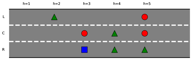
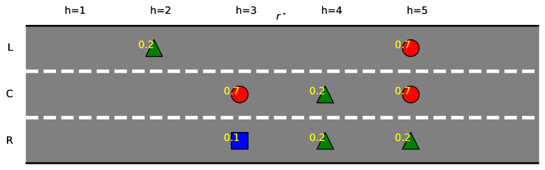
Figure 3: (Left) The target environment considered in the experiment. (Right) Representation of $r^{\star}$ for the target environment.

Finally, the occupancy measures $d^{p,\pi^{1}},d^{p,\pi^{2}}$ describing the application $g$ arise from the policies described in Section 5 and the transition model $p$ presented earlier, and are shown in Figure 4.

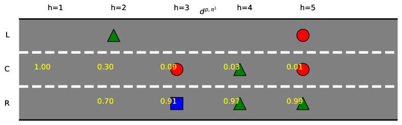
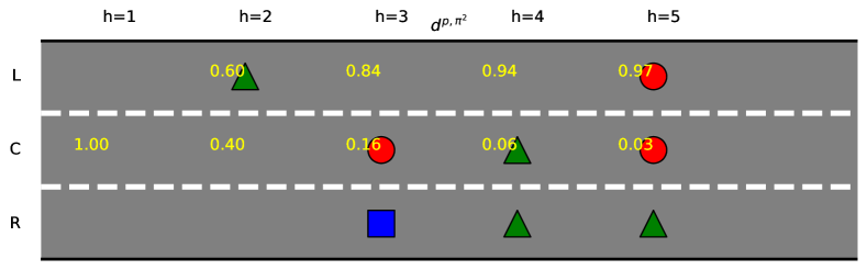
Figure 4: (Left) Plot of $d^{p,\pi^{1}}$. (Right) Plot of $d^{p,\pi^{2}}$.

C.5.2 Feedback $\mathcal{F}$

Trajectory comparisons.

We construct three trajectory comparison feedback. The first pair is in Figure 5, and we associated $t_{1}=0.3$ to it. The second pair of trajectories is in Figure 6, and we set $t_{2}=1$. Finally, the third pair is in Figure 7 and has $t_{3}=-0.5$.

Comparisons.

Concerning the comparisons feedback, we considered the new environment shown in Figure 8 on the left, keeping the same transition model $p$ described earlier but using the left $L$ lane as initial state. We compared the two occupancy measures in Figure 9 using $t_{1}=0$, and the two occupancy measures in Figure 10 using $t_{2}=0.5$.

Demonstrations.

For the demonstrations feedback, we adopted the map in Figure 8 on the right, preserving the transition model $p$, but using lane R as initial state. We considered only one feedback, whose policy has the occupancy measure in Figure 11, to which we associated $t_{1}=1$.

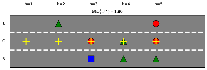
Figure 5: The trajectories compared in the first feedback. $\omega^{1}_{1}$ is on the left, and $\omega^{2}_{1}$ on the right.

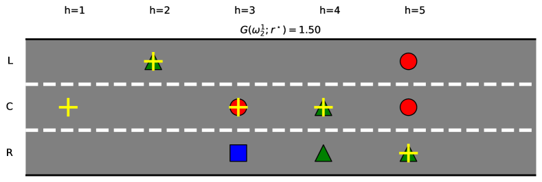
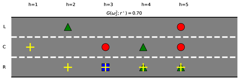
Figure 6: The trajectories compared in the second feedback. $\omega^{1}_{2}$ is on the left, and $\omega^{2}_{2}$ on the right.

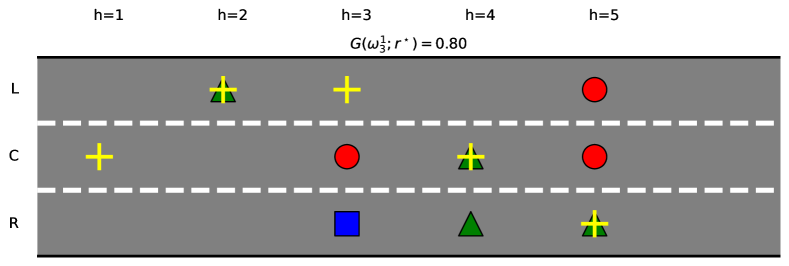
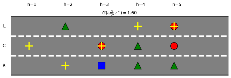
Figure 7: The trajectories compared in the third feedback. $\omega^{1}_{3}$ is on the left, and $\omega^{2}_{3}$ on the right.

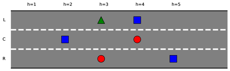
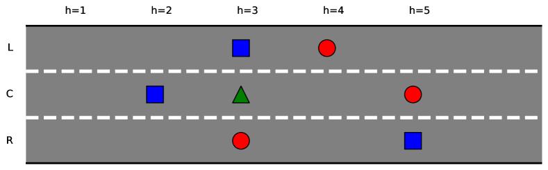
Figure 8: (Left) The new map considered for the comparisons feedback. (Right) The new map considered for the demonstrations feedback.

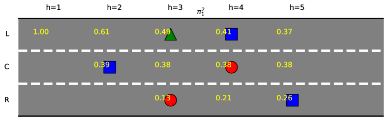
Figure 9: The occupancy measures compared in the first comparisons feedback. $\pi^{1}_{1}$ is on the left, and $\pi^{2}_{1}$ on the right.

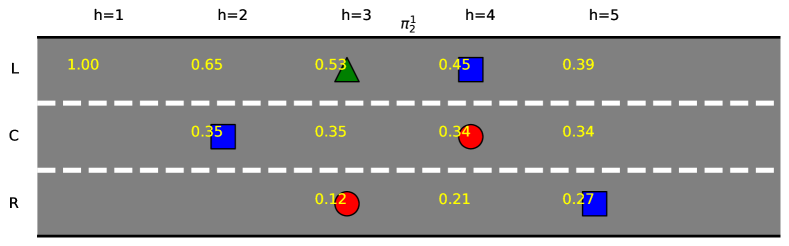
Figure 10: The occupancy measures compared in the second comparisons feedback. $\pi^{1}_{2}$ is on the left, and $\pi^{2}_{2}$ on the right.

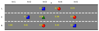
Figure 11: The occupancy measure of the expert’s policy for the demonstrations feedback.

C.5.3 Simulation

The execution of our algorithm generated the sequence of reward functions $\widehat{r}_{m,k}$ for finding $m$ and $r_{m}$ in Figure 12 on the left, while on the right we plotted the corresponding value of the objective function $\Delta J(\widehat{r}_{m,k})$.

The analogous plots for $M,r_{M}$ are in Figure 13.

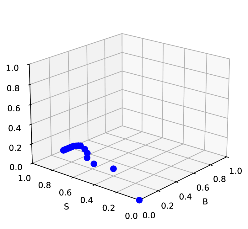
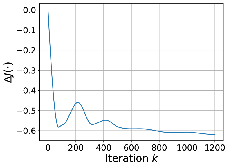
Figure 12: (Left) The sequence of rewards $\widehat{r}_{m,k}$ computed by our algorithm. (Right) The corresponding values of the objective function.

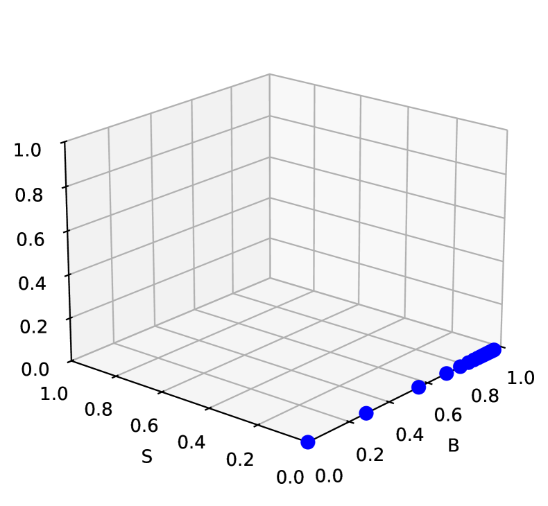
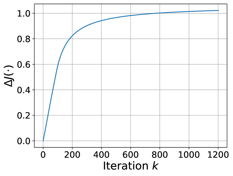
Figure 13: (Left) The sequence of rewards $\widehat{r}_{M,k}$ computed by our algorithm. (Right) The corresponding values of the objective function.

C.5.4 Values Computed “Exactly”

To understand if the values of $\widehat{r}_{M,K},\widehat{r}_{m,K},\widehat{r}$ extracted by our algorithm (see Figure 2) make sense, i.e., are close to the true values $r_{M},r_{m},r_{\mathcal{F},g}$, we have also computed them through an “exact” method, by computing a discretization of the feasible set and then taken the rewards that maximize/minimize the objective function (for approximating $r_{M},r_{m}$), and then averaged them. The results are in Figure 14. Clearly, these values are close to those in Figure 2, thus the results of our algorithms make sense.

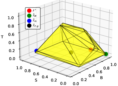
Figure 14: The rewards $r_{M},r_{m},r_{\mathcal{F},g}$ computed through a discretization of the feasible set.

Appendix D Active Learning

In the Active Learning setting (Lopes et al., 2009), in addition to a given set of feedback $\mathcal{F}$, we can choose to receive a new feedback $f^{\prime}$ from a set $\mathcal{F}^{\prime}=\{f_{i}^{\prime}\}_{i}$. Crucially, for any $f^{\prime}\in\mathcal{F}^{\prime}$, $f^{\prime}=(\mathcal{D},\mathbb{A})$, we consider the assumption $\mathbb{A}$ to be known, while the actual data $\mathcal{D}$ is revealed after our choice.

Example D.1.

We might choose between feedback $f_{1}=(\mathcal{D}_{1},\mathbb{A}^{\text{OPT}})$, consisting of demonstrations in environment $\mathcal{M}_{1}$ (i.e., $\mathcal{D}_{1}$) from an optimal expert (i.e., $\mathbb{A}^{\text{OPT}}$, see Example 3.5), or $f_{2}=(\mathcal{D}_{2},\mathbb{A}^{\text{MCE}})$, made of demonstrations in environment $\mathcal{M}_{2}$ (i.e., $\mathcal{D}_{2}$) from a maximal causal entropy expert (i.e., $\mathbb{A}^{\text{MCE}}$). After our choice, the expert demonstrates only one policy (i.e., either $\mathcal{D}_{1}$ or $\mathcal{D}_{2}$).

What is the “best” choice of feedback to receive without knowing its data $\mathcal{D}$? Thanks to our framework, and specifically to the notion of informativeness defined in Section 4, the immediate choice is the feedback that, whatever its true data, is the most “informative”.

Definition D.1 (Information gain).

We define the information gain $\text{IG}_{\mathcal{F},g}(f)$ of a feedback $f$ w.r.t. $g$ given $\mathcal{F}$ as:

In words, $\text{IG}_{\mathcal{F},g}(f)$ represents the reduction of (non)informativeness (worst-case error) of the ReL problem. Observe that $\text{IG}_{\mathcal{F},g}(f)\geq 0$, since $\overline{\mathcal{I}}_{\mathcal{F}\cup\{f\},g}\leq\overline{\mathcal{I}}_{\mathcal{F},g}$, i.e., the more feedback the less error.

Formally, the feedback that reduces the most the (non)informativeness is the feedback $f_{j}^{\prime}$ from set $\mathcal{F}^{\prime}=\{f_{i}^{\prime}\}_{i},f_{i}^{\prime}=(\mathcal{D}_{i},\mathbb{A}_{i})$, that maximizes the worst-case information gain w.r.t. the data $\mathcal{D}_{i}$:

Simply put, we select the feedback that, whatever the true data we will receive, we know that it will bring the larger reduction of informativeness, i.e., of error, for the ReL problem.

References

- Abbeel & Ng (2004) Abbeel, P. and Ng, A. Y. Apprenticeship learning via inverse reinforcement learning. In International Conference on Machine Learning 21 (ICML), 2004.
- Alimov & Tsar’kov (2019) Alimov, A. R. and Tsar’kov, I. G. Chebyshev centres, jung constants, and their applications. Russian Mathematical Surveys, 74, 2019.
- Amin & Singh (2016) Amin, K. and Singh, S. Towards resolving unidentifiability in inverse reinforcement learning, 2016.
- Arora & Doshi (2021) Arora, S. and Doshi, P. A survey of inverse reinforcement learning: Challenges, methods and progress. Artificial Intelligence, 297:103500, 2021.
- Boularias et al. (2011) Boularias, A., Kober, J., and Peters, J. Relative entropy inverse reinforcement learning. In International Conference on Artificial Intelligence and Statistics 14 (AISTATS 2011), pp. 182–189, 2011.
- Boyd & Vandenberghe (2004) Boyd, S. and Vandenberghe, L. Convex optimization. Cambridge university press, 2004.
- Boyd et al. (2022) Boyd, S., Duchi, J., Pilanci, M., and Vandenberghe, L. Subgradients, 2022. Notes for EE364b, Stanford University.
- Bubeck (2015) Bubeck, S. Convex optimization: Algorithms and complexity. Foundations and Trends in Machine Learning, 8(3–4):231–357, 2015.
- Cao et al. (2021) Cao, H., Cohen, S., and Szpruch, L. Identifiability in inverse reinforcement learning. In Advances in Neural Information Processing Systems 34 (NeurIPS), pp. 12362–12373, 2021.
- Christiano et al. (2017) Christiano, P. F., Leike, J., Brown, T., Martic, M., Legg, S., and Amodei, D. Deep reinforcement learning from human preferences. In Advances in Neural Information Processing Systems 30 (NeurIPS), 2017.
- Danzer et al. (1963) Danzer, L., Grünbaum, B., and Klee, V. Helly’s Theorem and Its Relatives. Proceedings of symposia in pure mathematics: Convexity. American Mathematical Society, 1963.
- Ding et al. (2020) Ding, D., Zhang, K., Basar, T., and Jovanovic, M. Natural policy gradient primal-dual method for constrained markov decision processes. In Advances in Neural Information Processing Systems 33 (NeurIPS), pp. 8378–8390, 2020.
- Fu et al. (2017) Fu, J., Luo, K., and Levine, S. Learning robust rewards with adversarial inverse reinforcement learning. In International Conference on Learning Representations 5 (ICLR), 2017.
- Haarnoja et al. (2017) Haarnoja, T., Tang, H., Abbeel, P., and Levine, S. Reinforcement learning with deep energy-based policies. In International Conference on Machine Learning 34 (ICML), volume 70, pp. 1352–1361, 2017.
- Hadfield-Menell et al. (2016) Hadfield-Menell, D., Russell, S. J., Abbeel, P., and Dragan, A. Cooperative inverse reinforcement learning. In Advances in Neural Information Processing Systems 29 (NeurIPS), 2016.
- Hadfield-Menell et al. (2017) Hadfield-Menell, D., Milli, S., Abbeel, P., Russell, S. J., and Dragan, A. Inverse reward design. In Advances in Neural Information Processing Systems 30 (NeurIPS), 2017.
- Ho & Ermon (2016) Ho, J. and Ermon, S. Generative adversarial imitation learning. In Advances in Neural Information Processing Systems 29 (NeurIPS), 2016.
- Ibarz et al. (2018) Ibarz, B., Leike, J., Pohlen, T., Irving, G., Legg, S., and Amodei, D. Reward learning from human preferences and demonstrations in atari. In Advances in Neural Information Processing Systems 32 (NeurIPS), pp. 8022–8034, 2018.
- Jeon et al. (2020) Jeon, H. J., Milli, S., and Dragan, A. Reward-rational (implicit) choice: A unifying formalism for reward learning. In Advances in Neural Information Processing Systems 33 (NeurIPS), pp. 4415–4426, 2020.
- Jung (1901) Jung, H. Ueber die kleinste kugel, die eine räumliche figur einschliesst. Journal für die reine und angewandte Mathematik, 123:241–257, 1901.
- Kaufmann et al. (2024) Kaufmann, T., Weng, P., Bengs, V., and Hüllermeier, E. A survey of reinforcement learning from human feedback, 2024.
- Kim et al. (2021) Kim, K., Garg, S., Shiragur, K., and Ermon, S. Reward identification in inverse reinforcement learning. In International Conference on Machine Learning 38 (ICML), pp. 5496–5505, 2021.
- Lacotte et al. (2019) Lacotte, J., Ghavamzadeh, M., Chow, Y., and Pavone, M. Risk-sensitive generative adversarial imitation learning. In International Conference on Artificial Intelligence and Statistics 22 (AISTATS), volume 89, pp. 2154–2163, 2019.
- Lazzati & Metelli (2024) Lazzati, F. and Metelli, A. M. Learning utilities from demonstrations in markov decision processes, 2024.
- Lazzati et al. (2024a) Lazzati, F., Mutti, M., and Metelli, A. M. How does inverse rl scale to large state spaces? a provably efficient approach, 2024a.
- Lazzati et al. (2024b) Lazzati, F., Mutti, M., and Metelli, A. M. Offline inverse rl: New solution concepts and provably efficient algorithms. In International Conference on Machine Learning 41 (ICML), 2024b.
- Lopes et al. (2009) Lopes, M., Melo, F., and Montesano, L. Active learning for reward estimation in inverse reinforcement learning. In Machine Learning and Knowledge Discovery in Databases (ECML PKDD), pp. 31–46, 2009.
- Malik et al. (2021) Malik, S., Anwar, U., Aghasi, A., and Ahmed, A. Inverse constrained reinforcement learning. In International Conference on Machine Learning 38 (ICML), volume 139, pp. 7390–7399, 2021.
- Menard et al. (2021) Menard, P., Domingues, O. D., Jonsson, A., Kaufmann, E., Leurent, E., and Valko, M. Fast active learning for pure exploration in reinforcement learning. In International Conference on Machine Learning 38 (ICML), volume 139, pp. 7599–7608, 2021.
- Metelli et al. (2021) Metelli, A. M., Ramponi, G., Concetti, A., and Restelli, M. Provably efficient learning of transferable rewards. In International Conference on Machine Learning 38 (ICML), volume 139, pp. 7665–7676, 2021.
- Metelli et al. (2023) Metelli, A. M., Lazzati, F., and Restelli, M. Towards theoretical understanding of inverse reinforcement learning. In International Conference on Machine Learning 40 (ICML), pp. 24555–24591, 2023.
- Nedić & Ozdaglar (2009) Nedić, A. and Ozdaglar, A. Subgradient methods for saddle-point problems. Journal of Optimization Theory and Applications, 142:205–228, 2009.
- Ng & Russell (2000) Ng, A. Y. and Russell, S. J. Algorithms for inverse reinforcement learning. In International Conference on Machine Learning 17 (ICML 2000), pp. 663–670, 2000.
- Ouyang et al. (2022) Ouyang, L., Wu, J., Jiang, X., Almeida, D., Wainwright, C., Mishkin, P., Zhang, C., Agarwal, S., Slama, K., Ray, A., Schulman, J., Hilton, J., Kelton, F., Miller, L., Simens, M., Askell, A., Welinder, P., Christiano, P. F., Leike, J., and Lowe, R. Training language models to follow instructions with human feedback. In Advances in Neural Information Processing Systems 35 (NeurIPS), pp. 27730–27744, 2022.
- Puterman (1994) Puterman, M. L. Markov Decision Processes: Discrete Stochastic Dynamic Programming. John Wiley & Sons, Inc., 1994.
- Ramachandran & Amir (2007) Ramachandran, D. and Amir, E. Bayesian inverse reinforcement learning. In International Joint Conference on Artifical Intelligence 20 (IJCAI), pp. 2586–2591, 2007.
- Ratliff et al. (2006) Ratliff, N. D., Bagnell, J. A., and Zinkevich, M. A. Maximum margin planning. In International Conference on Machine Learning 23 (ICML 2006), pp. 729–736, 2006.
- Russell (1998) Russell, S. Learning agents for uncertain environments (extended abstract). In Proceedings of the Eleventh Annual Conference on Computational Learning Theory 11 (COLT), pp. 101–103, 1998.
- Scott (1991) Scott, P. An extension of jung’s theorem. The Quarterly Journal of Mathematics, 42:209–212, 1991.
- Skalse & Abate (2024) Skalse, J. and Abate, A. Quantifying the sensitivity of inverse reinforcement learning to misspecification. In International Conference on Learning Representations 12 (ICLR), 2024.
- Skalse et al. (2023a) Skalse, J., Farnik, L., Motwani, S. R., Jenner, E., Gleave, A., and Abate, A. Starc: A general framework for quantifying differences between reward functions. In International Conference on Learning Representations 11 (ICLR), 2023a.
- Skalse et al. (2023b) Skalse, J. M. V., Farrugia-Roberts, M., Russell, S., Abate, A., and Gleave, A. Invariance in policy optimisation and partial identifiability in reward learning. In International Conference on Machine Learning 40 (ICML), volume 202, pp. 32033–32058, 2023b.
- Syed & Schapire (2007) Syed, U. and Schapire, R. E. A game-theoretic approach to apprenticeship learning. In Advances in Neural Information Processing System 20 (NeurIPS), 2007.
- Wirth et al. (2017) Wirth, C., Akrour, R., Neumann, G., and Fürnkranz, J. A survey of preference-based reinforcement learning methods. Journal of Machine Learning Research, 18:4945–4990, 2017.
- Wulfmeier et al. (2016) Wulfmeier, M., Ondruska, P., and Posner, I. Maximum entropy deep inverse reinforcement learning, 2016.
- Zhao et al. (2024) Zhao, L., Wang, M., and Bai, Y. Is inverse reinforcement learning harder than standard reinforcement learning? In International Conference on Machine Learning 41 (ICML), 2024.
- Zhu et al. (2023) Zhu, B., Jordan, M., and Jiao, J. Principled reinforcement learning with human feedback from pairwise or k-wise comparisons. In International Conference on Machine Learning 40 (ICML), volume 202, pp. 43037–43067, 2023.
- Ziebart (2010) Ziebart, B. D. Modeling purposeful adaptive behavior with the principle of maximum causal entropy, 2010.
- Ziebart et al. (2008) Ziebart, B. D., Maas, A., Bagnell, J. A., and Dey, A. K. Maximum entropy inverse reinforcement learning. In AAAI Conference on Artificial Intelligence 23 (AAAI), volume 3, pp. 1433–1438, 2008.