Analysis of a Shear beam model with suspenders
in thermoelasticity of type III

Abstract.

We conduct an analysis of a one-dimensional linear problem that describes the vibrations of a connected suspension bridge. In this model, the single-span roadbed is represented as a thermoelastic Shear beam without rotary inertia. We incorporate thermal dissipation into the transverse displacement equation, following Green and Naghdi’s theory. Our work demonstrates the existence of a global solution by employing classical Faedo–Galerkin approximations and three a priori estimates. Furthermore, we establish exponential stability through the application of the energy method. For numerical study, we propose a spatial discretization using finite elements and a temporal discretization through an implicit Euler scheme. In doing so, we prove discrete stability properties and a priori error estimates for the discrete problem. To provide a practical dimension to our theoretical findings, we present a set of numerical simulations.

1. Introduction

A cable-suspended beam is a structural design comprising a beam that is upheld by one or more cables. These cables have the dual role of bearing the beam’s weight and preserving its shape to enhance stability and provide additional support. Cable-suspended beams find applications in a range of engineering contexts, including cable-stayed bridges and suspension bridges [31].

In this paper, we address a thermomechanical problem associated with a cable-suspended beam structure, exemplified by the suspension bridge. The key characteristic of this structure is that the roadbed’s sectional dimensions are significantly smaller than its length (span of the bridge). Suspension bridges with large span lengths exhibit higher flexibility in comparison to alternative bridge structures. This increased flexibility renders them vulnerable to various dynamic loads, including wind, earthquakes, and the movement of vehicles. The distinctive structural features of suspension bridges elevate the significance of understanding their dynamic response to oscillations, presenting a crucial engineering challenge. Therefore, we model the roadbed as an extensible thermoelastic Shear-type beam. The primary suspension cable is represented as an elastic string, and it is linked to the roadbed through a distributed network of elastic springs. Our model aligns with the configuration of a Shear-suspended-beam system within thermoelasticity of type III, as described in the following:

$$\begin{cases}\rho u_{tt}-\alpha u_{xx}-\lambda\left(\varphi-u\right)+\mu u_{t}=0,&\text{in}\;(0,L)\times(0,\infty),\\ \rho_{1}\varphi_{tt}-K\left(\varphi_{x}+\psi\right)_{x}+\lambda\left(\varphi-u\right)+\gamma\varphi_{t}+\beta\theta_{x}=0,&\text{in}\;(0,L)\times(0,\infty),\\ -b\psi_{xx}+K\left(\varphi_{x}+\psi\right)=0,&\text{in}\;(0,L)\times(0,\infty),\\ \rho_{3}\theta_{tt}-\delta\theta_{xx}+\beta\varphi_{xtt}-\kappa\theta_{xxt}=0,&\text{in}\;(0,L)\times(0,\infty),\\ u(0,t)=u(L,t)=\varphi(0,t)=\varphi(L,t)=0,&t\geqslant 0,\\ \psi(0,t)=\psi(L,t)=\theta(0,t)=\theta(L,t)=0,&t\geqslant 0,\\ u(x,0)=u_{0}(x),\;u_{t}(x,0)=u_{1}(x),\;\varphi(x,0)=\varphi_{0}(x),\;\varphi_{t}(x,0)=\varphi_{1}(x),&x\in(0,L),\\ \psi(x,0)=\psi_{0}(x),\;\theta(x,0)=\theta_{0}(x),\;\theta_{t}(x,0)=\theta_{1}(x),&x\in(0,L).\end{cases}$$ (1.1)

Here, the symbol $t$ represents the time variable, while $x$ denotes the distance along the centerline of the beam in its equilibrium configuration. Both $L$ and the beam length coincide with the cable length. Within this framework, we use the following notations: $u$ represents the vertical displacement of the vibrating spring in the primary cable; $\varphi$ signifies the transverse displacement or vertical deflection of the beam’s cross-section; $\psi$ denotes the angle of rotation of a cross-section; while $\theta$ is employed to represent the thermal moment of the beam. We consider the suspender cables (ties) as linear elastic springs with a shared stiffness parameter $\lambda>0$, and the constant $\alpha>0$ defines the elastic modulus of the string that connects the cable to the deck. The constants $\rho$, $\mu$, $\rho_{1}$, $\rho_{3}$, $K$, $\gamma$, $\kappa$, $\delta$, and $\beta\neq 0$, employed in the problem formulation, are positive. The initial data, denoted as $(u_{0},u_{1},\varphi_{0},\varphi_{1},\psi_{0},\theta_{0},\theta_{1})$, belong to an appropriate functional space.

For many years, there has been substantial research interest in the dynamic behavior and nonlinear vibrations of suspension bridges [2, 3, 4, 19]. Suspension bridges are complex structures with distinctive dynamic characteristics, and they can display nonlinear responses to various external forces and loads. This nonlinearity may stem from factors such as large-amplitude vibrations, material properties, and environmental conditions. The appearance of string-beam systems that model a nonlinear coupling of a beam (the roadbed) and main cable (the string) were born out of the pioneering works of Lazer and McKenna [26, 27]. Elimination of nonlinear coupling terms in the equations of motion governing vertical and torsional vibrations of suspension bridges is achieved by linearization, as indicated in reference [1]. Previous approaches have often employed models where the roadbed was based on the Euler-Bernoulli beam theory [10, 11, 12, 13]. The Timoshenko beam theory has also demonstrated superior performance in anticipating the vibrational response of a beam compared to a model grounded in the classical Euler-Bernoulli beam theory [24].

It is worth noting that the Euler–Bernoulli beam theory and the Timoshenko beam theory are two different approaches to model the behavior of beams. The Euler–Bernoulli beam theory assumes that the beam is slender and that the cross-section remains plane and perpendicular to the longitudinal axis of the beam during deformation. This theory is suitable for modeling long and slender beams that are subjected to bending loads. On the other hand, the Timoshenko beam theory takes into account the effects of shear deformation and rotational bending, which makes this theory more accurate for analyzing short and thick beams. The Timoshenko equations [34] improved the Euler–Bernoulli and the Rayleigh beam models and such equations are given by

$$\begin{cases}\rho_{1}\varphi_{tt}-K\left(\varphi_{x}+\psi\right)_{x}=0,\\ \rho_{2}\psi_{tt}-b\psi_{xx}+K\left(\varphi_{x}+\psi\right)=0.\\ \end{cases}$$

The Euler–Bernoulli beam theory used to represent the single-span roadbed has neglected the effects of shear deformation and rotary inertia. These effects can be taken into account by using more accurate models, such as the Timoshenko beam theory to have a deeper range of applicability and to be physically more realistic [7, 25]. Bochicchio et al. examined a linear problem that characterizes the vibrations of a coupled suspension bridge [9]. In their analysis, the single-span roadbed is represented as an extensible thermoelastic beam following the Timoshenko model, with heat governed by Fourier’s law. They demonstrated the exponential decay property by employing the established semi-group theory and the energy method. Additionally, they conducted several numerical experiments to further support their findings. Mukiawa et al. utilized the same methods to establish the existence and uniqueness of a weak global solution and to demonstrate exponential stability in a thermal-Timoshenko-beam system [30]. This system incorporated suspenders and Kelvin–Voigt damping and was founded on the principles of thermoelasticity, as described by Cattaneo’s law.

The Timoshenko beam formulation is generally considered for determining the dynamic response of beams at higher frequencies (higher wave numbers), where there exist two frequency values. As a result, when there are two wave speeds $\sqrt{K/\rho_{1}}$ and $\sqrt{b/\rho_{2}}$, one of the wave speeds has an infinite speed (blow-up) for lower wave numbers. To overcome this physical drawback, simplified beam models have been introduced, as the truncated version for dissipative Timoshenko type system [5], and the Shear beam model given by

$$\begin{cases}\rho_{1}\varphi_{tt}-K\left(\varphi_{x}+\psi\right)_{x}=0,\\ -b\psi_{xx}+K\left(\varphi_{x}+\psi\right)=0,\\ \end{cases}$$

which has only one finite wave speed $\sqrt{K/\rho_{1}}$ for all wave numbers. Almeida Júnior et al. [6] and Ramos et al. [33] were pioneers in investigating the well-posedness and stability characteristics of the Shear beam model. This model constitutes an improvement over the Euler–Bernoulli beam model by adding the shear distortion effect but without rotary inertia. Consequently, one can analyze long-span bridges, unlike the Timoshenko beam theory, which is better suited for modeling beams with relatively short spans. This is precisely our focus here – the examination of the Shear model (1.1) with suspenders and thermal dissipation, introduced by thermoelasticity of Type III.

The second major aspect of problem (1.1) under investigation in this paper concerns what is referred to as thermoelasticity of type III. In classical theory of thermoelasticity, heat conduction is typically described using Fourier’s law for heat flux. This theory has the un-physical property that a sudden temperature change at some point will be felt instantly everywhere (that is, the heat propagation has an infinite speed). However, experiments have shown that the speed of the thermal wave propagation in some dielectric crystals at low temperatures is limited. This phenomenon in dielectric crystals is called the second sound. In the modern theory of thermal propagation, there are several ways to overcome this physical paradox. The most known is the one that proposes replacing Fourier’s law of heat flux with Cattaneo’s law [15], in order to obtain a heat conduction equation of hyperbolic type that describes the wave nature of heat propagation at low temperatures. At the turn of the century, Green and Naghdi introduced three other theories (known as thermoelasticity Type I, Type II, and Type III), based on the equality of entropy rather than the usual entropy inequality [21, 22, 23]. In each theory, the heat flux is determined by different appropriate assumptions. These three theories give a comprehensive and logical explanation that embodies the transmission of a thermal pulse and modifies the occurrence of the infinite unphysical speed of heat propagation induced by the classical theory of heat conduction. When the theory of type I is linearized, it aligns with the classical system of thermoelasticity. The systems arising in thermoelasticity of type III exhibit dissipative characteristics, while those in type II do not sustain energy dissipation. It is a limiting case of thermoelasticity type III [16, 17, 29, 32, 35].

Numerically, the finite element method has been utilized in various research studies related to control systems [8, 20].

The paper’s structure is outlined as follows. In Section 2, we provide some preliminary information. To demonstrate the global existence and uniqueness of solutions, in Section 3 we revisit the Faedo–Galerkin method, along with three estimates, previously discussed in references such as [18, 28]. In Section 4, we employ the energy method to construct several Lyapunov functionals, establishing the property of exponential decay. In Section 5, we propose a finite element discretization approach to solve the problem at hand. We obtain discrete stability results and a priori error estimates. Finally, in Section 6, we present some numerical simulations using MATLAB.

Throughout the paper, the symbols $C$ and $C_{i}$ are used to represent various positive constants.

2. Preliminaries

In the following, $(\cdot,\cdot)$ represents the scalar product of $L_{2}(0,L)$, and $\lVert\cdot\rVert$ denotes the norm $\lVert\cdot\rVert_{L_{2}(0,L)}$. In order to exhibit the dissipative nature of system (1.1), we introduce the new variable

$$w(x,t)=\int_{0}^{t}\theta(x,s)ds+\eta(x),$$ (2.1)

where $\eta(x)$ solves

$$\begin{cases}\delta\Delta\eta=\rho_{3}\theta_{1}-\kappa\Delta\theta_{0}+\beta\nabla\cdot\varphi_{1},\\ \eta(0)=\eta(1)=0.\end{cases}$$ (2.2)

Performing an integration of ${\text{(\ref{main:system*})}}_{\text{4}}$ with respect to $t$ and taking into account (2.1), we get

$$\begin{split}\int_{0}^{t}\left(\rho_{3}\theta_{tt}-\delta\theta_{xx}+\beta\varphi_{xtt}-\kappa\theta_{xxt}\right)ds&=0\\ \rho_{3}w_{tt}-\rho_{3}\theta_{1}-\left(\delta w_{xx}-\delta\Delta\eta\right)+\beta\varphi_{xt}-\beta\nabla\cdot\varphi_{1}-\kappa w_{xxt}+\kappa\Delta\theta_{0}&=0.\end{split}$$

Then (2.2) gives

$$\rho_{3}w_{tt}-\delta w_{xx}+\beta\varphi_{xt}-\kappa w_{xxt}=0,$$

and problem (1.1) takes the form

$$\begin{cases}\rho u_{tt}-\alpha u_{xx}-\lambda\left(\varphi-u\right)+\mu u_{t}=0,&\text{in}\;(0,L)\times(0,\infty),\\ \rho_{1}\varphi_{tt}-K\left(\varphi_{x}+\psi\right)_{x}+\lambda\left(\varphi-u\right)+\gamma\varphi_{t}+\beta w_{xt}=0,&\text{in}\;(0,L)\times(0,\infty),\\ -b\psi_{xx}+K\left(\varphi_{x}+\psi\right)=0,&\text{in}\;(0,L)\times(0,\infty),\\ \rho_{3}w_{tt}-\delta w_{xx}+\beta\varphi_{xt}-\kappa w_{xxt}=0,&\text{in}\;(0,L)\times(0,\infty),\\ u(0,t)=u(L,t)=\varphi(0,t)=\varphi(L,t)=0,&t\geqslant 0,\\ \psi(0,t)=\psi(L,t)=w(0,t)=w(L,t)=0,&t\geqslant 0,\\ u(x,0)=u_{0}(x),\;u_{t}(x,0)=u_{1}(x),\;\varphi(x,0)=\varphi_{0}(x),\;\varphi_{t}(x,0)=\varphi_{1}(x),&x\in(0,L),\\ \psi(x,0)=\psi_{0}(x),\;w(x,0)=w_{0}(x),\;w_{t}(x,0)=w_{1}(x),&x\in(0,L).\end{cases}$$ (2.3)

Lemma 2.1.

Let $(u,\varphi,\psi,w)$ be the solution of (2.3). Then the energy functional $E$, defined by

$$E(t)=\dfrac{1}{2}\int_{0}^{L}\left(\rho u_{t}^{2}+\alpha u_{x}^{2}+\lambda(\varphi-u)^{2}+\rho_{1}\varphi_{t}^{2}+K{(\varphi_{x}+\psi)}^{2}+b\psi_{x}^{2}+\rho_{3}w_{t}^{2}+\delta w_{x}^{2}\right)dx,$$ (2.4)

satisfies

$$\dfrac{dE(t)}{dt}=-\mu\int_{0}^{L}u_{t}^{2}dx-\gamma\int_{0}^{L}\varphi_{t}^{2}dx-\kappa\int_{0}^{L}w_{xt}^{2}dx\leqslant 0,\;\forall\;t\geqslant 0.$$ (2.5)

Proof.

We multiply the equations in (2.3) by $u_{t}$, $\varphi_{t}$, $\psi_{t}$, $w_{t}$, respectively, and integrate by parts to get

$$\dfrac{1}{2}\dfrac{d}{dt}\left(\rho\int_{0}^{L}u_{t}^{2}dx\right)+\dfrac{1}{2}\dfrac{d}{dt}\left(\alpha\int_{0}^{L}u_{x}^{2}dx\right)+\dfrac{1}{2}\dfrac{d}{dt}\left(\lambda\int_{0}^{L}u^{2}dx\right)-\lambda\int_{0}^{L}\varphi u_{t}dx+\mu\int_{0}^{L}u_{t}^{2}dx=0,$$ (2.6)

$$\begin{split}\dfrac{1}{2}\dfrac{d}{dt}\left(\rho_{1}\int_{0}^{L}\varphi_{t}^{2}dx\right)&+\dfrac{1}{2}\dfrac{d}{dt}\left(K\int_{0}^{L}\varphi_{x}^{2}dx\right)+K\int_{0}^{L}\psi\varphi_{xt}dx+\dfrac{1}{2}\dfrac{d}{dt}\left(\lambda\int_{0}^{L}\varphi^{2}dx\right)\\ &-\lambda\int_{0}^{L}u\varphi_{t}dx+\gamma\int_{0}^{L}\varphi_{t}^{2}dx+\beta\int_{0}^{L}w_{xt}\varphi_{t}dx=0,\end{split}$$ (2.7)

$$\dfrac{1}{2}\dfrac{d}{dt}\left(b\int_{0}^{L}\psi^{2}_{x}dx\right)+\dfrac{1}{2}\dfrac{d}{dt}\left(K\int_{0}^{L}\psi^{2}dx\right)+K\int_{0}^{L}\varphi_{x}\psi_{t}dx=0,$$ (2.8)

$$\dfrac{1}{2}\dfrac{d}{dt}\left(\rho_{3}\int_{0}^{L}w_{t}^{2}dx\right)+\kappa\int_{0}^{L}w_{xt}^{2}dx+\beta\int_{0}^{L}\varphi_{xt}w_{t}dx+\dfrac{1}{2}\dfrac{d}{dt}\left(\delta\int_{0}^{L}w_{x}^{2}dx\right)=0.$$ (2.9)

Adding (2.6)–(2.9), we obtain (2.5). These calculations are done for any regular solution. Nonetheless, the same result holds valid for weak solutions by using density arguments. ∎

Theorem 2.2 (Aubin–Lions–Simon theorem, see p. 102 of [14]).

Let $B_{0}\subset B_{1}\subset B_{2}$ be three Banach spaces. We assume that the embedding of $B_{1}$ in $B_{2}$ is continuous and that the embedding of $B_{0}$ in $B_{1}$ is compact. Let $p$ and $r$ such that $1\leqslant p,r\leqslant+\infty$. For $T>0$, we define

$$W_{p,r}=\left\{\chi\in L^{p}(]0,T[,B_{0}),\dfrac{d\chi}{dt}\in L^{r}(]0,T[,B_{2})\right\}.$$

1. If $p<+\infty$, the embedding of $W_{p,r}$ in $L^{p}(]0,T[,B_{1})$ is compact.

2. If $p=+\infty$ and if $r>1$, the embedding of $W_{p,r}$ in $C([0,T],B_{1})$ is compact.

3. Global well‑posedness

In this section we prove the existence and uniqueness of regular and weak solutions for system (2.3) by using the Faedo–Galerkin method.

Theorem 3.1.

1. If the initial data $u_{0},\varphi_{0},\psi_{0},w_{0}$ $\in H^{1}_{0}(0,L)$ and $u_{1},\varphi_{1},w_{1}\in L^{2}(0,L)$, then problem (2.3) has a unique weak solution satisfying

   $$u,\varphi,w\in C([0,T],H^{1}_{0}(0,L))\cap C^{1}([0,T],L^{2}(0,L)),\;\psi\in C([0,T],H^{1}_{0}(0,L)).$$ (3.1)

2. If the initial data $u_{0},\varphi_{0},\psi_{0},w_{0}$ $\in H^{2}(0,L)\cap H^{1}_{0}(0,L)$ and $u_{1},\varphi_{1},w_{1}\in H^{1}_{0}(0,L)$, then the weak solution (3.1) has higher regularity:

   $$\begin{split}u,\varphi,w\in C([0,T],H^{2}(0&,L)\cap H^{1}_{0}(0,L))\cap C^{1}([0,T],H^{1}_{0}(0,L))\cap C^{2}([0,T],L^{2}(0,L)),\\ &\psi\in C([0,T],H^{2}(0,L)\cap H^{1}_{0}(0,L)).\end{split}$$ (3.2)

Proof.

We prove the result in six steps.

Step 1: approximated problem. Suppose that $u_{0}$, $\varphi_{0}$, $\psi_{0}$, $w_{0}$ $\in H^{2}(0,L)\cap H^{1}_{0}(0,L)$, $u_{1}$, $\varphi_{1}$, $w_{1}$ $\in H^{1}_{0}(0,L)$. Let $\left\{v_{i}\right\}_{i\in\mathbb{N}}$ be a smooth orthonormal basis of $L^{2}(0,L)$, which is also orthogonal in $H^{2}(0,L)\cap H^{1}_{0}(0,L)$, given by the eigenfunctions of $-\Delta v=\varsigma v$ with boundary condition $v(0)=v(L)=0$, such that

$$-\Delta v_{i}=\varsigma_{i}v_{i}.$$ (3.3)

Here $\varsigma_{i}$ is the eigenvalue corresponding to $v_{i}$. For any $m\in\mathbb{N}$, denote by $V_{m}$ the finite-dimensional subspace

$$\begin{split}V_{m}&=span\left\{v_{1},v_{2},\ldots,v_{m}\right\}\subset H^{2}(0,L)\cap H^{1}_{0}(0,L).\end{split}$$

To construct the Galerkin approximation $(u^{m},\varphi^{m},\psi^{m},w^{m})$ of the solution, let us denote

$$u^{m}(t)=\sum_{i=1}^{m}g_{im}(t)v_{i}(x),\;\varphi^{m}(t)=\sum_{i=1}^{m}\hat{g}_{im}(t)v_{i}(x),$$

$$\psi^{m}(t)=\sum_{i=1}^{m}f_{im}(t)v_{i}(x),\;w^{m}(t)=\sum_{i=1}^{m}\hat{f}_{im}(t)v_{i}(x),$$

where functions $g_{im}$, $\hat{g}_{im}$, $f_{im}$, $\hat{f}_{im}\in C^{2}[0,T]$ are given by the solution of the approximated system

$$\begin{cases}\rho(u_{tt}^{m}(t),v_{i})+\alpha(u_{x}^{m}(t),v_{ix})-\lambda(\varphi^{m}(t)-u^{m}(t),v_{i})+\mu(u^{m}_{t}\left(t\right),v_{i})=0,\\ \begin{split}\rho_{1}(\varphi_{tt}^{m}(t),v_{i})+K(\varphi_{x}^{m}(t)&+\psi^{m}(t),v_{ix})+\lambda(\varphi^{m}(t)-u^{m}(t),v_{i})\\ &+\gamma(\varphi^{m}_{t}\left(t\right),v_{i})+\beta(w_{xt}^{m}(t),v_{i})=0,\end{split}\\ b(\psi^{m}_{x}\left(t\right),v_{ix})+K\left(\varphi^{m}_{x}(t)+\psi^{m}(t),v_{i}\right)=0,\\ \rho_{3}(w^{m}_{tt}(t),v_{i})+\delta(w^{m}_{x}(t),v_{ix})+\beta(\varphi_{xt}^{m}(t),v_{i})+\kappa(w^{m}_{xt}(t),v_{ix})=0,\end{cases}$$ (3.4)

with the initial conditions

$$u^{m}(0)=u^{m}_{0}=\sum_{i=1}^{m}(u_{0},v_{i})v_{i}\xrightarrow{m\rightarrow\infty}u_{0}\;\;\text{in}\;H^{2}(0,L)\cap H^{1}_{0}(0,L),$$ (3.5)

$$\varphi^{m}(0)=\varphi^{m}_{0}=\sum_{i=1}^{m}(\varphi_{0},v_{i})v_{i}\xrightarrow{m\rightarrow\infty}\varphi_{0}\;\;\text{in}\;H^{2}(0,L)\cap H^{1}_{0}(0,L),$$ (3.6)

$$\psi^{m}(0)=\psi^{m}_{0}=\sum_{i=1}^{m}(\psi_{0},v_{i})v_{i}\xrightarrow{m\rightarrow\infty}\psi_{0}\;\;\text{in}\;H^{2}(0,L)\cap H^{1}_{0}(0,L),$$ (3.7)

$$w^{m}(0)=w^{m}_{0}=\sum_{i=1}^{m}(w_{0},v_{i})v_{i}\xrightarrow{m\rightarrow\infty}w_{0}\;\;\text{in}\;H^{2}(0,L)\cap H^{1}_{0}(0,L),$$ (3.8)

$$u^{m}_{t}(0)=u^{m}_{1}=\sum_{i=1}^{m}(u_{1},v_{i})v_{i}\xrightarrow{m\rightarrow\infty}u_{1}\;\;\text{in}\;H^{1}_{0}(0,L),$$ (3.9)

$$\varphi^{m}_{t}(0)=\varphi^{m}_{1}=\sum_{i=1}^{m}(\varphi_{1},v_{i})v_{i}\xrightarrow{m\rightarrow\infty}\varphi_{1}\;\;\text{in}\;H^{1}_{0}(0,L),$$ (3.10)

$$w^{m}_{t}(0)=w^{m}_{1}=\sum_{i=1}^{m}(w_{1},v_{i})v_{i}\xrightarrow{m\rightarrow\infty}w_{1}\;\;\text{in}\;H^{1}_{0}(0,L).$$ (3.11)

From the theory of ODEs, system (3.4)–(3.11) has a unique local solution $(u^{m}(t),\varphi^{m}(t),\psi^{m}(t),w^{m}(t))$ defined on $[0,T_{m})$ with $0<T_{m}<T$. Our next step is to show that the local solution is extended to $[0,T]$ for any given $T>0$.

Step 2: first a priori estimate. Multiplying ${\text{(\ref{appro:problem})}}_{\text{1}}$, ${\text{(\ref{appro:problem})}}_{\text{2}}$, ${\text{(\ref{appro:problem})}}_{\text{3}}$ and ${\text{(\ref{appro:problem})}}_{\text{4}}$ by $g^{\prime}_{im}$, $\hat{g}^{\prime}_{im}$, $f^{\prime}_{im}$ and $\hat{f}^{\prime}_{im}$, respectively, summing up over $i$ from $1$ to $m$, taking the sum of the resulting equations and using integration by parts, we obtain that

$$\begin{split}&\dfrac{d}{dt}\left(\dfrac{\rho}{2}{\rVert u^{m}_{t}(t)\lVert}^{2}+\dfrac{\alpha}{2}{\rVert u^{m}_{x}(t)\lVert}^{2}+\dfrac{\lambda}{2}{\rVert\varphi^{m}(t)-u^{m}(t)\lVert}^{2}+\dfrac{\rho_{1}}{2}{\rVert\varphi^{m}_{t}(t)\lVert}^{2}\right)\\ &+\dfrac{d}{dt}\left(\dfrac{K}{2}{\rVert\varphi^{m}_{x}(t)+\psi^{m}(t)\lVert}^{2}+\dfrac{b}{2}{\lVert\psi^{m}_{x}(t)\rVert}^{2}+\dfrac{\rho_{3}}{2}{\lVert w_{t}^{m}(t)\rVert}^{2}+\dfrac{\delta}{2}{\lVert w_{x}^{m}(t)\rVert}^{2}\right)\\ &+\mu{\lVert u_{t}^{m}(t)\rVert}^{2}+\gamma{\lVert\varphi_{t}^{m}(t)\rVert}^{2}+\kappa{\lVert w_{xt}^{m}(t)\rVert}^{2}=0.\end{split}$$ (3.12)

Integrating (3.12) over $(0,t)$, we find

$$\mathcal{E}^{m}_{1}(t)+\mu\int_{0}^{t}{\lVert u_{t}^{m}(s)\rVert}^{2}ds+\gamma\int_{0}^{t}{\lVert\varphi_{t}^{m}(s)\rVert}^{2}ds+\kappa\int_{0}^{t}{\lVert w_{xt}^{m}(s)\rVert}^{2}ds=\mathcal{E}^{m}_{1}(0),$$ (3.13)

where

$$\begin{split}\mathcal{E}^{m}_{1}(t)=&\dfrac{1}{2}\left(\rho{\rVert u^{m}_{t}(t)\lVert}^{2}+\alpha{\rVert u^{m}_{x}(t)\lVert}^{2}+\lambda{\rVert\varphi^{m}(t)-u^{m}(t)\lVert}^{2}+\rho_{1}{\rVert\varphi^{m}_{t}(t)\lVert}^{2}\right)\\ &+\dfrac{1}{2}\left(K{\rVert\varphi_{x}^{m}(t)+\psi^{m}(t)\lVert}^{2}+b{\rVert\psi^{m}_{x}(t)\lVert}^{2}+\rho_{3}{\lVert w_{t}^{m}(t)\rVert}^{2}+\delta{\lVert w_{x}^{m}(t)\rVert}^{2}\right).\end{split}$$ (3.14)

From (3.13), we deduce that there exists $C$, independent of $m$, such that

$$\mathcal{E}^{m}_{1}(t)\leqslant\mathcal{E}^{m}_{1}(0)\leqslant C,\;t\geqslant 0.$$ (3.15)

Consequently, we have

$$\begin{split}&{\rVert u^{m}_{t}(t)\lVert}^{2}+{\rVert u^{m}_{x}(t)\lVert}^{2}+{\rVert\varphi^{m}(t)-u^{m}(t)\lVert}^{2}+{\rVert\varphi^{m}_{t}(t)\lVert}^{2}\\ &+{\rVert\varphi_{x}^{m}(t)+\psi^{m}(t)\lVert}^{2}+{\rVert\psi^{m}_{x}(t)\lVert}^{2}+{\lVert w_{t}^{m}(t)\rVert}^{2}+{\lVert w_{x}^{m}(t)\rVert}^{2}\leqslant C.\end{split}$$ (3.16)

The estimate (3.16) implies that the solution $(u^{m},\varphi^{m},\psi^{m},w^{m})$ exists globally in $[0,\infty)$ and, for any $m\in\mathbb{N}$,

$$u^{m},\;\varphi^{m},\;\psi^{m},\;w^{m}\;\;\text{are bounded in }\;L^{\infty}(0,T;H^{1}_{0}(0,L)),$$ (3.17)

$$u^{m}_{t},\;\varphi^{m}_{t},\;w^{m}_{t}\;\;\text{are bounded in }\;L^{\infty}(0,T;L^{2}(0,L)).$$ (3.18)

Step 3: second a priori estimate. Taking the derivative of the approximate equations in (3.4) with respect to $t$, we get

$$\begin{cases}\rho(u_{ttt}^{m}(t),v_{i})+\alpha(u^{m}_{xt}(t),v_{ix})-\lambda(\varphi_{t}^{m}(t)-u^{m}_{t}(t),v_{i})+\mu(u^{m}_{tt}\left(t\right),v_{i})=0,\\ \begin{split}\rho_{1}(\varphi_{ttt}^{m}(t),v_{i})+K(\varphi_{xt}^{m}(t)&+\psi^{m}_{t}(t),v_{ix})+\lambda(\varphi_{t}^{m}(t)-u^{m}_{t}(t),v_{i})\\ &+\gamma(\varphi^{m}_{tt}\left(t\right),v_{i})+\beta(w^{m}_{xtt},v_{i})=0,\end{split}\\ b(\psi^{m}_{xt}\left(t\right),v_{ix})+K\left(\varphi^{m}_{xt}(t)+\psi^{m}_{t}(t),v_{i}\right)=0,\\ \rho_{3}(w_{ttt}^{m}(t),v_{i})+\delta(w_{xt}^{m}(t),v_{ix})+\beta(\varphi_{xtt}^{m}(t),v_{i})+\kappa(w^{m}_{xtt},v_{ix})=0.\end{cases}$$ (3.19)

Multiplying ${\text{(\ref{appro:problem2})}}_{\text{1}}$, ${\text{(\ref{appro:problem2})}}_{\text{2}}$, ${\text{(\ref{appro:problem2})}}_{\text{3}}$ and ${\text{(\ref{appro:problem2})}}_{\text{4}}$ by $g^{\prime\prime}_{im}$, $\hat{g}^{\prime\prime}_{im}$, $f^{\prime\prime}_{im}$ and $\hat{f}^{\prime\prime}_{im}$, respectively, and summing up over $i$ from $1$ to $m$, it follows that

$$\dfrac{1}{2}\dfrac{d}{dt}\left(\rho{\rVert u^{m}_{tt}(t)\lVert}^{2}\right)+\dfrac{1}{2}\dfrac{d}{dt}\left(\alpha{\rVert u^{m}_{tx}(t)\lVert}^{2}\right)-\lambda\int_{0}^{L}(\varphi^{m}_{t}(t)-u^{m}_{t}(t))u^{m}_{tt}(t)dx+\mu{\rVert u^{m}_{tt}(t)\lVert}^{2}=0,$$ (3.20)

$$\begin{split}\dfrac{1}{2}\dfrac{d}{dt}&\left(\rho_{1}{\rVert\varphi^{m}_{tt}(t)\lVert}^{2}\right)+K\int_{0}^{L}(\varphi^{m}_{xt}(t)+\psi^{m}_{t}(t))\varphi^{m}_{xtt}(t)dx+\gamma{\rVert\varphi^{m}_{tt}(t)\lVert}^{2}\\ &+\lambda\int_{0}^{L}(\varphi^{m}_{t}(t)-u^{m}_{t}(t))\varphi^{m}_{tt}(t)dx+\beta\int_{0}^{L}w^{m}_{xtt}(t)\varphi^{m}_{tt}(t)dx=0,\end{split}$$ (3.21)

$$\begin{split}\dfrac{1}{2}\dfrac{d}{dt}\left(b{\lVert\psi^{m}_{xt}(t)\rVert}^{2}\right)+K\int_{0}^{L}(\varphi^{m}_{xt}(t)+\psi^{m}_{t}(t))\psi^{m}_{tt}(t)dx=0,\end{split}$$ (3.22)

$$\dfrac{1}{2}\dfrac{d}{dt}\left(\rho_{3}{\rVert w^{m}_{tt}(t)\lVert}^{2}\right)+\dfrac{1}{2}\dfrac{d}{dt}\left(\delta{\rVert w^{m}_{xt}(t)\lVert}^{2}\right)+\beta\int_{0}^{L}\varphi^{m}_{xt}(t)w_{tt}^{m}(t)dx+\kappa{\rVert w^{m}_{xtt}(t)\lVert}^{2}=0.$$ (3.23)

Adding up (3.20)–(3.23) and using integration by parts, we obtain that

$$\begin{split}&\dfrac{d}{dt}\left(\dfrac{\rho}{2}{\rVert u^{m}_{tt}(t)\lVert}^{2}+\dfrac{\alpha}{2}{\rVert u^{m}_{xt}(t)\lVert}^{2}+\dfrac{\lambda}{2}{\rVert\varphi_{t}^{m}(t)-u_{t}^{m}(t)\lVert}^{2}+\dfrac{\rho_{1}}{2}{\rVert\varphi^{m}_{tt}(t)\lVert}^{2}\right)\\ &+\dfrac{d}{dt}\left(\dfrac{K}{2}{\rVert\varphi^{m}_{xt}(t)+\psi_{t}^{m}(t)\lVert}^{2}+\dfrac{b}{2}{\lVert\psi^{m}_{xt}(t)\rVert}^{2}+\dfrac{\rho_{3}}{2}{\lVert w_{tt}^{m}(t)\rVert}^{2}+\dfrac{\delta}{2}{\lVert w_{xt}^{m}(t)\rVert}^{2}\right)\\ &+\mu{\lVert u_{tt}^{m}(t)\rVert}^{2}+\gamma{\lVert\varphi_{tt}^{m}(t)\rVert}^{2}+\kappa{\lVert w_{xtt}^{m}(t)\rVert}^{2}=0.\end{split}$$ (3.24)

Now, integrating (3.24) over $(0,t)$, yields

$$\mathcal{E}^{m}_{2}(t)+\mu\int_{0}^{t}{\lVert u_{tt}^{m}(s)\rVert}^{2}ds+\gamma\int_{0}^{t}{\lVert\varphi_{tt}^{m}(s)\rVert}^{2}ds+\kappa\int_{0}^{t}{\lVert w_{xtt}^{m}(s)\rVert}^{2}ds=\mathcal{E}^{m}_{2}(0),$$ (3.25)

where

$$\begin{split}\mathcal{E}^{m}_{2}(t)=&\dfrac{1}{2}\left(\rho{\rVert u^{m}_{tt}(t)\lVert}^{2}+\alpha{\rVert u^{m}_{xt}(t)\lVert}^{2}+\lambda{\rVert\varphi_{t}^{m}(t)-u_{t}^{m}(t)\lVert}^{2}+\rho_{1}{\rVert\varphi^{m}_{tt}(t)\lVert}^{2}\right)\\ &+\dfrac{1}{2}\left(K{\rVert\varphi_{xt}^{m}(t)+\psi_{t}^{m}(t)\lVert}^{2}+b{\rVert\psi^{m}_{xt}(t)\lVert}^{2}+\rho_{3}{\lVert w_{tt}^{m}(t)\rVert}^{2}+\delta{\lVert w_{xt}^{m}(t)\rVert}^{2}\right).\end{split}$$ (3.26)

Thus, there exists $C$ independent of $m$ such that

$$\mathcal{E}^{m}_{2}(t)\leqslant\mathcal{E}^{m}_{2}(0)\leqslant C,\;t\geqslant 0,$$ (3.27)

accordingly

$$\begin{split}&{\rVert u^{m}_{tt}(t)\lVert}^{2}+{\rVert u^{m}_{xt}(t)\lVert}^{2}+{\rVert\varphi_{t}^{m}(t)-u_{t}^{m}(t)\lVert}^{2}+{\rVert\varphi^{m}_{tt}(t)\lVert}^{2}\\ &+{\rVert\varphi_{xt}^{m}(t)+\psi_{t}^{m}(t)\lVert}^{2}+{\rVert\psi^{m}_{xt}(t)\lVert}^{2}+{\lVert w_{tt}^{m}(t)\rVert}^{2}+{\lVert w_{xt}^{m}(t)\rVert}^{2}\leqslant C,\end{split}$$ (3.28)

and, for any $m\in\mathbb{N}$, we have

$$u_{t}^{m},\;\varphi^{m}_{t},\;\psi^{m}_{t},\;w^{m}_{t}\;\;\text{bounded in }\;L^{\infty}(0,T;H^{1}_{0}(0,L)),$$ (3.29)

$$u^{m}_{tt},\;\varphi^{m}_{tt},\;w^{m}_{tt}\;\;\text{bounded in }\;L^{\infty}(0,T;L^{2}(0,L)).$$ (3.30)

Step 4: third a priori estimate. Replacing $v_{i}$ by $-v_{ixx}$ in (3.4) and multiplying the resulting equations by $g^{\prime}_{im}$, $\hat{g}^{\prime}_{im}$, $f^{\prime}_{im}$ and $\hat{f}^{\prime}_{im}$, respectively, summing over $i$ from $1$ to $m$ and using integration by parts, we obtain that

$$\dfrac{1}{2}\dfrac{d}{dt}\left(\rho{\rVert u^{m}_{xt}(t)\lVert}^{2}\right)+\dfrac{1}{2}\dfrac{d}{dt}\left(\alpha{\rVert u^{m}_{xx}(t)\lVert}^{2}\right)-\lambda\int_{0}^{L}(\varphi^{m}_{x}(t)-u^{m}_{x}(t))u^{m}_{xt}(t)dx+\mu{\rVert u^{m}_{xt}(t)\lVert}^{2}=0,$$ (3.31)

$$\begin{split}\dfrac{1}{2}\dfrac{d}{dt}&\left(\rho_{1}{\rVert\varphi^{m}_{xt}(t)\lVert}^{2}\right)+K\int_{0}^{L}(\varphi^{m}_{xx}(t)+\psi^{m}_{x}(t))\varphi^{m}_{xxt}(t)dx+\gamma{\rVert\varphi^{m}_{xt}(t)\lVert}^{2}\\ &+\lambda\int_{0}^{L}(\varphi^{m}_{x}(t)-u^{m}_{x}(t))\varphi^{m}_{xt}(t)dx-\beta\int_{0}^{L}w^{m}_{xt}(t)\varphi^{m}_{xxt}(t)dx=0,\end{split}$$ (3.32)

$$\begin{split}\dfrac{1}{2}\dfrac{d}{dt}\left(b{\lVert\psi^{m}_{xx}(t)\rVert}^{2}\right)-K\int_{0}^{L}(\varphi^{m}_{x}(t)+\psi^{m}(t))\psi^{m}_{xxt}(t)dx=0,\end{split}$$ (3.33)

$$\dfrac{1}{2}\dfrac{d}{dt}\left(\rho_{3}{\rVert w^{m}_{xt}(t)\lVert}^{2}\right)+\dfrac{1}{2}\dfrac{d}{dt}\left(\delta{\rVert w^{m}_{xx}(t)\lVert}^{2}\right)+\beta\int_{0}^{L}\varphi^{m}_{xxt}(t)w_{xt}^{m}(t)dx+\kappa{\rVert w^{m}_{xxt}(t)\lVert}^{2}=0.$$ (3.34)

Taking the sum of (3.31)–(3.34) and integrating over $(0,t)$, one has

$$\begin{split}\mathcal{E}^{m}_{3}(t)+\mu\int_{0}^{t}{\lVert u_{xt}^{m}(s)\rVert}^{2}ds+\gamma\int_{0}^{t}{\lVert\varphi_{xt}^{m}(s)\rVert}^{2}ds+\kappa\int_{0}^{t}{\lVert w_{xxt}^{m}(s)\rVert}^{2}ds=\mathcal{E}^{m}_{3}(0),\end{split}$$ (3.35)

where

$$\begin{split}\mathcal{E}^{m}_{3}(t)=&\dfrac{1}{2}\left(\rho{\rVert u^{m}_{xt}(t)\lVert}^{2}+\alpha{\rVert u^{m}_{xx}(t)\lVert}^{2}+\lambda{\rVert\varphi_{x}^{m}(t)-u_{x}^{m}(t)\lVert}^{2}+\rho_{1}{\rVert\varphi^{m}_{xt}(t)\lVert}^{2}\right)\\ &+\dfrac{1}{2}\left(K{\rVert\varphi_{xx}^{m}(t)+\psi_{x}^{m}(t)\lVert}^{2}+b{\rVert\psi^{m}_{xx}(t)\lVert}^{2}+\rho_{3}{\lVert w_{xt}^{m}(t)\rVert}^{2}+\delta{\lVert w_{xx}^{m}(t)\rVert}^{2}\right).\end{split}$$ (3.36)

Then, there exists $C$, independent of $m$, such that

$$\mathcal{E}^{m}_{3}(t)\leqslant\mathcal{E}^{m}_{3}(0)\leqslant C,\;t\geqslant 0,$$

which entails that

$$\begin{split}&{\rVert u^{m}_{xt}(t)\lVert}^{2}+{\rVert u^{m}_{xx}(t)\lVert}^{2}+{\rVert\varphi_{x}^{m}(t)-u_{x}^{m}(t)\lVert}^{2}+{\rVert\varphi^{m}_{xt}(t)\lVert}^{2}\\ &+{\rVert\varphi_{xx}^{m}(t)+\psi_{x}^{m}(t)\lVert}^{2}+{\rVert\psi^{m}_{xx}(t)\lVert}^{2}+{\lVert w_{xt}^{m}(t)\rVert}^{2}+{\lVert w_{xx}^{m}(t)\rVert}^{2}\leqslant C.\end{split}$$ (3.37)

For all $m\in\mathbb{N}$, (3.37) implies that

$$u^{m},\;\varphi^{m},\;\psi^{m},\;w^{m}\;\;\text{are bounded in }\;L^{\infty}(0,T;H^{2}(0,L)\cap H^{1}_{0}(0,L)).$$ (3.38)

Step 5: passage to the limit. Thanks to (3.29), (3.30) and (3.38), and passing to a subsequence, if necessary, we have

$$\begin{cases}u^{m}\rightharpoonup^{\ast}u\;\;\text{ in }\;L^{\infty}(0,T;H^{2}(0,L)\cap H^{1}_{0}(0,L)),\\ u^{m}_{t}\rightharpoonup^{\ast}u_{t}\;\;\text{ in }\;L^{\infty}(0,T;H^{1}_{0}(0,L)),\\ u^{m}_{tt}\rightharpoonup^{\ast}u_{tt}\;\;\text{ in }\;L^{\infty}(0,T;L^{2}(0,L)),\end{cases}$$ (3.39)

$$\begin{cases}\varphi^{m}\rightharpoonup^{\ast}\varphi\;\;\text{ in }\;L^{\infty}(0,T;H^{2}(0,L)\cap H^{1}_{0}(0,L)),\\ \varphi^{m}_{t}\rightharpoonup^{\ast}\varphi_{t}\;\;\text{ in }\;L^{\infty}(0,T;H^{1}_{0}(0,L)),\\ \varphi^{m}_{tt}\rightharpoonup^{\ast}\varphi_{tt}\;\;\text{ in }\;L^{\infty}(0,T;L^{2}(0,L)),\end{cases}$$ (3.40)

$$\begin{cases}\psi^{m}\rightharpoonup^{\ast}\psi\;\;\text{ in }\;L^{\infty}(0,T;H^{2}(0,L)\cap H^{1}_{0}(0,L)),\\ \psi^{m}_{t}\rightharpoonup^{\ast}\psi_{t}\;\;\text{ in }\;L^{\infty}(0,T;H^{1}_{0}(0,L)),\end{cases}$$ (3.41)

$$\begin{cases}w^{m}\rightharpoonup^{\ast}w\;\;\text{ in }\;L^{\infty}(0,T;H^{2}(0,L)\cap H^{1}_{0}(0,L)),\\ w^{m}_{t}\rightharpoonup^{\ast}w_{t}\;\;\text{ in }\;L^{\infty}(0,T;H^{1}_{0}(0,L)),\\ w^{m}_{tt}\rightharpoonup^{\ast}w_{tt}\;\;\text{ in }\;L^{\infty}(0,T;L^{2}(0,L)).\end{cases}$$ (3.42)

From the above limits, we conclude that $(u,u_{t},\varphi,\varphi_{t},\psi,w,w_{t})$ is a strong weak solution with higher regularity, satisfying

$$u,\varphi,\psi,w\in L^{\infty}(0,T;H^{2}(0,L)\cap H^{1}_{0}(0,L)),\quad u_{t},\varphi_{t},w_{t}\in L^{\infty}(0,T;H^{1}_{0}(0,L)).$$

The embedding $H^{2}(0,L)\cap H^{1}_{0}(0,L)$ in $H^{1}_{0}(0,L)$ is compact. Note that if we let $B_{1}=B_{2}=H^{1}_{0}(0,L)$ and $B_{0}=H^{2}(0,L)\cap H^{1}_{0}(0,L)$ in Aubin–Lions–Simon Theorem 2.2, then we get that the embedding of $W_{\infty,\infty}$ in $C(]0,T[,H^{1}_{0}(0,L))$ is compact, where

$$W_{\infty,\infty}=\left\{u^{m}:\;u^{m}\in L^{\infty}(]0,T[,H^{2}(0,L)\cap H^{1}_{0}(0,L)),u^{m}_{t}\in L^{\infty}(]0,T[,H^{1}_{0}(0,L))\right\}.$$

Now, from (3.39), we deduce that $u^{m}$ is bounded in $W_{\infty,\infty}$ and, therefore, we can extract a subsequence $(u^{\nu})$ of $(u^{m})$ such that

$$u^{\nu}\longrightarrow u\;\;\text{ in }\;C([0,T],H^{1}_{0}(0,L)).$$ (3.43)

Similarly, we obtain

$$\psi^{\nu}\longrightarrow\psi\;\;\text{ in }\;C([0,T],H^{1}_{0}(0,L)),$$

$$\varphi^{\nu}\longrightarrow\varphi\;\;\text{ in }\;C([0,T],H^{1}_{0}(0,L)),$$

$$w^{\nu}\longrightarrow w\;\;\text{ in }\;C([0,T],H^{1}_{0}(0,L)).$$

Since the embedding $H^{1}_{0}(0,L)\hookrightarrow L^{2}(0,L)$ is compact, going back again to the compactness Theorem 2.2 with $B_{0}=H^{1}_{0}(0,L)$, $B_{1}=B_{2}=L^{2}(0,L)$ and $\chi=u^{m}_{t}$, gives

$$u^{\nu}_{t}\longrightarrow u_{t}\;\;\text{ in }\;C([0,T],L^{2}(0,L)),$$ (3.44)

where here $(u^{\nu}_{t})$ is a subsequence of $(u^{m}_{t})$. Similarly, we find

$$\varphi^{\nu}_{t}\longrightarrow\varphi_{t}\;\;\text{ in }\;C([0,T],L^{2}(0,L)),$$

$$w^{\nu}_{t}\longrightarrow w_{t}\;\;\text{ in }\;C([0,T],L^{2}(0,L)).$$

On the other hand, note that

$$-u^{\nu}_{xx}=\varsigma u^{\nu}\;\text{ and }\;C([0,T],H^{1}_{0}(0,L))\subset C([0,T],L^{2}(0,L)).$$

Then, from (3.43), we infer that

$$u^{\nu}\longrightarrow u\;\;\text{ in }\;C([0,T],H^{2}(0,L)\cap H^{1}_{0}(0,L)).$$

Now, making use of (3.43) and (3.44), respectively, with the dominated convergence theorem (differentiating under the integral sign), gives that

$$\lVert u^{\nu}_{t}-u_{t}\rVert_{C([0,T],H^{1}_{0}(0,L))}\xrightarrow{\nu\rightarrow\infty}0,$$

$$\lVert u^{\nu}_{tt}-u_{tt}\rVert_{C([0,T],L^{2}(0,L))}\xrightarrow{\nu\rightarrow\infty}0,$$

which implies that

$$u^{\nu}_{t}\longrightarrow u_{t}\;\;\text{ in }\;C([0,T],H^{1}_{0}(0,L)),$$

$$u^{\nu}_{tt}\longrightarrow u_{tt}\;\;\text{ in }\;C([0,T],L^{2}(0,L)).$$

The same arguments are used to determine the limits of $\varphi^{\nu},\varphi^{\nu}_{t},\varphi^{\nu}_{tt},\psi^{\nu},w^{\nu},w^{\nu}_{t}$ and $w^{\nu}_{tt}$. With these limits, we can pass to the limit of the terms of the approximate equations in (3.4) to get a strong weak solution to problem (2.3).

Step 6: continuous dependence and uniqueness. Let $(u,u_{t},\varphi,\varphi_{t},\psi,w,w_{t})$ and $(\tilde{u},\tilde{u}_{t},\tilde{\varphi},\tilde{\varphi}_{t},\tilde{\psi},\tilde{w},\tilde{w}_{t})$ be strong solutions of problem (2.3). Then,

$$(U,U_{t},\Lambda,\Lambda_{t},X,\Theta,\Theta_{t})=(u-\tilde{u},u_{t}-\tilde{u}_{t},\varphi-\tilde{\varphi},\varphi_{t}-\tilde{\varphi}_{t},\psi-\tilde{\psi},w-\tilde{w},w_{t}-\tilde{w}_{t})$$

satisfies

$$\rho U_{tt}\left(x,t\right)-\alpha U_{xx}\left(x,t\right)-\lambda(\Lambda-U)\left(x,t\right)+\mu U_{t}\left(x,t\right)=0,$$ (3.45)

$$\rho_{1}\Lambda_{tt}\left(x,t\right)-K\left(\Lambda_{x}+X\right)_{x}\left(x,t\right)+\lambda(\Lambda-U)\left(x,t\right)+\gamma\Lambda_{t}(x,t)+\beta\Theta_{xt}(x,t)=0,$$ (3.46)

$$-bX_{xx}\left(x,t\right)+K\left(\Lambda_{x}+X\right)\left(x,t\right)=0,$$ (3.47)

$$\rho_{3}\Theta_{tt}(x,t)-\delta\Theta_{xx}(x,t)+\beta\Lambda_{xt}(x,t)-\kappa\Theta_{xxt}(x,t)=0,$$ (3.48)

with the initial data

$$\begin{split}U(0)&=u(0)-\tilde{u}(0),\\ U_{t}(0)&=u_{t}(0)-\tilde{u}_{t}(0),\\ \Lambda(0)&=\varphi(0)-\tilde{\varphi}(0),\\ \Lambda_{t}(0)&=\varphi_{t}(0)-\tilde{\varphi}_{t}(0),\\ X(0)&=\psi(0)-\tilde{\psi}(0),\\ \Theta(0)&=w(0)-\tilde{w}(0),\\ \Theta_{t}(0)&=w_{t}(0)-\tilde{w}_{t}(0).\end{split}$$

Repeating exactly the same arguments used to obtain the estimate (2.5), we get

$$\dfrac{d\tilde{E}(t)}{dt}=-\mu{\rVert U_{t}\lVert}^{2}-\gamma{\rVert\Lambda_{t}\lVert}^{2}-\kappa{\rVert\Theta_{xt}\lVert}^{2}.$$ (3.49)

Integrating (3.49) over $(0,t)$, we conclude that

$$\tilde{E}(t)\leqslant C_{T}\tilde{E}(0),\;t\in[0,T],$$

for some constant $C_{T}>0$, which proves the continuous dependence of the solutions on the initial data. In particular, the stronger weak solution is unique.

To demonstrate the existence of weak solutions, let us consider the initial data $u_{0},\varphi_{0},\psi_{0},w_{0}$ $\in H^{1}_{0}(0,L)$ and $u_{1},\varphi_{1},w_{1}\in L^{2}(0,L)$ in the approximate problem (3.4). Then, by density, we have

$$u^{m}_{0},\varphi^{m}_{0},\psi^{m}_{0},w^{m}_{0}\rightarrow u_{0},\varphi_{0},\psi_{0},w_{0}\;\;\text{in}\;H^{1}_{0}(0,L),\;u^{m}_{1},\varphi^{m}_{1},w^{m}_{1}\rightarrow u_{1},\varphi_{1},w_{1}\;\;\text{in}\;L^{2}(0,L).$$ (3.50)

Repeating the same steps used in the first estimate, following the same procedure already used in the uniqueness of strong solutions for $(U^{m},U_{t}^{m},\Lambda^{m},\Lambda_{t}^{m},X^{m},\Theta^{m},\Theta_{t}^{m})=(u^{m}-\tilde{u}^{m},u_{t}^{m}-\tilde{u}_{t}^{m},\varphi^{m}-\tilde{\varphi}^{m},\varphi_{t}^{m}-\tilde{\varphi}_{t}^{m},\psi^{m}-\tilde{\psi}^{m},w^{m}-\tilde{w}^{m},w_{t}^{m}-\tilde{w}_{t}^{m})$ and taking into account the convergences (3.50), we deduce that there exists $u$, $\varphi$, $\psi$, and $w$ such that

$$u^{m}\longrightarrow u\;\;\text{ in }\;C([0,T],H^{1}_{0}(0,L)),$$

$$\psi^{m}\longrightarrow\psi\;\;\text{ in }\;C([0,T],H^{1}_{0}(0,L)),$$

$$\varphi^{m}\longrightarrow\varphi\;\;\text{ in }\;C([0,T],H^{1}_{0}(0,L)),$$

$$w^{m}\longrightarrow w\;\;\text{ in }\;C([0,T],H^{1}_{0}(0,L)),$$

$$u^{m}_{t}\longrightarrow u_{t}\;\;\text{ in }\;C([0,T],L^{2}(0,L)),$$

$$\varphi^{m}_{t}\longrightarrow\varphi_{t}\;\;\text{ in }\;C([0,T],L^{2}(0,L)),$$

$$w^{m}_{t}\longrightarrow w_{t}\;\;\text{ in }\;C([0,T],L^{2}(0,L)).$$

The uniqueness is obtained making use of the well-known regularization procedure, as presented in [28, Chapter 3, Section 8.2.2]. ∎

4. Exponential stability

The main result of this section is to prove the following stability theorem for regular solution, since the same occurs for weak solution using standard density arguments.

Theorem 4.1.

With the regularity stated in Theorem 3.1, the energy $E(t)$ decays exponentially as time approaches infinity, that is, there exists two positive constants, $\sigma_{0}$ and $\sigma_{1}$, such that

$$E(t)\leqslant\sigma_{0}e^{-\sigma_{1}t}\quad\forall t\geqslant 0.$$ (4.1)

We begin by proving some important lemmas that will be essential to prove Theorem 4.1.

Lemma 4.2.

The functional

$$I_{1}(t)=\int_{0}^{L}\left(\rho u_{t}u+\dfrac{\mu}{2}u^{2}\right)dx+\int_{0}^{L}\left(\rho_{1}\varphi_{t}\varphi+\dfrac{\gamma}{2}\varphi^{2}\right)dx$$

satisfies

$$\begin{split}\dfrac{dI_{1}(t)}{dt}\leqslant&-\alpha\int_{0}^{L}u_{x}^{2}dx-\lambda\int_{0}^{L}(\varphi-u)^{2}dx-\dfrac{K}{2}\int_{0}^{L}(\varphi_{x}+\psi)^{2}dx\\ &-\dfrac{b}{2}\int_{0}^{L}\psi^{2}_{x}dx+\rho\int_{0}^{L}u_{t}^{2}dx+\rho_{1}\int_{0}^{L}\varphi_{t}^{2}dx+C_{1}\int_{0}^{L}w^{2}_{xt}dx.\end{split}$$ (4.2)

Proof.

Multiplying ${\text{(\ref{main:system})}}_{\text{1}}$ by $u$, using the fact that $u_{tt}u=\dfrac{\partial}{\partial t}(u_{t}u)-u_{t}^{2}$ and integrating by parts, we get that

$$\dfrac{d}{dt}\int_{0}^{L}\left(\rho u_{t}u+\dfrac{\mu}{2}u^{2}\right)dx-\rho\int_{0}^{L}u_{t}^{2}dx+\alpha\int_{0}^{L}u_{x}^{2}dx-\lambda\int_{0}^{L}(\varphi-u)udx=0.$$ (4.3)

Similarly, multiplying ${\text{(\ref{main:system})}}_{\text{2}}$ by $\varphi$, using the fact that $\varphi_{tt}\varphi=\dfrac{\partial}{\partial t}(\varphi_{t}\varphi)-\varphi_{t}^{2}$ and integrating by parts, one obtains

$$\begin{split}\dfrac{d}{dt}\int_{0}^{L}\left(\rho_{1}\varphi_{t}\varphi+\dfrac{\gamma}{2}\varphi^{2}\right)dx&-\rho_{1}\int_{0}^{L}\varphi_{t}^{2}dx+K\int_{0}^{L}(\varphi_{x}+\psi)\varphi_{x}dx\\ &+\lambda\int_{0}^{L}\left(\varphi-u\right)\varphi dx+\beta\int_{0}^{L}w_{xt}\varphi dx=0.\end{split}$$ (4.4)

Now, multiplying ${\text{(\ref{main:system})}}_{\text{3}}$ by $\psi$, it results that

$$b\int_{0}^{L}\psi_{x}^{2}dx+K\int_{0}^{L}(\varphi_{x}+\psi)\psi dx=0.$$ (4.5)

Adding (4.3)–(4.5), we arrive at

$$\begin{split}\dfrac{dI_{1}(t)}{dt}=&\rho\int_{0}^{L}u_{t}^{2}dx-\alpha\int_{0}^{L}u_{x}^{2}dx-\lambda\int_{0}^{L}(\varphi-u)^{2}dx+\rho_{1}\int_{0}^{L}\varphi_{t}^{2}dx\\ &-K\int_{0}^{L}(\varphi_{x}+\psi)^{2}dx-b\int_{0}^{L}\psi_{x}^{2}dx+\beta\int_{0}^{L}w_{t}\varphi_{x}dx.\end{split}$$ (4.6)

The fact that $\varphi_{x}=(\varphi_{x}+\psi)-\psi$ leads to

$$\beta\int_{0}^{L}w_{t}\varphi_{x}dx=\beta\int_{0}^{L}w_{t}(\varphi_{x}+\psi)dx-\beta\int_{0}^{L}w_{t}\psi dx$$ (4.7)

and Young’s and Poincaré’s inequalities yield that

$$\beta\int_{0}^{L}w_{t}(\varphi_{x}+\psi)dx\leqslant\dfrac{K}{2}\int_{0}^{L}(\varphi_{x}+\psi)^{2}dx+\dfrac{\beta^{2}c_{p}}{2K}\int_{0}^{L}w_{xt}^{2}dx,$$ (4.8)

$$-\beta\int_{0}^{L}w_{t}\psi dx\leqslant\dfrac{b}{2}\int_{0}^{L}\psi_{x}^{2}dx+\dfrac{\beta^{2}c^{2}_{p}}{2b}\int_{0}^{L}w_{xt}^{2}dx,$$ (4.9)

where $c_{p}$ is a Poincaré’s constant. We obtain (4.2) by plugging (4.8) and (4.9) into (4.6). ∎

Lemma 4.3.

The functional

$$I_{2}(t)=\rho_{3}\int_{0}^{L}w_{t}wdx+\dfrac{\kappa}{2}\int_{0}^{L}w_{x}^{2}dx+\beta\int_{0}^{L}\varphi_{x}wdx$$

satisfies

$$\dfrac{dI_{2}(t)}{dt}\leqslant-\delta\int_{0}^{L}w_{x}^{2}dx+\dfrac{b}{4}\int_{0}^{L}\psi_{x}^{2}dx+\dfrac{K}{4}\int_{0}^{L}(\varphi_{x}+\psi)^{2}dx+C_{2}\int_{0}^{L}w_{xt}^{2}dx.$$ (4.10)

Proof.

Differentiating $I_{2}$, using ${\text{(\ref{main:system})}}_{\text{4}}$, integration by parts and recalling the boundary conditions, we get that

$$\dfrac{dI_{2}(t)}{dt}=\rho_{3}\int_{0}^{L}w_{t}^{2}dx-\delta\int_{0}^{L}w_{x}^{2}dx+\beta\int_{0}^{L}w_{t}\varphi_{x}dx.$$ (4.11)

It follows by (4.7) and Young’s and Poincaré’s inequalities that

$$\beta\int_{0}^{L}w_{t}(\varphi_{x}+\psi)dx\leqslant\dfrac{K}{4}\int_{0}^{L}(\varphi_{x}+\psi)^{2}dx+\dfrac{\beta^{2}c_{p}}{K}\int_{0}^{L}w_{xt}^{2}dx$$ (4.12)

and

$$-\beta\int_{0}^{L}w_{t}\psi dx\leqslant\dfrac{b}{4}\int_{0}^{L}\psi_{x}^{2}dx+\dfrac{\beta^{2}c^{2}_{p}}{b}\int_{0}^{L}w_{xt}^{2}dx.$$ (4.13)

Applying Poincaré’s inequality leads to

$$\rho_{3}\int_{0}^{L}w_{t}^{2}dx\leqslant\rho_{3}c_{p}\int_{0}^{L}w_{xt}^{2}dx.$$ (4.14)

By substituting (4.12), (4.13) and (4.14) into (4.11), we obtain that (4.10) holds. ∎

Let us introduce now the Lyapunov functional

$$L(t)=NE(t)+I_{1}(t)+I_{2}(t),$$ (4.15)

where $N$ is a positive constant to be fixed later.

Lemma 4.4.

Let $(u,\varphi,\psi,w)$ be a solution of (2.3). Then there exist two positive constants, $\xi_{1}$ and $\xi_{2}$, such that the functional energy $E$ is equivalent to functional $L$:

$$\xi_{1}E(t)\leqslant L(t)\leqslant\xi_{2}E(t).$$ (4.16)

Proof.

We know that

$$\begin{split}\left|L(t)-NE(t)\right|\leqslant&\rho\int_{0}^{L}\left|u_{t}u\right|dx+\dfrac{\mu}{2}\int_{0}^{L}u^{2}dx+\rho_{1}\int_{0}^{L}\left|\varphi_{t}\varphi\right|dx+\dfrac{\gamma}{2}\int_{0}^{L}\varphi^{2}dx\\ &+\rho_{3}\int_{0}^{L}\left|w_{t}w\right|dx+\dfrac{\kappa}{2}\int_{0}^{L}w_{x}^{2}dx+\left|\beta\right|\int_{0}^{L}\left|\varphi_{x}w\right|dx.\end{split}$$

By using $\varphi_{x}=(\varphi_{x}+\psi)-\psi$, $u=-(\varphi-u)+\varphi$, and Young’s and Poincarés inequalities, we obtain, for some $\xi>0$, that

$$\left|L(t)-NE(t)\right|\leqslant\xi E(t),$$

which yields

$$(N-\xi)E(t)\leqslant L(t)\leqslant(N+\xi)E(t).$$

The estimate (4.16) follows by choosing $N$ accordingly. ∎

We are now in conditions to prove Theorem 4.1.

Proof.

(of Theorem 4.1) Taking the time derivative of $L(t)$, using Lemmas 4.2 and 4.3 and the energy dissipation law (2.5), it follows from (4.15) that

$$\begin{split}\dfrac{dL(t)}{dt}\leqslant&-\alpha\int_{0}^{L}u_{x}^{2}dx-\lambda\int_{0}^{L}(\varphi-u)^{2}dx\\ &-\dfrac{K}{4}\int_{0}^{L}(\varphi_{x}+\psi)^{2}dx-\dfrac{b}{4}\int_{0}^{L}\psi_{x}^{2}dx-\delta\int_{0}^{1}w_{x}^{2}dx\\ &-\left[N\mu-\rho\right]\int_{0}^{L}u_{t}^{2}dx-\left[N\gamma-\rho_{1}\right]\int_{0}^{L}\varphi_{t}^{2}dx\\ &-\left[N\kappa-C_{1}-C_{2}\right]\int_{0}^{1}w_{xt}^{2}dx.\end{split}$$

Next, we choose $N$ large enough so that (4.16) remains valid and

$$\begin{cases}N\mu-\rho>0,\\ N\gamma-\rho_{1}>0,\\ N\kappa-C_{1}-C_{2}>0.\end{cases}$$

Thus, for some $\zeta_{1}>0$, we have

$$\dfrac{dL(t)}{dt}\leqslant-\zeta_{1}\int_{0}^{L}[u_{t}^{2}+u_{x}^{2}+(\varphi-u)^{2}+\varphi_{t}^{2}+(\varphi_{x}+\psi)^{2}+\psi_{x}^{2}+w_{xt}^{2}+w_{x}^{2}]\;dx.$$

On account of (2.4), we can write that

$$\dfrac{dL(t)}{dt}\leqslant-\zeta_{2}E(t),\quad\forall\;t\geqslant 0,$$ (4.17)

for some $\zeta_{2}>0$. Combining (4.17) with (4.16), we get

$$\dfrac{dL(t)}{dt}\leqslant-\sigma_{1}L(t),\quad\forall\;t\geqslant 0.$$ (4.18)

A simple integration of (4.18) over $(0,t)$ leads to

$$L(t)\leqslant L(0)e^{-\sigma_{1}t},\quad\forall\;t\geqslant 0.$$

Again, if we recall (4.16), the theorem is proved with $\sigma_{0}=\dfrac{\xi_{2}}{\xi_{1}}E(0)$. ∎

5. Numerical approximation

Now, we present a numerical analysis of the problem studied theoretically in Sections 3 and 4.

5.1. Description of the discrete problem

We acquire a weak form associated to the continuous problem by multiplying equations (2.3) with the test functions $\bar{u}$, $\bar{\varphi}$, $\bar{\psi}$, $\bar{w}\in H^{1}_{0}(0,L)$, respectively. Let $\xi=u_{t}$, $\Phi=\varphi_{t}$, $\Psi=\psi_{t}$, and $\vartheta=w_{t}$. Applying integration by parts and using the boundary conditions, we find that

$$\begin{cases}\rho(\xi_{t},\bar{u})+\alpha(u_{x},\bar{u}_{x})-\lambda(\varphi-u,\bar{u})+\mu(\xi,\bar{u})=0,\\ \rho_{1}(\Phi_{t},\bar{\varphi})+K(\varphi_{x}+\psi,\bar{\varphi}_{x})+\lambda(\varphi-u,\bar{\varphi})+\gamma(\Phi,\bar{\varphi})+\beta(\vartheta_{x},\bar{\varphi})=0,\\ b(\psi_{x},\bar{\psi}_{x})+K(\varphi_{x}+\psi,\bar{\psi})=0,\\ \rho_{3}(\vartheta_{t},\bar{w})+\delta(w_{x},\bar{w}_{x})+\beta(\Phi_{x},\bar{w})+\kappa(\vartheta_{x},\bar{w}_{x})=0.\end{cases}$$ (5.1)

To obtain the spatial approximation, we introduce a uniform partition $(\varGamma_{h})_{h}$ of the interval $[0,L]$ into $M$ subintervals, such that $0=x_{0}<x_{1}<\cdots<x_{M}=L$, with a uniform length $h=x_{i+1}-x_{i}=1/M$. Therefore, the variational space $H^{1}_{0}$ is approximated by the finite-dimensional space $S^{h}$, defined as

$$S_{h}=\left\{v_{h}\in H^{1}_{0}(0,L):\forall\;[x_{i},x_{i+1}]\in\varGamma_{h},\;v_{h}|_{[x_{i},x_{i+1}]}\in P_{1}([x_{i},x_{i+1}])\right\}.$$

Here, the space $P_{1}([x_{i},x_{i+1}])$ denotes the space of polynomials of a degree $\leqslant 1$ in the subinterval $[x_{i},x_{i+1}]$, i.e., the finite element space is made of continuous and piecewise affine functions, and $h$ is the spatial discretization parameter.

In order to define the discrete initial conditions, assuming that they are smooth enough, we set

$$u^{0}_{h}=P_{h}u_{0},\;\xi^{0}_{h}=P_{h}u_{1},\;\varphi^{0}_{h}=P_{h}\varphi_{0},\;\Phi^{0}_{h}=P_{h}\varphi_{1},\;\psi^{0}_{h}=P_{h}\psi_{0},\;w^{0}_{h}=P_{h}w_{0},\;\vartheta^{0}_{h}=P_{h}w_{1},$$

where $P_{h}$ is the projection operator, $P_{h}:H^{1}_{0}(0,L)\longrightarrow S_{h}$ (see [8]), defined by

$$\forall\;\chi_{h}\in S_{h}\;\;((P_{h}\eta-\eta)_{x},\chi_{hx})=0.$$

The operator $P_{h}$ preserves the values at all end points of the elements in $\Gamma_{h}$ and fulfills the following estimate for all $\eta\in H^{1}_{0}(0,L)$:

$$\rVert P_{h}\eta-\eta\lVert\leqslant Ch\rVert\eta_{x}\lVert,$$

as well as for more regular functions $\eta$,

$$\rVert P_{h}\eta-\eta\lVert+h\rVert(P_{h}\eta-\eta)_{x}\lVert\leqslant Ch^{2}\rVert\eta_{xx}\lVert.$$ (5.2)

As a second step, to discretize the time derivatives for a given final time $T>0$ and a given positive integer $N$, we define the time step $\Delta t=T/N$ and the nodes $t_{n}=n\Delta t$, $n=0,\ldots,N$.

When using the backward Euler scheme in time, the fully finite element approximation of the variational problem (5.1) consists to find $\xi^{n}_{h},\Phi^{n}_{h},\psi^{n}_{h},\vartheta^{n}_{h}\in S_{h}$ such that, for $n=1,\ldots,N$ and for all $\bar{u}_{h}$, $\bar{\varphi}_{h}$, $\bar{\psi}_{h}$, $\bar{w}_{h}\in S_{h}$,

$$\begin{cases}\dfrac{\rho}{\Delta t}(\xi_{h}^{n}-\xi_{h}^{n-1},\bar{u}_{h})+\alpha(u^{n}_{hx},\bar{u}_{hx})-\lambda(\varphi^{n}_{h}-u^{n}_{h},\bar{u}_{h})+\mu(\xi^{n}_{h},\bar{u}_{h})=0,\\[8.5359pt] \begin{split}\dfrac{\rho_{1}}{\Delta t}&(\Phi_{h}^{n}-\Phi_{h}^{n-1},\bar{\varphi}_{h})+K(\varphi_{hx}^{n}+\psi^{n}_{h},\bar{\varphi}_{hx})\\ &+\lambda(\varphi_{h}^{n}-u_{h}^{n},\bar{\varphi_{h}})+\gamma(\Phi^{n}_{h},\bar{\varphi}_{h})+\beta(\vartheta^{n}_{hx},\bar{\varphi}_{h})=0,\end{split}\\[8.5359pt] b(\psi_{hx}^{n},\bar{\psi}_{hx})+K(\varphi_{hx}^{n}+\psi^{n}_{h},\bar{\psi}_{h})=0,\\[8.5359pt] \dfrac{\rho_{3}}{\Delta t}(\vartheta_{h}^{n}-\vartheta_{h}^{n-1},\bar{w}_{h})+\delta(w^{n}_{hx},\bar{w}_{hx})+\beta(\Phi^{n}_{hx},\bar{w}_{h})+\kappa(\vartheta^{n}_{hx},\bar{w}_{hx})=0,\end{cases}$$ (5.3)

where

$$u^{n}_{h}=u^{n-1}_{h}+\Delta t\;\xi^{n}_{h},\;\varphi^{n}_{h}=\varphi^{n-1}_{h}+\Delta t\;\Phi^{n}_{h},\;w^{n}_{h}=w^{n-1}_{h}+\Delta t\;\vartheta^{n}_{h}.$$

By using the well-known Lax–Milgram lemma and the assumptions imposed on the constitutive parameters, it is easy to obtain that the fully discrete problem (5.3) has a unique solution.

5.2. Study of the discrete energy

The next result is a discrete version of the energy decay property (2.5) satisfied by the continuous solution.

Theorem 5.1.

Let the discrete energy be given by

$$\begin{split}E^{n}=&\dfrac{1}{2}\left(\rho\rVert\xi^{n}_{h}\lVert^{2}+\alpha\rVert u^{n}_{hx}\lVert^{2}+\lambda\rVert\varphi^{n}_{h}-u^{n}_{h}\lVert^{2}+\rho_{1}\rVert\Phi^{n}_{h}\lVert^{2}\right)\\ &+\dfrac{1}{2}\left(K\rVert\varphi^{n}_{hx}+\psi^{n}_{h}\lVert^{2}+b\rVert\psi^{n}_{hx}\lVert^{2}+\rho_{3}\rVert\vartheta^{n}_{h}\lVert^{2}+\delta\rVert w^{n}_{hx}\lVert^{2}\right).\end{split}$$ (5.4)

Then, the decay property

$$\dfrac{E^{n}-E^{n-1}}{\Delta t}\leqslant 0,$$

holds for $n=1,2,\ldots,N$.

Proof.

Taking $\bar{u}_{h}=\xi^{n}_{h}$, $\bar{\varphi}_{h}=\Phi^{n}_{h}$, $\bar{\psi}_{h}=\Psi^{n}_{h}$, and $\bar{w}_{h}=\vartheta^{n}_{h}$ in (5.3), it results that

$$\dfrac{\rho}{2\Delta t}\left(\rVert\xi^{n}_{h}-\xi^{n-1}_{h}\lVert^{2}+\rVert\xi^{n}_{h}\lVert^{2}-\rVert\xi^{n-1}_{h}\lVert^{2}\right)+\alpha(u^{n}_{hx},\xi^{n}_{hx})-\lambda(\varphi^{n}_{h}-u^{n}_{h},\xi^{n}_{h})+\mu{\lVert\xi^{n}_{h}\rVert}^{2}=0,$$ (5.5)

$$\begin{split}\dfrac{\rho_{1}}{2\Delta t}&\left(\rVert\Phi^{n}_{h}-\Phi^{n-1}_{h}\lVert^{2}+\rVert\Phi^{n}_{h}\lVert^{2}-\rVert\Phi^{n-1}_{h}\lVert^{2}\right)+K(\varphi_{hx}^{n}+\psi^{n}_{h},\Phi^{n}_{hx})\\ &+\lambda(\varphi_{h}^{n}-u^{n}_{h},\Phi^{n}_{h})+\gamma{\lVert\Phi^{n}_{h}\rVert}^{2}+\beta(\vartheta^{n}_{hx},\Phi^{n}_{h})=0,\end{split}$$ (5.6)

$$b(\psi_{hx}^{n},\Psi^{n}_{hx})+K(\varphi_{hx}^{n}+\psi^{n}_{h},\Psi^{n}_{h})=0,$$ (5.7)

and

$$\dfrac{\rho_{3}}{2\Delta t}\left(\rVert\vartheta^{n}_{h}-\vartheta^{n-1}_{h}\lVert^{2}+\rVert\vartheta^{n}_{h}\lVert^{2}-\rVert\vartheta^{n-1}_{h}\lVert^{2}\right)+\delta(w^{n}_{hx},\vartheta^{n}_{hx})+\beta(\Phi^{n}_{hx},\vartheta^{n}_{h})+\kappa{\lVert\vartheta^{n}_{hx}\rVert}^{2}=0.$$ (5.8)

Summing equations (5.5)–(5.8) and keeping in mind that

$$K(\varphi_{hx}^{n}+\psi^{n}_{h},\Phi^{n}_{hx}+\Psi^{n}_{h})\geqslant\dfrac{K}{2\Delta t}\left(\rVert\varphi_{hx}^{n}+\psi^{n}_{h}\lVert^{2}-\rVert\varphi_{hx}^{n-1}+\psi^{n-1}_{h}\lVert^{2}\right),$$

$$\lambda(\varphi_{h}^{n}-u^{n}_{h},\Phi^{n}_{hx}-\xi^{n}_{h})\geqslant\dfrac{\lambda}{2\Delta t}\left(\rVert\varphi_{h}^{n}-u^{n}_{h}\lVert^{2}-\rVert\varphi_{h}^{n-1}-u^{n-1}_{h}\lVert^{2}\right),$$

$$\alpha(u_{hx}^{n},\xi^{n}_{hx})\geqslant\dfrac{\alpha}{2\Delta t}\left(\rVert u_{hx}^{n}\lVert^{2}-\rVert u_{hx}^{n-1}\lVert^{2}\right),$$

$$b(\psi_{hx}^{n},\Psi^{n}_{hx})\geqslant\dfrac{b}{2\Delta t}\left(\rVert\psi_{hx}^{n}\lVert^{2}-\rVert\psi_{hx}^{n-1}\lVert^{2}\right),$$

and

$$\delta(w_{hx}^{n},\vartheta^{n}_{hx})\geqslant\dfrac{\delta}{2\Delta t}\left(\rVert w_{hx}^{n}\lVert^{2}-\rVert w_{hx}^{n-1}\lVert^{2}\right),$$

we find

$$\begin{split}\dfrac{\rho}{2\Delta t}&\left(\rVert\xi^{n}_{h}-\xi^{n-1}_{h}\lVert^{2}+\rVert\xi^{n}_{h}\lVert^{2}-\rVert\xi^{n-1}_{h}\lVert^{2}\right)+\dfrac{\alpha}{2\Delta t}\left(\rVert u_{hx}^{n}\lVert^{2}-\rVert u_{hx}^{n-1}\lVert^{2}\right)\\ &+\dfrac{\lambda}{2\Delta t}\left(\rVert\varphi_{h}^{n}-u^{n}_{h}\lVert^{2}-\rVert\varphi_{h}^{n-1}-u^{n-1}_{h}\lVert^{2}\right)+\mu\rVert\xi^{n}_{h}\lVert^{2}\\ &+\dfrac{\rho_{1}}{2\Delta t}\left(\rVert\Phi^{n}_{h}-\Phi^{n-1}_{h}\lVert^{2}+\rVert\Phi^{n}_{h}\lVert^{2}-\rVert\Phi^{n-1}_{h}\lVert^{2}\right)\\ &+\dfrac{K}{2\Delta t}\left(\rVert\varphi_{hx}^{n}+\psi^{n}_{h}\lVert^{2}-\rVert\varphi_{hx}^{n-1}+\psi^{n-1}_{h}\lVert^{2}\right)+\gamma\rVert\Phi^{n}_{h}\lVert^{2}\\ &+\dfrac{\rho_{3}}{2\Delta t}\left(\rVert\vartheta^{n}_{h}-\vartheta^{n-1}_{h}\lVert^{2}+\rVert\vartheta^{n}_{h}\lVert^{2}-\rVert\vartheta^{n-1}_{h}\lVert^{2}\right)+\kappa\rVert\vartheta^{n}_{hx}\lVert^{2}\\ &+\dfrac{b}{2\Delta t}\left(\rVert\psi_{hx}^{n}\lVert^{2}-\rVert\psi_{hx}^{n-1}\lVert^{2}\right)+\dfrac{\delta}{2\Delta t}\left(\rVert w_{hx}^{n}\lVert^{2}-\rVert w_{hx}^{n-1}\lVert^{2}\right)\leqslant 0.\end{split}$$

Note that $\rVert\xi^{n}_{h}-\xi^{n-1}_{h}\lVert^{2}$, $\rVert\Phi^{n}_{h}-\Phi^{n-1}_{h}\lVert^{2}$, $\rVert\vartheta^{n}_{h}-\vartheta^{n-1}_{h}\lVert^{2}$, $\rVert\xi^{n}_{h}\lVert^{2}$, $\rVert\Phi^{n}_{h}\lVert^{2}$, and $\rVert\vartheta^{n}_{hx}\lVert^{2}$ are positive terms. We deduce that

$$\begin{split}&\dfrac{\rho}{2\Delta t}\left(\rVert\xi^{n}_{h}\lVert^{2}-\rVert\xi^{n-1}_{h}\lVert^{2}\right)+\dfrac{\alpha}{2\Delta t}\left(\rVert u_{hx}^{n}\lVert^{2}-\rVert u_{hx}^{n-1}\lVert^{2}\right)\\ &+\dfrac{\lambda}{2\Delta t}\left(\rVert\varphi_{h}^{n}-u^{n}_{h}\lVert^{2}-\rVert\varphi_{h}^{n-1}-u^{n-1}_{h}\lVert^{2}\right)+\dfrac{\rho_{1}}{2\Delta t}\left(\rVert\Phi^{n}_{h}\lVert^{2}-\rVert\Phi^{n-1}_{h}\lVert^{2}\right)\\ &+\dfrac{K}{2\Delta t}\left(\rVert\varphi_{hx}^{n}+\psi^{n}_{h}\lVert^{2}-\rVert\varphi_{hx}^{n-1}+\psi^{n-1}_{h}\lVert^{2}\right)+\dfrac{b}{2\Delta t}\left(\rVert\psi_{hx}^{n}\lVert^{2}-\rVert\psi_{hx}^{n-1}\lVert^{2}\right)\\ &+\dfrac{\rho_{3}}{2\Delta t}\left(\rVert\vartheta^{n}_{h}\lVert^{2}-\rVert\vartheta^{n-1}_{h}\lVert^{2}\right)+\dfrac{\delta}{2\Delta t}\left(\rVert w^{n}_{hx}\lVert^{2}-\rVert w^{n-1}_{hx}\lVert^{2}\right)\leqslant 0,\end{split}$$

which proves the intended result. ∎

5.3. Error estimate

We now state and prove some a priori error estimates for the difference between the exact solution and the numerical solution.

The linear convergence of the numerical method is outlined in the following theorem.

Theorem 5.2.

Suppose that the solution to the continuous problem (2.3) is regular enough, that is,

$$u,\varphi,w\in H^{3}(0,T;L^{2}(0,L))\cap H^{2}(0,T;H^{1}(0,L))\cap W^{1,\infty}(0,T;H^{2}(0,L)),$$

$$\psi\in H^{1}(0,T;H^{2}(0,L)).$$

Then, the following error estimates hold:

$$\begin{split}&\rVert\xi^{n}_{h}-\xi(t_{n})\lVert^{2}+\rVert u^{n}_{hx}-(u(t_{n}))_{x}\lVert^{2}+\rVert\varphi^{n}_{h}-u^{n}_{h}-(\varphi(t_{n})-u(t_{n}))\lVert^{2}\\ &+\rVert\Phi^{n}_{h}-\Phi(t_{n})\lVert^{2}+\rVert\varphi^{n}_{hx}+\psi^{n}_{h}-((\varphi(t_{n}))_{x}+\psi(t_{n}))\lVert^{2}+\rVert\psi^{n}_{hx}-(\psi(t_{n}))_{x}\lVert^{2}\\ &+\rVert\vartheta^{n}_{h}-\vartheta(t_{n})\lVert^{2}+\rVert w^{n}_{hx}-(w(t_{n}))_{x}\lVert^{2}\leqslant C(h^{2}+(\Delta t)^{2}),\end{split}$$

where $C$ is independent of $\Delta t$ and $h$.

Proof.

As a first step, let us define

$$z^{n}=u^{n}_{h}-P_{h}u(t_{n}),\;\hat{z}^{n}=\xi^{n}_{h}-P_{h}\xi(t_{n}),$$

$$e^{n}=\varphi^{n}_{h}-P_{h}\varphi(t_{n}),\;\hat{e}^{n}=\Phi^{n}_{h}-P_{h}\Phi(t_{n}),$$

$$y^{n}=\psi^{n}_{h}-P_{h}\psi(t_{n}),\;\hat{y}^{n}=\Psi^{n}_{h}-P_{h}\Psi(t_{n}),$$

and

$$\varrho^{n}=w^{n}_{h}-P_{h}w(t_{n}),\;\hat{\varrho}^{n}=\vartheta^{n}_{h}-P_{h}\vartheta(t_{n}).$$

Substituting in the scheme (5.3) and taking $\bar{u}_{h}=\hat{z}^{n}$, $\bar{\varphi}_{h}=\hat{e}^{n}$, $\bar{\psi}_{h}=\hat{y}^{n}$, and $\bar{w}=\hat{\varrho}^{n}$, all this gives

$$\begin{split}\dfrac{\rho}{2\Delta t}&\left(\rVert\hat{z}^{n}-\hat{z}^{n-1}\lVert^{2}+\rVert\hat{z}^{n}\lVert^{2}-\rVert\hat{z}^{n-1}\lVert^{2}\right)+\dfrac{\rho}{\Delta t}(P_{h}\xi(t_{n})-P_{h}\xi(t_{n-1}),\hat{z}^{n})+\alpha(z^{n}_{x},\hat{z}^{n}_{x})\\ &+\alpha((P_{h}u(t_{n}))_{x},\hat{z}^{n}_{x})-\lambda(e^{n}-z^{n},\hat{z}^{n})-\lambda(P_{h}\varphi(t_{n})-P_{h}u(t_{n}),\hat{z}^{n})+\mu\rVert\hat{z}^{n}\lVert^{2}\\ &+\mu(P_{h}\xi(t_{n}),\hat{z}^{n})=0,\end{split}$$ (5.9)

$$\begin{split}\dfrac{\rho_{1}}{2\Delta t}&\left(\rVert\hat{e}^{n}-\hat{e}^{n-1}\lVert^{2}+\rVert\hat{e}^{n}\lVert^{2}-\rVert\hat{e}^{n-1}\lVert^{2}\right)+\dfrac{\rho_{1}}{\Delta t}(P_{h}\Phi(t_{n})-P_{h}\Phi(t_{n-1}),\hat{e}^{n})\\ &+K(e^{n}_{x}+y^{n},\hat{e}_{x}^{n})+K((P_{h}\varphi(t_{n}))_{x}+P_{h}\psi(t_{n}),\hat{e}_{x}^{n})+\lambda(e^{n}-z^{n},\hat{e}^{n})\\ &+\lambda(P_{h}\varphi(t_{n})-P_{h}u(t_{n}),\hat{e}^{n})+\gamma\rVert\hat{e}^{n}\lVert^{2}+\gamma(P_{h}\Phi(t_{n}),\hat{e}^{n})+\beta(\hat{\varrho}^{n}_{x},\hat{e}^{n})\\ &+\beta((P_{h}\vartheta(t_{n}))_{x},\hat{e}^{n})=0,\end{split}$$ (5.10)

$$b(y^{n}_{x},\hat{y}^{n}_{x})+b((P_{h}\psi(t_{n}))_{x},\hat{y}^{n}_{x})+K(e^{n}_{x}+y^{n},\hat{y}^{n})+K((P_{h}\varphi(t_{n}))_{x}+P_{h}\psi(t_{n}),\hat{y}^{n})=0,$$ (5.11)

$$\begin{split}\dfrac{\rho_{3}}{2\Delta t}&\left(\rVert\hat{\varrho}^{n}-\hat{\varrho}^{n-1}\lVert^{2}+\rVert\hat{\varrho}^{n}\lVert^{2}-\rVert\hat{\varrho}^{n-1}\lVert^{2}\right)+\dfrac{\rho_{3}}{\Delta t}(P_{h}\vartheta(t_{n})-P_{h}\vartheta(t_{n-1}),\hat{\varrho}^{n})\\ &+\delta(\varrho^{n}_{x},\hat{\varrho}^{n}_{x})+\delta((P_{h}w(t_{n}))_{x},\hat{\varrho}^{n}_{x})+\beta(\hat{e}^{n}_{x},\hat{\varrho}^{n})+\beta((P_{h}\Phi(t_{n}))_{x},\hat{\varrho}^{n})\\ &+\kappa\rVert\hat{\varrho}^{n}_{x}\lVert^{2}+\kappa((P_{h}\vartheta(t_{n}))_{x},\hat{\varrho}^{n}_{x})=0.\end{split}$$ (5.12)

Let $\bar{u}=\hat{z}^{n}$, $\bar{\varphi}=\hat{e}^{n}$, $\bar{\psi}=\hat{y}^{n}$, $\bar{w}=\varrho^{n}$, in the weak form (5.1). We combine the resulting equations with (5.9)–(5.12) to obtain

$$\begin{split}\dfrac{\rho}{2\Delta t}&\left(\rVert\hat{z}^{n}-\hat{z}^{n-1}\lVert^{2}+\rVert\hat{z}^{n}\lVert^{2}-\rVert\hat{z}^{n-1}\lVert^{2}\right)+\alpha(z^{n}_{x},\hat{z}^{n}_{x})-\lambda(e^{n}-z^{n},\hat{z}^{n})+\mu\rVert\hat{z}^{n}\lVert^{2}\\ =&\rho(\xi_{t}(t_{n})-\dfrac{P_{h}\xi(t_{n})-P_{h}\xi(t_{n-1})}{\Delta t},\hat{z}^{n})+\alpha(u_{x}(t_{n})-(P_{h}u(t_{n}))_{x},\hat{z}^{n}_{x})\\ &-\lambda(\varphi(t_{n})-u(t_{n})-(P_{h}\varphi(t_{n})-P_{h}u(t_{n})),\hat{z}^{n})+\mu(\xi(t_{n})-P_{h}\xi(t_{n}),\hat{z}^{n}),\end{split}$$ (5.13)

$$\begin{split}\dfrac{\rho_{1}}{2\Delta t}&\left(\rVert\hat{e}^{n}-\hat{e}^{n-1}\lVert^{2}+\rVert\hat{e}^{n}\lVert^{2}-\rVert\hat{e}^{n-1}\lVert^{2}\right)+K(e^{n}_{x}+y^{n},\hat{e}_{x}^{n})+\lambda(e^{n}-z^{n},\hat{e}^{n})\\ &+\gamma\rVert\hat{e}^{n}\lVert^{2}+\beta(\hat{\varrho}^{n}_{x},\hat{e}^{n})=\rho_{1}(\Phi_{t}(t_{n})-\dfrac{P_{h}\Phi(t_{n})-P_{h}\Phi(t_{n-1})}{\Delta t},\hat{e}^{n})\\ &+K(\varphi_{x}(t_{n})+\psi(t_{n})-((P_{h}\varphi(t_{n}))_{x}+P_{h}\psi(t_{n})),\hat{e}_{x}^{n})\\ &+\lambda(\varphi(t_{n})-u(t_{n})-(P_{h}\varphi(t_{n})-P_{h}u(t_{n})),\hat{e}^{n})\\ &+\gamma(\Phi(t_{n})-P_{h}\Phi(t_{n}),\hat{e}^{n})+\beta(\vartheta_{x}(t_{n})-(P_{h}\vartheta(t_{n}))_{x},\hat{e}^{n}),\end{split}$$ (5.14)

$$\begin{split}b(y^{n}_{x},\hat{y}^{n}_{x})+K(e^{n}_{x}+y^{n},\hat{y}^{n})=&b(\psi_{x}(t_{n})-(P_{h}\psi(t_{n}))_{x},\hat{y}^{n}_{x})\\ &+K(\varphi_{x}(t_{n})+\psi(t_{n})-((P_{h}\varphi(t_{n}))_{x}+P_{h}\psi(t_{n})),\hat{y}^{n}),\end{split}$$ (5.15)

$$\begin{split}\dfrac{\rho_{3}}{2\Delta t}&\left(\rVert\varrho^{n}-\varrho^{n-1}\lVert^{2}+\rVert\varrho^{n}\lVert^{2}-\rVert\varrho^{n-1}\lVert^{2}\right)+\delta(\varrho^{n}_{x},\hat{\varrho}^{n}_{x})+\beta(\hat{e}^{n}_{x},\hat{\varrho}^{n})+\kappa\rVert\hat{\varrho}^{n}_{x}\lVert^{2}\\ =&\rho_{3}(\vartheta_{t}(t_{n})-\dfrac{P_{h}\vartheta(t_{n})-P_{h}\vartheta(t_{n-1})}{\Delta t},\hat{\varrho}^{n})+\delta(w_{x}(t_{n})-(P_{h}w(t_{n}))_{x},\hat{\varrho}^{n}_{x})\\ &+\beta(\Phi_{x}(t_{n})-(P_{h}\Phi(t_{n}))_{x},\hat{\varrho}^{n})+\kappa(\vartheta_{x}(t_{n})-(P_{h}\vartheta(t_{n}))_{x},\hat{\varrho}^{n}_{x}).\end{split}$$ (5.16)

We sum up the last four equations, to obtain that

$$\begin{split}&\dfrac{\rho}{2\Delta t}\left(\rVert\hat{z}^{n}-\hat{z}^{n-1}\lVert^{2}+\rVert\hat{z}^{n}\lVert^{2}-\rVert\hat{z}^{n-1}\lVert^{2}\right)+\alpha(z^{n}_{x},\hat{z}^{n}_{x})+\lambda(e^{n}-z^{n},\hat{e}^{n}-\hat{z}^{n})+\mu\rVert\hat{z}^{n}\lVert^{2}\\ &+\dfrac{\rho_{1}}{2\Delta t}\left(\rVert\hat{e}^{n}-\hat{e}^{n-1}\lVert^{2}+\rVert\hat{e}^{n}\lVert^{2}-\rVert\hat{e}^{n-1}\lVert^{2}\right)+K(e^{n}_{x}+y^{n},\hat{e}_{x}^{n}+\hat{y}^{n})+\gamma\rVert\hat{e}^{n}\lVert^{2}\\ &+b(y^{n}_{x},\hat{y}^{n}_{x})+\dfrac{\rho_{3}}{2\Delta t}\left(\rVert\hat{\varrho}^{n}-\hat{\varrho}^{n-1}\lVert^{2}+\rVert\hat{\varrho}^{n}\lVert^{2}-\rVert\hat{\varrho}^{n-1}\lVert^{2}\right)+\delta(\varrho^{n}_{x},\hat{\varrho}^{n}_{x})+\kappa\rVert\hat{\varrho}^{n}_{x}\lVert^{2}\\[5.69046pt] =&\rho(\xi_{t}(t_{n})-\dfrac{P_{h}\xi(t_{n})-P_{h}\xi(t_{n-1})}{\Delta t},\hat{z}^{n})+\mu(\xi(t_{n})-P_{h}\xi(t_{n}),\hat{z}^{n})\\ &+\alpha(u_{x}(t_{n})-(P_{h}u(t_{n}))_{x},\hat{z}^{n}_{x})+\lambda(\varphi(t_{n})-u(t_{n})-(P_{h}\varphi(t_{n})-P_{h}u(t_{n})),\hat{e}^{n}-\hat{z}^{n})\\ &+\rho_{1}(\Phi_{t}(t_{n})-\dfrac{P_{h}\Phi(t_{n})-P_{h}\Phi(t_{n-1})}{\Delta t},\hat{e}^{n})+\gamma(\Phi(t_{n})-P_{h}\Phi(t_{n}),\hat{e}^{n})\\ &+K(\varphi_{x}(t_{n})+\psi(t_{n})-((P_{h}\varphi(t_{n}))_{x}+P_{h}\psi(t_{n})),\hat{e}_{x}^{n}+\hat{y}^{n})\\ &+b(\psi_{x}(t_{n})-(P_{h}\psi(t_{n}))_{x},\hat{y}^{n}_{x})+\rho_{3}(\vartheta_{t}(t_{n})-\dfrac{P_{h}\vartheta(t_{n})-P_{h}\vartheta(t_{n-1})}{\Delta t},\hat{\varrho}^{n})\\ &+\delta(w_{x}(t_{n})-(P_{h}w(t_{n}))_{x},\hat{\varrho}^{n}_{x})+\kappa(\vartheta_{x}(t_{n})-(P_{h}\vartheta(t_{n}))_{x},\hat{\varrho}^{n}_{x}).\end{split}$$ (5.17)

Now, by using the definition of $\hat{z}^{n}$, $\hat{e}^{n}$, $\hat{y}^{n}$ and $\hat{\varrho}^{n}$, we obtain the following estimates:

$$\begin{split}(e^{n}-z^{n},\hat{e}^{n}-\hat{z}^{n})&=(e^{n}-z^{n},\dfrac{e^{n}-e^{n-1}}{\Delta t}-\dfrac{z^{n}-z^{n-1}}{\Delta t})\\ &\;\;\;+(e^{n}-z^{n},\dfrac{P_{h}\varphi(t_{n})-P_{h}\varphi(t_{n-1})}{\Delta t}-P_{h}\Phi(t_{n}))\\ &\;\;\;-(e^{n}-z^{n},\dfrac{P_{h}u(t_{n})-P_{h}u(t_{n-1})}{\Delta t}-P_{h}\xi(t_{n}))\\ &=\dfrac{1}{2\Delta t}\left(\rVert e^{n}-z^{n}-(e^{n-1}-z^{n-1})\lVert^{2}+\rVert e^{n}-z^{n}\lVert^{2}-\rVert e^{n-1}-z^{n-1}\lVert^{2}\right)\\ &\;\;\;+(e^{n}-z^{n},\dfrac{P_{h}\varphi(t_{n})-P_{h}\varphi(t_{n-1})}{\Delta t}-P_{h}\Phi(t_{n}))\\ &\;\;\;-(e^{n}-z^{n},\dfrac{P_{h}u(t_{n})-P_{h}u(t_{n-1})}{\Delta t}-P_{h}\xi(t_{n})),\end{split}$$ (5.18)

$$\begin{split}(e^{n}_{x}+y^{n},\hat{e}_{x}^{n}+\hat{y}^{n})&=(e^{n}_{x}+y^{n},\dfrac{e^{n}_{x}-e^{n-1}_{x}}{\Delta t}+\dfrac{y^{n}-y^{n-1}}{\Delta t})\\ &\;\;\;+(e^{n}_{x}+y^{n},\dfrac{(P_{h}\varphi(t_{n}))_{x}-(P_{h}\varphi(t_{n-1}))_{x}}{\Delta t}-(P_{h}\Phi(t_{n}))_{x})\\ &\;\;\;+(e^{n}_{x}+y^{n},\dfrac{P_{h}\psi(t_{n})-P_{h}\psi(t_{n-1})}{\Delta t}-P_{h}\Psi(t_{n}))\\ &=\dfrac{1}{2\Delta t}\left(\rVert e^{n}_{x}+y^{n}-(e^{n-1}_{x}+y^{n-1})\lVert^{2}+\rVert e^{n}_{x}+y^{n}\lVert^{2}-\rVert e^{n-1}_{x}+y^{n-1}\lVert^{2}\right)\\ &\;\;\;+(e^{n}_{x}+y^{n},\dfrac{(P_{h}\varphi(t_{n}))_{x}-(P_{h}\varphi(t_{n-1}))_{x}}{\Delta t}-(P_{h}\Phi(t_{n}))_{x})\\ &\;\;\;+(e^{n}_{x}+y^{n},\dfrac{P_{h}\psi(t_{n})-P_{h}\psi(t_{n-1})}{\Delta t}-P_{h}\Psi(t_{n})),\end{split}$$ (5.19)

$$\begin{split}(z^{n}_{x},\hat{z}^{n}_{x})&=\dfrac{1}{2\Delta t}\left(\rVert z^{n}_{x}-z^{n-1}_{x}\lVert^{2}+\rVert z^{n}_{x}\lVert^{2}-\rVert z^{n-1}_{x}\lVert^{2}\right)\\ &\;\;\;+(z^{n}_{x},\dfrac{(P_{h}u(t_{n}))_{x}-(P_{h}u(t_{n-1}))_{x}}{\Delta t}-(P_{h}\xi(t_{n}))_{x}),\end{split}$$ (5.20)

$$\begin{split}(y^{n}_{x},\hat{y}^{n}_{x})&=\dfrac{1}{2\Delta t}\left(\rVert y^{n}_{x}-y^{n-1}_{x}\lVert^{2}+\rVert y^{n}_{x}\lVert^{2}-\rVert y^{n-1}_{x}\lVert^{2}\right)\\ &\;\;\;+(y^{n}_{x},\dfrac{(P_{h}\psi(t_{n}))_{x}-(P_{h}\psi(t_{n-1}))_{x}}{\Delta t}-(P_{h}\Psi(t_{n}))_{x}),\end{split}$$ (5.21)

and

$$\begin{split}(\varrho^{n}_{x},\hat{\varrho}^{n}_{x})&=\dfrac{1}{2\Delta t}\left(\rVert\varrho^{n}_{x}-\varrho^{n-1}_{x}\lVert^{2}+\rVert\varrho^{n}_{x}\lVert^{2}-\rVert\varrho^{n-1}_{x}\lVert^{2}\right)\\ &\;\;\;+(\varrho^{n}_{x},\dfrac{(P_{h}w(t_{n}))_{x}-(P_{h}w(t_{n-1}))_{x}}{\Delta t}-(P_{h}\vartheta(t_{n}))_{x}).\end{split}$$ (5.22)

Inserting (5.18)–(5.22) into (5.17), then keeping in mind that $\rVert\hat{z}^{n}-\hat{z}^{n-1}\lVert^{2}$, $\rVert z^{n}_{x}-z^{n-1}_{x}\lVert^{2}$, $\rVert e^{n}-z^{n}-(e^{n-1}-z^{n-1})\lVert^{2}$, $\rVert\hat{e}^{n}-\hat{e}^{n-1}\lVert^{2}$, $\rVert e^{n}_{x}+y^{n}-(e^{n-1}_{x}+y^{n-1})\lVert^{2}$, $\rVert y^{n}_{x}-y^{n-1}_{x}\lVert^{2}$, $\rVert\hat{\varrho}^{n}-\hat{\varrho}^{n-1}\lVert^{2}$, $\rVert\varrho^{n}_{x}-\varrho^{n-1}_{x}\lVert^{2}$, $\rVert\hat{z}^{n}\lVert^{2}$, $\rVert\hat{e}^{n}\lVert^{2}$, and $\rVert\hat{\varrho}^{n}_{x}\lVert^{2}$ are positive terms, we arrive at

$$\begin{split}&\dfrac{\rho}{2\Delta t}\left(\rVert\hat{z}^{n}\lVert^{2}-\rVert\hat{z}^{n-1}\lVert^{2}\right)+\dfrac{\alpha}{2\Delta t}\left(\rVert z^{n}_{x}\lVert^{2}-\rVert z^{n-1}_{x}\lVert^{2}\right)+\dfrac{\lambda}{2\Delta t}\left(\rVert e^{n}-z^{n}\lVert^{2}-\rVert e^{n-1}-z^{n-1}\lVert^{2}\right)\\ &+\dfrac{\rho_{1}}{2\Delta t}\left(\rVert\hat{e}^{n}\lVert^{2}-\rVert\hat{e}^{n-1}\lVert^{2}\right)+\dfrac{K}{2\Delta t}\left(\rVert e^{n}_{x}+y^{n}\lVert^{2}-\rVert e^{n-1}_{x}+y^{n-1}\lVert^{2}\right)+\dfrac{b}{2\Delta t}\left(\rVert y^{n}_{x}\lVert^{2}-\rVert y^{n-1}_{x}\lVert^{2}\right)\\ &+\dfrac{\rho_{3}}{2\Delta t}\left(\rVert\hat{\varrho}^{n}\lVert^{2}-\rVert\hat{\varrho}^{n-1}\lVert^{2}\right)+\dfrac{\delta}{2\Delta t}\left(\rVert\varrho^{n}_{x}\lVert^{2}-\rVert\varrho^{n-1}_{x}\lVert^{2}\right)\\[5.69046pt] \leqslant&\rho(\xi_{t}(t_{n})-\dfrac{P_{h}\xi(t_{n})-P_{h}\xi(t_{n-1})}{\Delta t},\hat{z}^{n})+\alpha(u_{x}(t_{n})-(P_{h}u(t_{n}))_{x},\hat{z}^{n}_{x})\\ &-\alpha(z^{n}_{x},\dfrac{(P_{h}u(t_{n}))_{x}-(P_{h}u(t_{n-1}))_{x}}{\Delta t}-(P_{h}\xi(t_{n}))_{x})+\lambda(\varphi(t_{n})-u(t_{n})-(P_{h}\varphi(t_{n})-P_{h}u(t_{n})),\hat{e}^{n}-\hat{z}^{n})\\ &-\lambda(e^{n}-z^{n},\dfrac{P_{h}\varphi(t_{n})-P_{h}\varphi(t_{n-1})}{\Delta t}-P_{h}\Phi(t_{n}))+\lambda(e^{n}-z^{n},\dfrac{P_{h}u(t_{n})-P_{h}u(t_{n-1})}{\Delta t}-P_{h}\xi(t_{n}))\\ &+\mu(\xi(t_{n})-P_{h}\xi(t_{n}),\hat{z}^{n})+\rho_{1}(\Phi_{t}(t_{n})-\dfrac{P_{h}\Phi(t_{n})-P_{h}\Phi(t_{n-1})}{\Delta t},\hat{e}^{n})\\ &+K(\varphi_{x}(t_{n})+\psi(t_{n})-((P_{h}\varphi(t_{n}))_{x}+P_{h}\psi(t_{n})),\hat{e}_{x}^{n}+\hat{y}^{n})\\ &-K(e^{n}_{x}+y^{n},\dfrac{(P_{h}\varphi(t_{n}))_{x}-(P_{h}\varphi(t_{n-1}))_{x}}{\Delta t}-(P_{h}\Phi(t_{n}))_{x})\\ &-K(e^{n}_{x}+y^{n},\dfrac{P_{h}\psi(t_{n})-P_{h}\psi(t_{n-1})}{\Delta t}-P_{h}\Psi(t_{n}))+\gamma(\Phi(t_{n})-P_{h}\Phi(t_{n}),\hat{e}^{n})\\ &+b(\psi_{x}(t_{n})-(P_{h}\psi(t_{n}))_{x},\hat{y}^{n}_{x})-b(y^{n}_{x},\dfrac{(P_{h}\psi(t_{n}))_{x}-(P_{h}\psi(t_{n-1}))_{x}}{\Delta t}-(P_{h}\Psi(t_{n}))_{x})\\ &+\rho_{3}(\vartheta_{t}(t_{n})-\dfrac{P_{h}\vartheta(t_{n})-P_{h}\vartheta(t_{n-1})}{\Delta t},\hat{\varrho}^{n})+\delta(w_{x}(t_{n})-(P_{h}w(t_{n}))_{x},\hat{\varrho}^{n}_{x})\\ &-\delta(\varrho^{n}_{x},\dfrac{(P_{h}w(t_{n}))_{x}-(P_{h}w(t_{n-1}))_{x}}{\Delta t}-(P_{h}\vartheta(t_{n}))_{x})+\kappa(\vartheta_{x}(t_{n})-(P_{h}\vartheta(t_{n}))_{x},\hat{\varrho}^{n}_{x}).\end{split}$$

Finally, let $Z_{n}=\rho\rVert\hat{z}^{n}\lVert^{2}+\alpha\rVert z^{n}_{x}\lVert^{2}+\lambda\rVert e^{n}-z^{n}\lVert^{2}+\rho_{1}\rVert\hat{e}^{n}\lVert^{2}+K\rVert e^{n}_{x}+y^{n}\lVert^{2}+b\rVert y^{n}_{x}\lVert^{2}+\rho_{3}\rVert\hat{\varrho}^{n}\lVert^{2}+\delta\rVert\varrho^{n}_{x}\lVert^{2}$. Using Young’s inequality, we easily find that

$$\begin{split}Z_{n}-Z_{n-1}\leqslant 2C\Delta t\Bigl{(}Z_{n}&+\left\lVert\xi_{t}(t_{n})-\dfrac{P_{h}\xi(t_{n})-P_{h}\xi(t_{n-1})}{\Delta t}\right\rVert^{2}+\lVert u_{x}(t_{n})-(P_{h}u(t_{n}))_{x}\rVert^{2}\\ &+\left\lVert\dfrac{(P_{h}u(t_{n}))_{x}-(P_{h}u(t_{n-1}))_{x}}{\Delta t}-(P_{h}\xi(t_{n}))_{x}\right\rVert^{2}\\ &+\lVert\varphi(t_{n})-u(t_{n})-(P_{h}\varphi(t_{n})-P_{h}u(t_{n}))\rVert^{2}\\ &+\left\lVert\dfrac{P_{h}\varphi(t_{n})-P_{h}\varphi(t_{n-1})}{\Delta t}-P_{h}\Phi(t_{n})\right\rVert^{2}\\ &+\left\lVert\dfrac{P_{h}u(t_{n})-P_{h}u(t_{n-1})}{\Delta t}-P_{h}\xi(t_{n})\right\rVert^{2}+\left\lVert\xi(t_{n})-P_{h}\xi(t_{n})\right\rVert^{2}\\ &+\left\lVert\Phi_{t}(t_{n})-\dfrac{P_{h}\Phi(t_{n})-P_{h}\Phi(t_{n-1})}{\Delta t}\right\rVert^{2}\\ &+\lVert\varphi_{x}(t_{n})+\psi(t_{n})-((P_{h}\varphi(t_{n}))_{x}+P_{h}\psi(t_{n}))\rVert^{2}\\ &+\left\lVert\dfrac{(P_{h}\varphi(t_{n}))_{x}-(P_{h}\varphi(t_{n-1}))_{x}}{\Delta t}-(P_{h}\Phi(t_{n}))_{x}\right\rVert^{2}\\ &+\left\lVert\dfrac{P_{h}\psi(t_{n})-P_{h}\psi(t_{n-1})}{\Delta t}-P_{h}\Psi(t_{n})\right\rVert^{2}\\ &+\lVert\Phi(t_{n})-P_{h}\Phi(t_{n})\rVert^{2}+\lVert\psi_{x}(t_{n})-(P_{h}\psi(t_{n}))_{x}\rVert^{2}\\ &+\left\lVert\dfrac{(P_{h}\psi(t_{n}))_{x}-(P_{h}\psi(t_{n-1}))_{x}}{\Delta t}-(P_{h}\Psi(t_{n}))_{x}\right\rVert^{2}\\ &+\left\lVert\vartheta_{t}(t_{n})-\dfrac{P_{h}\vartheta(t_{n})-P_{h}\vartheta(t_{n-1})}{\Delta t}\right\rVert^{2}+\lVert w_{x}(t_{n})-(P_{h}w(t_{n}))_{x}\rVert^{2}\\ &+\left\lVert\dfrac{(P_{h}w(t_{n}))_{x}-(P_{h}w(t_{n-1}))_{x}}{\Delta t}-(P_{h}\vartheta(t_{n}))_{x}\right\rVert^{2}+\lVert\vartheta_{x}(t_{n})-(P_{h}\vartheta(t_{n}))_{x}\rVert^{2}\Bigr{)}.\end{split}$$

As a consequence, we have

$$Z_{n}-Z_{n-1}\leqslant 2C\Delta t(Z_{n}+R_{n}),$$ (5.23)

where the residual $R_{n}$ is the sum of the approximation errors. Summing the previous inequality over $n$, it follows that

$$Z_{n}-Z_{0}\leqslant 2C\Delta t\sum_{j=1}^{n}(Z_{j}+R_{j})$$

and, making use of Taylor’s expansion in time and (5.2) to estimate the time and the space error, we get that

$$2C\Delta t\sum_{j=1}^{n}R_{j}\leqslant C(h^{2}+(\Delta t)^{2}).$$

Since $Z_{0}=0$, we end up with

$$Z_{n}\leqslant 2C\Delta t\sum_{j=1}^{n}Z_{j}+C(h^{2}+(\Delta t)^{2}).$$

The result follows by applying a discrete version of Gronwall’s inequality and taking into account that $n\Delta t\leqslant T$. ∎

6. Simulations

In our simulations, we select the following values:

$$L=1,\;h=0.01,\;\Delta t=h/2,\;\alpha=6,\;\rho_{1}=2,\;K=365,\;\rho=\lambda=\mu=\gamma=\beta=b=\rho_{3}=\delta=\kappa=1,$$

taking as initial conditions

$$u_{0}(x)=u_{1}(x)=\varphi_{0}(x)=\varphi_{1}(x)=\psi_{0}(x)=w_{0}(x)=w_{1}(x)=\sin(\pi x).$$

The evolution of $u$, $\varphi$, $\psi$ and $w$ are represented in 3D in Figures 1, 2, 3 and 4, respectively.

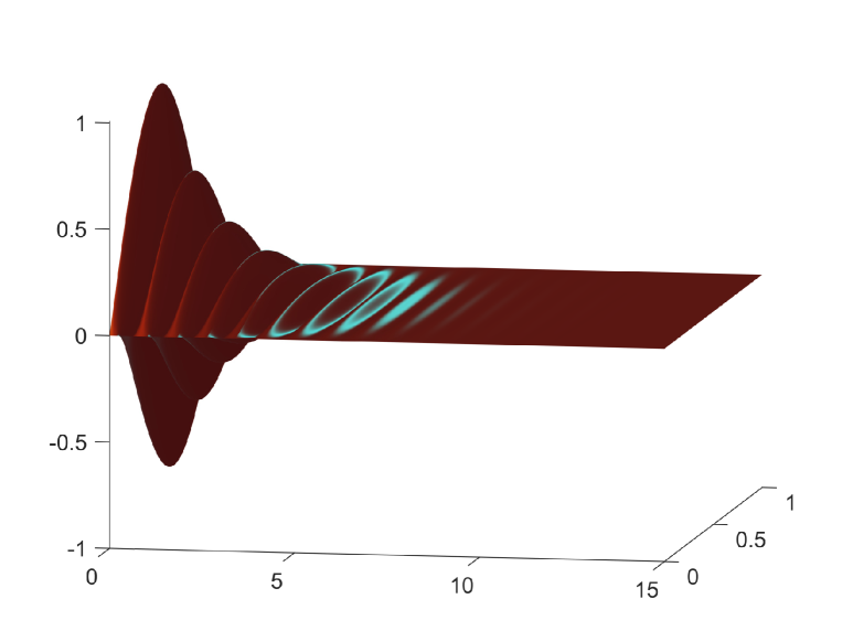
Figure 1. The evolution in time and space of $u$.

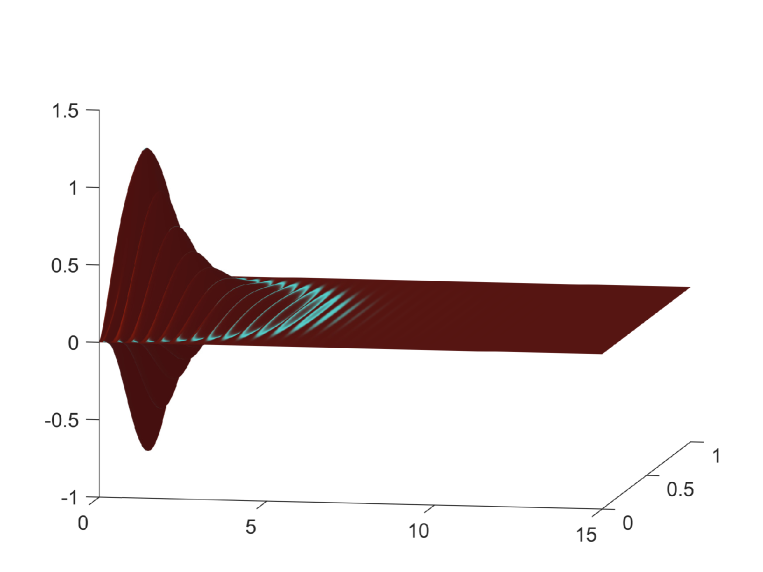
Figure 2. The evolution in time and space of $\varphi$.

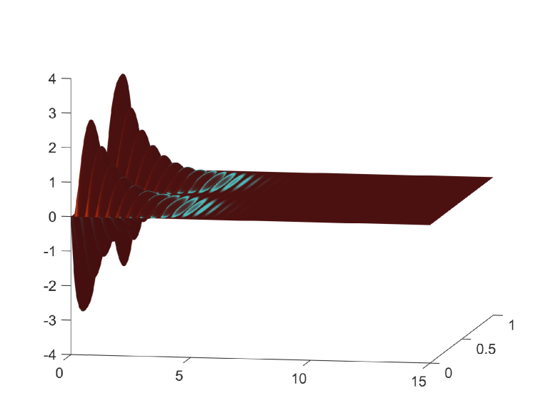
Figure 3. The evolution in time and space of $\psi$.

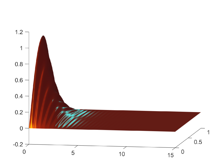
Figure 4. The evolution in time and space of $w$.

The results at point $x=0.6$ are displayed in Figures 5, 6 and 7.

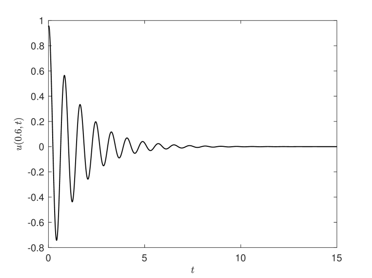
Figure 5. The evolution in time of $u$ at $x=0.6$.

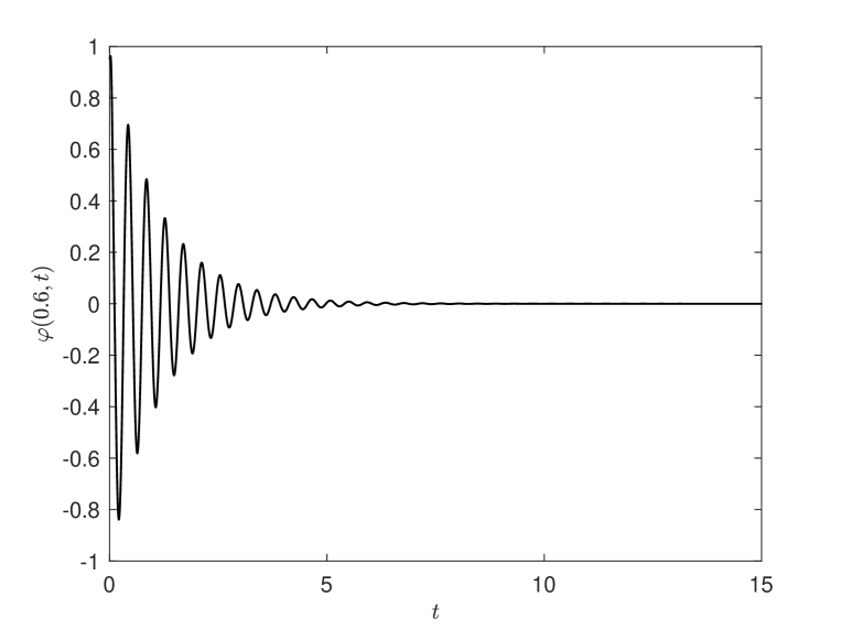
Figure 6. The evolution in time of $\varphi$ at $x=0.6$.

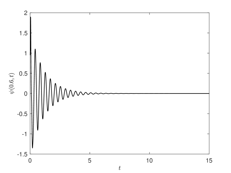
Figure 7. The evolution in time of $\psi$ at $x=0.6$.

The decay of energy with respect to time is shown in Figures 8, 9 and 10.

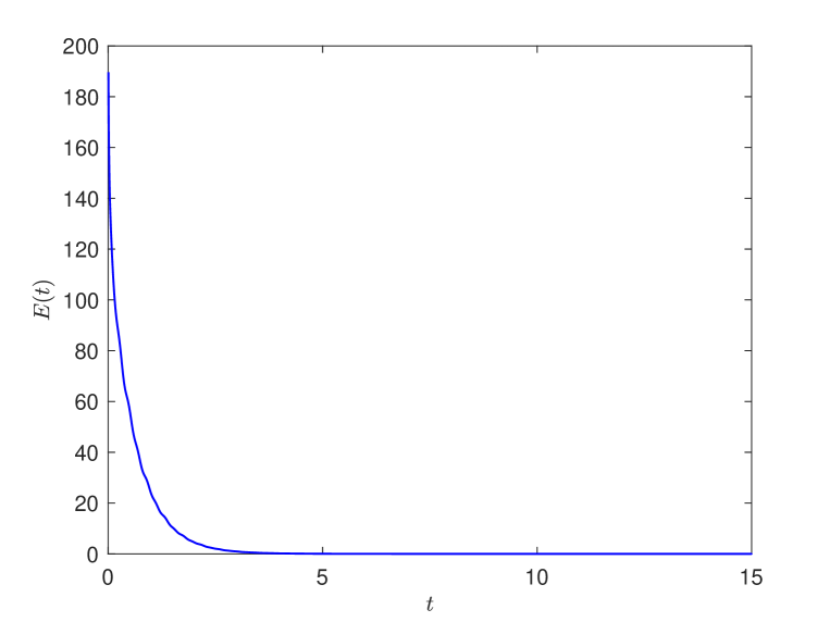
Figure 8. The evolution in time of energy $E$.

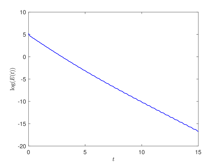
Figure 9. The evolution in time of $\log(E(t))$.

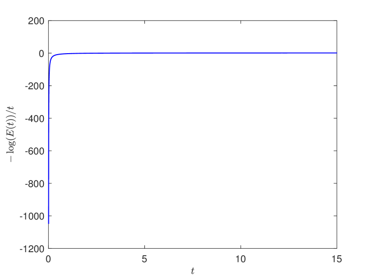
Figure 10. The evolution in time of $-\log(E(t))/t$.

Following this, we carried out a numerical simulation to evaluate the accuracy of the error estimate. We solved the modified problem

$$\begin{cases}\rho u_{tt}-\alpha u_{xx}-\lambda\left(\varphi-u\right)+\mu u_{t}=f_{1},\\ \rho_{1}\varphi_{tt}-K\left(\varphi_{x}+\psi\right)_{x}+\lambda\left(\varphi-u\right)+\gamma\varphi_{t}+\beta w_{xt}=f_{2},\\ -b\psi_{xx}+K\left(\varphi_{x}+\psi\right)=f_{3},\\ \rho_{3}w_{tt}-\delta w_{xx}+\beta\varphi_{xt}-\kappa w_{xxt}=f_{4},\\ \end{cases}$$ (6.1)

where functions $f_{1}$, $f_{2}$, $f_{3}$, $f_{4}$, and the initial data are derived from the exact solution

$$\begin{split}u(x,t)&=0.01tx^{2}(x-1)^{2},\\ \varphi(x,t)&=e^{t}\sin(\pi x),\\ \psi(x,t)&=e^{t}x\cos(0.5\pi x),\\ w(x,t)&=2e^{t}\sin(\pi x).\\ \end{split}$$

The calculated errors at time $t=1.2$ are presented in Table 1, where the $Error$ is defined as

$$\begin{split}Error=&(\rVert\xi^{n}_{h}-\xi(t_{n})\lVert^{2}+\rVert u^{n}_{hx}-(u(t_{n}))_{x}\lVert^{2}+\rVert\varphi^{n}_{h}-u^{n}_{h}-(\varphi(t_{n})-u(t_{n}))\lVert^{2}\\ &+\rVert\Phi^{n}_{h}-\Phi(t_{n})\lVert^{2}+\rVert\varphi^{n}_{hx}+\psi^{n}_{h}-((\varphi(t_{n}))_{x}+\psi(t_{n}))\lVert^{2}+\rVert\psi^{n}_{hx}-(\psi(t_{n}))_{x}\lVert^{2}\\ &+\rVert\vartheta^{n}_{h}-\vartheta(t_{n})\lVert^{2}+\rVert w^{n}_{hx}-(w(t_{n}))_{x}\lVert^{2})^{\frac{1}{2}}.\end{split}$$

It can be observed that the errors decrease by a factor of approximately 2 when the discretization parameters are halved. The linear convergence rate is also evident in the curves illustrated in Figure 11.

Table 1. Computed errors when $T=1.2$.

$M$	$\Delta t$	$Error$
$40$	$1.00\times 10^{-3}$	$4.164\times 10^{-1}$
$80$	$5.00\times 10^{-4}$	$1.949\times 10^{-1}$
$160$	$2.50\times 10^{-4}$	$9.567\times 10^{-2}$
$320$	$1.25\times 10^{-4}$	$4.770\times 10^{-2}$
$640$	$6.25\times 10^{-5}$	$2.402\times 10^{-2}$
$1280$	$3.125\times 10^{-5}$	$1.241\times 10^{-2}$

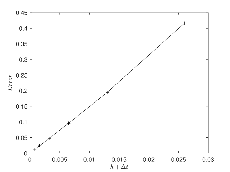
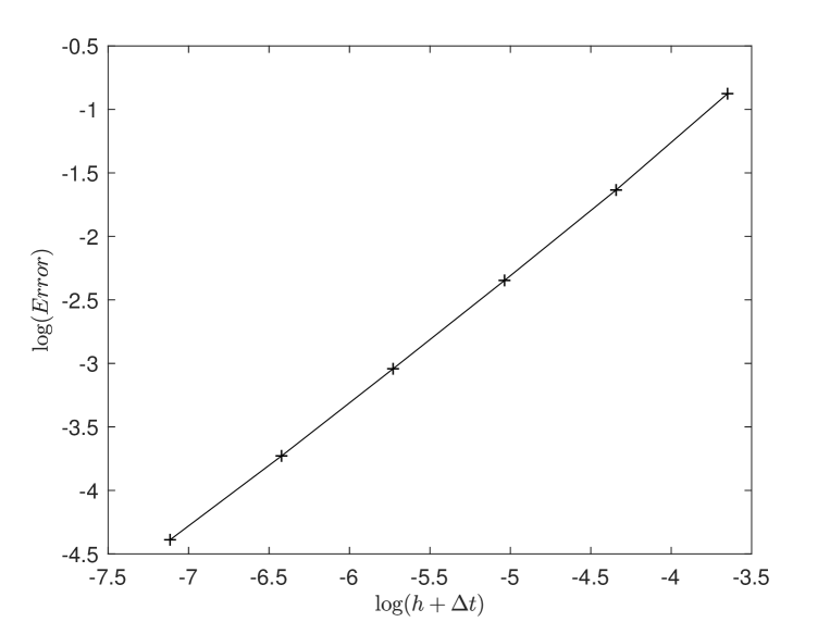
Figure 11. The evolution of the error depending on $h+\Delta t$.

References

- [1] A. M. Abdel-Ghaffar, Vertical vibration analysis of suspension bridges, ASCE J. Stru. Div. 108 (1980), no. 10, 2053–2075.
- [2] A. M. Abdel-Ghaffar, L. I. Rubin, Non linear free vibrations of suspension bridges: theory, ASCE J. Eng. Mech. 109 (1983) 313–329.
- [3] A. M. Abdel-Ghaffar, L. I. Rubin, Non linear free vibrations of suspension bridges: application, ASCE J. Eng. Mech. 109 (1983) 330–345.
- [4] N. U. Ahmed, H. Harbi, Mathematical analysis of dynamic models of suspension bridges, SIAM J. Appl. Math. 109 (1998) 853–874.
- [5] D. S. Almeida Júnior, A. J. A. Ramos, On the nature of dissipative Timoshenko systems at light of the second spectrum, Z. Angew. Math. Phys. 68 (145) (2017).
- [6] D. S. Almeida Júnior, A. J. A. Ramos, M. M. Freitas, Energy decay for damped Shear beam model and new facts related to the classical Timoshenko system, Appl. Math. Lett. 120 (2021), 107324, 7 pp.
- [7] D. N. Arnold, A. L. Madureira, S. Zhang, On the range of applicability of the Reissner-Mindlin and Kirchhoff-Love plate bending models, J. Elast. Phys. Sci. Solids 67 (2002), no. 3, 171–185.
- [8] C. Bernardi, M. I. M. Copetti, Discretization of a nonlinear dynamic thermoviscoelastic Timoshenko beam model, Z. Angew. Math. Mech. 97 (2017) 532–549.
- [9] I. Bochicchio, M. Campo, J. R. Fernández, M. G. Naso, Analysis of a thermoelastic Timoshenko beam model, Acta Mech. 231 (2020) 4111–4127.
- [10] I. Bochicchio, C. Giorgi, E. Vuk, Long-term dynamics of the coupled suspension bridge system, Math. Models Methods Appl. Sci. 22 (2012) 1250021, 22 pp.
- [11] I. Bochicchio, C. Giorgi, E. Vuk, Asymptotic dynamics of nonlinear coupled suspension bridge equations, J. Math. Anal. Appl. 402 (2013) 319–333.
- [12] I. Bochicchio, C. Giorgi, E. Vuk, Long-term dynamics of a viscoelastic suspension bridge, Meccanica 49(9) (2014) 2139–2151.
- [13] I. Bochicchio, C. Giorgi, E. Vuk, Buckling and nonlinear dynamics of elastically-coupled double-beam systems, Int. J. Nonlinear Mech. 85 (2016) 161–177.
- [14] F. Boyer, P. Fabrie, Mathematical tools for the study of the incompressible Navier-Stokes equations and related models, Applied Mathematical Sciences, Springer, New York, 2013.
- [15] C. Cattaneo, On a form of heat equation which eliminates the paradox of instantaneous propagation, C. R. Acad. Sci. Paris, 247 (1958) 431–433.
- [16] D. S. Chandrasekharaiah, A note on uniqueness of solution in the linear theory of thermoelasticity without energy dissipations, J. Thermal Stresses 19 (1996) 695–710.
- [17] D. S. Chandrasekharaiah, Complete solutions in the theory of thermoelasticity without energy dissipations, Mech. Res. Commun. 24 (1997) 625–630.
- [18] L. Djilali, A. Benaissa, A. Benaissa, Global existence and energy decay of solutions to a viscoelastic Timoshenko beam system with a nonlinear delay term, Appl. Anal. 95 (2016) 2637–2660.
- [19] P. Drábek, G. Holubová, A. Matas, P. Nečesal, Nonlinear models of suspension bridges: discussion of the results, Appl. Math. 48 (2003) 497–514.
- [20] T. El Arwadi, M. I. M. Copetti, W. Youssef, On the theoretical and numerical stability of the thermoviscoelastic Bresse system, Z. Angew. Math. Mech. 99 (10) (2019) 1–20.
- [21] A. E. Green, P. E. Naghdi, A re-examination of the basic postulates of thermomechanics, Proc. Royal Society London, A 432 (1991) 174–194.
- [22] A. E. Green, P. M. Naghdi, On undumped heat waves in elastic solid, J. Thermal Stresses 15 (1992) 253–264.
- [23] A. E. Green, P. E. Naghdi, Thermoelasticity without energy dissipassion, J. Elasticity 91 (1993) 189–208.
- [24] T. Hayashikawa, N. Watanabe, Vertical vibration in Timoshenko beam suspension bridges, J. Eng. Mech. 110 (1984), no. 3, 341–356.
- [25] A. Labuschagne, N. F. J. van Rensburg, A. J. van der Merwe, Comparison of linear beam theories, Math. Comput. Model. 49 (2009) 20–30.
- [26] A. C. Lazer, P. J. McKenna, Existence and stability of large-scale nonlinear oscillations in suspension bridge, Z. Angew. Math. Phys. 40 (1989) 171–200.
- [27] A. C. Lazer, P. J. McKenna, Large-amplitude periodic oscillations in suspension bridges: some new connections with nonlinear analysis, SIAM Rev. 32 (1990) 537–578.
- [28] J. L. Lions, E. Magenes, Problèmes aux Limites non Homogènes, Aplications, Dunod, Paris, 1968.
- [29] S. A. Messaoudi and B. Said-Houari, Energy decay in Timoshenko-type system of thermoelasticity of type III, J. Math. Anal. Appl. 384 (2008) 298–307.
- [30] S. E. Mukiawa, Y. Khan , H. Al Sulaimani, M. E. Omaba, C. D. Enyi, Thermal Timoshenko beam system with suspenders and Kelvin-Voigt damping, Front. Appl. Math. Stat. 9 (2023), 1153071, 7 pp.
- [31] S. E. Mukiawa, M. Leblouba, S. A. Messaoudi, On the well-posedness and stability for a coupled nonlinear suspension bridge problem, Commun. Pure Appl. Anal. 22(9) (2023) 2716–2743.
- [32] R. Quintanilla, R. Racke, Stability in thermoelasticity of type III, Discrete Contin. Dyn. Syst. Ser. B 3 (2003) 383–400.
- [33] A. J. A. Ramos, D. S. A. Júnior, M. M. Freitas, About well-posedness and lack of exponential stability of Shear beam models, Ann. Univ. Ferrara 68 (2022) 129–136.
- [34] S. P. Timoshenko, On the correction for shear of the differential equation for transverse vibrations of prismatic bars, Phil. Mag. 6 (41/245) (1921) 744–746.
- [35] X. Zhang, E. Zuazua, Decay of solutions of the system of thermoelasticity of type III, Commun. Contemp. Math. 5(1) (2003) 25–83.