Every circle homeomorphism is the composition of two weldings

Abstract.

We show that every orientation-preserving circle homeomorphism is a composition of two conformal welding homeomorphisms, which implies that conformal welding homeomorphisms are not closed under composition. Our approach uses the log-singular maps introduced by Bishop. The main tool that we introduce are log-singular sets, which are zero capacity sets that admit a log-singular map that maps their complement to a zero capacity set.

1. Introduction

Let $\gamma\subset\mathbb{C}_{\infty}$ be a Jordan curve and consider $\Omega,\Omega^{*}$ the two complementary components of $\gamma$ in $\mathbb{C}_{\infty}$, the Riemann sphere. By the Riemann mapping theorem there are conformal maps $f\colon\mathbb{D}\to\Omega$ and $g\colon\mathbb{C}_{\infty}\setminus\overline{\mathbb{D}}=\mathbb{D}^{*}\to\Omega^{*}$, as represented in Figure 1. By the Carathéodory-Torhorst theorem, these conformal maps extend to be homeomorphisms of the unit circle to $\gamma$. This yields the orientation-preserving homeomorphism $h=g^{-1}\circ f\colon\mathbb{S}^{1}\to\mathbb{S}^{1}$ which we call a conformal welding (or welding for short).

It is well known that there are orientation-preserving circle homeomorphisms that are not weldings. For instance, Oikawa provided in [Oik61, Example 1] a family of such examples that are biHölder. However, well-behaved self-maps of the circle, like quasisymmetric maps, are weldings. This is the so called fundamental theorem of conformal welding and it was first proven by Pfluger in [Pfl60] by using the measurable Riemann mapping theorem. Shortly after, Lehto and Virtanen [LV60] gave a different proof, also by using quasiconformal mappings.

In this paper we prove that every orientation-preserving circle homeomorphism is a composition of two conformal welding homeomorphisms.

Theorem 1.1 (Every circle homeomorphism is the composition of two weldings).

Let $\phi\colon\mathbb{S}^{1}\to\mathbb{S}^{1}$ be an orientation-preserving circle homeomorphism, then there exist conformal weldings $\varphi$ and $\psi$ so that $\phi=\varphi\circ\psi$.

In particular, weldings are not closed under composition.

Corollary 1.2.

The set of conformal welding homeomorphisms is not closed under composition.

While it was generally believed that the set of weldings is not closed under composition, our construction appears to be the first example. However, as we will point out later in the introduction, this followed from some previous work of Bishop [Bis07] and the examples provided by Oikawa [Oik61].

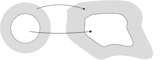
Figure 1. Definition of conformal welding. The conformal maps $f$ and $g$ map the interior and exterior of the unit circle to the two complementary components of a Jordan curve $\gamma$.

This means that the structure of the space of weldings is an intricate object. There have been some important breakthroughs regarding conformal weldings, like Bishop’s paper [Bis07], in which he proves that a very badly behaved class of circle homeomorphisms are weldings. Some work from Astala, Jones, Kupiainen and Saksman [AJKS11] proves that regularity at most scales is a sufficient condition for an homeomorphism to be a welding (which is satisfied for quasisymmetric maps). However, many important questions are still open, like showing whether or not the collection of weldings is a Borel subset of the space of circle homeomorphisms. In [Bis20, Section 9] Bishop proves that it is at least analytic. He also raises several questions regarding weldings and their relations to other problems in geometric function theory.

Conformal welding has also been used in many other areas of mathematics. For example, Sheffield [She16] and Duplantier, Miller and Sheffield [DS11] used conformal welding to relate Liouville quantum gravity and Schramm-Loewner evolution curves. See also Ang, Holden and Sun [AHS23], where they prove that SLE_κ measure, for $\kappa\in(0,4)$, arises naturally from the conformal welding of two $\sqrt{\kappa}$-Liouville quantum gravity disks. Sharon and Mumford [SM06] used conformal welding in their applications to computer vision.

What maps can be used to prove Theorem 1.1? Well-behaved classes of homeomorphisms, like diffeomorphisms, biLipschitz maps, quasisymmetric maps and biHölder maps, cannot be used since they each form a proper subgroup of the group of circle homeomorphisms. However, there are circle homeomorphisms with arbitrarily bad modulus of continuity.

We say that a circle homeomorphism $h\colon\mathbb{S}^{1}\to\mathbb{S}^{1}$ is log-singular if there is a (logarithmic) zero capacity Borel set $E\subset\mathbb{S}^{1}$ so that $h(\mathbb{S}^{1}\setminus E)$ has zero capacity. Log-singular maps are stronger versions of the better known singular maps $\phi$ so that $\phi^{\prime}=0$ a.e., since they map a set of full Lebesgue measure to a measure zero set. One of the main results obtained in [Bis07] is that log-singular homeomorphisms are weldings.

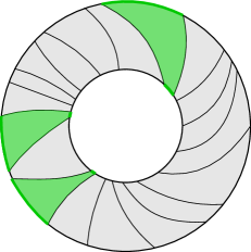
Figure 2. Representation of a log-singular circle homeomorphism $h\colon\mathbb{S}^{1}\to\mathbb{S}^{1}$. The arcs $I_{j}$, which have small capacity, are mapped to the arcs $h(I_{j})$, which have larger capacity.

Theorem 1.3 ([Bis07] Theorem 3).

Every log-singular circle homeomorphism $h\colon\mathbb{S}^{1}\to\mathbb{S}^{1}$ is a conformal welding homeomorphism.

In light of Theorem 1.3, we see that Theorem 1.1 reduces to proving that any circle orientation-preserving circle homeomorphism is a composition of two log-singular maps.

Theorem 1.4 (Circle homeomorphisms and log-singular homeomorphisms).

Let $\phi\colon\mathbb{S}^{1}\to\mathbb{S}^{1}$ be a circle homeomorphism, then there exists a log-singular map $h\colon\mathbb{S}^{1}\to\mathbb{S}^{1}$ so that $\phi\circ h^{-1}$ is also log-singular. Thus $\phi=(\phi\circ h^{-1})\circ h$ is a composition of two welding maps.

Observe that Theorem 1.4 follows immediately from Theorem 1.3 if the circle homeomorphism $\phi$ has enough regularity. For instance, biHölder homeomorphisms preserve zero capacity sets. Therefore, if $\phi\colon\mathbb{S}^{1}\to\mathbb{S}^{1}$ is biHolder, then $\phi\circ h^{-1}$ is log-singular for any log-singular circle homeomorphism $h\colon\mathbb{S}^{1}\to\mathbb{S}^{1}$. Since $\phi=(\phi\circ h^{-1})\circ h$, and $\phi\circ h^{-1}$ and $h$ are weldings by Theorem 1.3, every biHölder circle homeomorphism is a composition of two weldings. The examples of non-welding homeomorphisms provided by Oikawa [Oik61, Example 1] are biHölder, hence weldings are not closed under composition (Corollary 1.2). Similarly, any circle homeomorphism that preserves sets of zero capacity is also a composition of two (log-singular) weldings. The novel aspect of this paper is to prove that this holds for all (orientation-preserving) circle homeomorphisms.

Given any circle homeomorphism $\phi$, it suffices to build a log-singular homeomorphism $h$ and a set $E$ of zero capacity so that both $h(\mathbb{S}^{1}\setminus E)$ and $\phi(E)$ have zero capacity, for then $\phi\circ h^{-1}$ and $h$ are log-singular. The set $E$ that we will construct will be a countable union of Cantor sets, and it will be described using an infinite tree whose vertices are labeled by finite strings of integers (which we call addresses), much like a binary tree represents dyadic intervals. In our case, the number of children of a vertex increases in each generation, and, unlike the dyadic case, intervals in the same generation may have very different sizes.

By using addresses we provide a large class of zero capacity sets $E$, so that there exists a log-singular homeomorphism $h\colon\mathbb{S}^{1}\to\mathbb{S}^{1}$ with $h(\mathbb{S}^{1}\setminus E)$ of zero capacity, which we call a log-singular set. In fact, any log-singular map admits as a log-singular set one of the zero capacity sets that we construct.

The paper is structured in the following way.

Section 2: We introduce logarithmic capacity and summarize some known properties. We also introduce flexible curves and summarize the relevant results from [Bis07].

Section 3: We introduce log-singular sets and addresses, which encode partitions of a given interval or arc. We use addresses to build log-singular sets and log-singular maps.

Section 4: We prove that given a circle homeomorphism $\phi$ there is a log-singular set $E\subset\mathbb{S}^{1}$, given by an address, so that $\operatorname{Cap}(\phi(E))=0$. We also prove Theorem 1.4.

Acknowledgements

I would like to thank Chris Bishop for his continued guidance and support, and for reading (many) drafts of the paper which highly improved the presentation via his comments, suggestions and remarks. Spencer Cattalani has pointed out many typos and grammatical mistakes. Steffen Rohde and Yilin Wang have pointed applications of conformal welding to Liouville quantum gravity and Schramm-Loewner evolution curves. Steffen Rohde has also pointed out some typos and suggested highlighting more that weldings are not closed under composition.

2. Preliminaries

In this section we summarize known results regarding (logarithmic) capacity that we will use in the following sections. The results have been obtained from the books of Carleson, Garnett and Marshall, and Pommerenke [Car67, GM08, Pom92]. We also recall the definition of quasisymmetric homeomorphisms and provide a summary of the main results obtained by Bishop in [Bis07].

2.1. Logarithmic capacity

Let $\mu$ be a finite compactly supported signed (Borel) measure. The logarithmic potential of $\mu$ is the functional

$$U_{\mu}(z)=\int\log\frac{1}{|\xi-z|}d\mu(\xi).$$

By Fubini’s theorem, $U_{\mu}(z)$ is finite a.e. with respect to Lebesgue measure. If

$$\iint\left|\log\frac{1}{|z-\xi|}\right|d|\mu|(\xi)d|\mu|(z)<\infty,$$

we say that $\mu$ has finite energy and define the energy integral $I(\mu)$ by

$$I(\mu)=\iint\log\frac{1}{|z-\xi|}d\mu(\xi)d\mu(z)=\int U_{\mu}(z)d\mu(z).$$

Let $K$ be compact and denote by $P(K)$ the set of all Borel probability measures on $K$. Define the Robin’s constant of $K$ by

$$\gamma(K)=\inf\{I(\mu)\colon\mu\in P(K)\},$$

and the (logarithmic) capacity of $K$ by

$$\operatorname{Cap}(K)=e^{-\gamma(K)}.$$

It follows that $\gamma(K)<\infty$ if and only if $\operatorname{Cap}(K)>0$, which holds as long as there is a probability $\mu\in P(K)$ with finite energy $I(\mu)<\infty$. If $K_{1}\subset K_{2}$, then any probability on $K_{1}$ is also a probability on $K_{2}$. Hence $\gamma(K_{1})\geq\gamma(K_{2})$ and $\operatorname{Cap}(K_{1})\leq\operatorname{Cap}(K_{2})$, i.e. the capacity set function is increasing with respect to set inclusion.

The capacity of any Borel set $E$ is defined as

$$\operatorname{Cap}(E)=\sup\{\operatorname{Cap}(K)\colon K\textrm{ compact},K\subset E\}.$$

Capacity can be a difficult object to compute, but the capacities of some simple sets are know (see [GM08, Chapter 3] or [Pom92, Chapter 9]). For example, for $a,b\in\mathbb{C}$, $\operatorname{Cap}[a,b]=|a-b|/4$, and the capacity of a disk is its radius, i.e. $\operatorname{Cap}(\mathbb{D}(a,r))=r$.

We now summarize some other known (important) properties of logarithmic capacity that we will need later.

Proposition 2.1.

Logarithmic capacity satisfies the following properties.

1. If $\varphi$ is $L$-Lipschitz, then $\operatorname{Cap}(\varphi(E))\leq L\operatorname{Cap}(E)$.

2. If $h(\xi)=c\xi+c_{0}+c_{1}\xi^{-1}+\cdots$ maps $\mathbb{C}_{\infty}\setminus\overline{\mathbb{D}}$ conformally onto $G$ then $\operatorname{Cap}(\partial G)=|c|$.

3. Borel sets are capacitable, that is, given $E$ Borel and $\varepsilon>0$, there is an open set $V$ with $E\subset V$ and $\operatorname{Cap}(V)<\operatorname{Cap}(E)+\varepsilon$.

4. Let $E_{n}$ be Borel sets and $E=\cup_{n=1}^{\infty}E_{n}$. If $\operatorname{diam}(E)<b$ then

   $$1/\log\frac{b}{\operatorname{Cap}(E)}\leq\sum_{n}1/\log\frac{b}{\operatorname{Cap}(E_{n})}.$$

   In particular, the union of countably many sets of zero capacity has zero capacity.

5. If $E_{n}$ are Borel sets so that $E=\cup E_{n}$ has diameter less or equal than one, then $\operatorname{Cap}(E)\leq\sum\operatorname{Cap}(E_{n})$.

The proof of (1), (2), (3) and (4) can be found in [Pom92, Chapter 9], (4) is also Theorem 7 from [Car67, Section 3]. (5) follows from Lemma 4 in [Car67, Section 3].

We say that a circle homeomorphism $\phi\colon\mathbb{S}^{1}\to\mathbb{S}^{1}$ is $\alpha$-biHolder if there is a constant $C>0$ so that

$$\frac{1}{C}|z-w|^{1/\alpha}\leq|\phi(z)-\phi(w)|\leq C|z-w|^{\alpha}.$$

As it was already mentioned in the introduction, biHolder maps preserve sets of zero capacity.

Lemma 2.2.

Let $\phi$ be $\alpha$-biHolder, then $\operatorname{Cap}(E)=0$ if and only if $\operatorname{Cap}(\phi(E))=0$.

2.2. Quasisymmetric homeomorphisms

We say that a circle homeomorphism $\phi\colon\mathbb{S}^{1}\to\mathbb{S}^{1}$ is quasisymmetric if there is a constant $M<\infty$ so that

$$M^{-1}\leq|\phi(I)|/|\phi(J)|\leq M,$$

whenever $I,J\subset\mathbb{S}^{1}$ are two adjacent arcs of equal length (see [Ahl06, AIM09, LV73] for more information regarding quasisymmetric homeomorphisms).

Pfluger proved that quasisymmetric homeomorphisms are weldings.

Theorem 2.3 (Pfluger [Pfl60]).

Every quasisymmetric circle homeomorphism is a conformal welding.

By [AIM09, Corollary 3.10.3], every quasisymmetric circle homeomorphism is $\alpha$-biHolder for some $\alpha>0$. Therefore quasisymmetric circle homeomorphisms preserve sets of zero capacity.

2.3. Flexible curves and log-singular homeomorphisms

In [Bis94] Bishop introduced and proved the existence of flexible curves. We say that a Jordan curve $\gamma\subset\mathbb{C}$ is flexible if the following conditions are satisfied:

1. Given any other Jordan curve $\tilde{\gamma}$ and any $\varepsilon>0$, there exists a homeomorphism $\phi\colon\mathbb{C}_{\infty}\to\mathbb{C}_{\infty}$, conformal off $\gamma$, so that the Hausdorff distance between $\phi(\gamma)$ and $\tilde{\gamma}$ is less than $\epsilon$.

2. Given $z_{1},z_{2}$ in each component of $\mathbb{C}_{\infty}\setminus\gamma$ and $w_{1},w_{2}\in\mathbb{C}_{\infty}\setminus\tilde{\gamma}$, the previous $\phi$ can be taken so that $\phi(z_{j})=w_{j}$ for $j=1,2$.

Flexible curves are conformally non-removable in a very strong sense. Later in [Bis07] Bishop proved that $h\colon\mathbb{S}^{1}\to\mathbb{S}^{1}$ is the conformal welding of a flexible curve if and only if it is log-singular. The specific statement that he proved is the following, which implies Theorem 1.3.

Theorem 2.4 ([Bis07] Theorem 3).

Let $h\colon\mathbb{S}^{1}\to\mathbb{S}^{1}$ be a log-singular homeomorphism with $h(1)=1$, and let $f_{0},g_{0}$ be two conformal maps of $\mathbb{D}$ and $\mathbb{C}_{\infty}\setminus\overline{\mathbb{D}}$ respectively onto disjoint domains. Then, for any $0<r<1$ and any $\varepsilon>0$, there are conformal maps $f$ and $g$ of $\mathbb{D}$ and $\mathbb{C}_{\infty}\setminus\overline{\mathbb{D}}$ onto the two complementary components of a Jordan curve $\gamma$ that satisfy:

1. $h=g^{-1}\circ f$ on $\mathbb{S}^{1}$, i.e. $h$ is a conformal welding.

2. $|f(z)-f_{0}(z)|<\varepsilon$ for all $|z|\leq r$.

3. $|g(z)-g_{0}(z)|<\varepsilon$ for all $|z|\geq 1/r$.

Moreover, the curve $\gamma$ can be taken to have zero area.

Theorem 1.1 (and Theorem 1.4), that we prove in this paper, shows that any circle homeomorphism can be written as a composition of two weldings. In [Bis07] Bishop proved that every circle homeomorphism is a welding on a set of nearly full measure.

Theorem 2.5 ([Bis07] Theorem 1).

Given any orientation-preserving homeomorphism $\phi\colon\mathbb{S}^{1}\to\mathbb{S}^{1}$ and $\varepsilon>0$, there are a set $E\subset\mathbb{S}^{1}$ with $|E|+|h(E)|<\varepsilon$ and a conformal welding homeomorphism $h\colon\mathbb{S}^{1}\to\mathbb{S}^{1}$ such that $\phi(x)=h(x)$ for all $x\in\mathbb{S}^{1}\setminus E$.

3. Log-singular sets and addresses

In this section, we prove that log-singular maps and log-singular sets exist in Lemma 3.2 and Corollary 3.5. We give sufficient conditions for a zero capacity set $E$ to admit a log-singular homeomorphism $h$ satisfying $\operatorname{Cap}(h(\mathbb{S}^{1}\setminus E))=0$, which we call a log-singular set. The approach is based on what we call addresses, which encode partitions of a fixed arc of $\mathbb{S}^{1}$ (or an interval) by sub-arcs (or sub-intervals) in an iterative way.

We proceed to define addresses. It suffices to do so for $I=[0,1]$, since the definition will work for any other interval or sub-arc of $\mathbb{S}^{1}$ in an analogous way.

Let $\{L_{n}\}_{n\geq 0}$ be a sequence of positive integers with $L_{0}=1$. We say that $A_{n}=\{a_{1},a_{2},\ldots,a_{n}\}$, where $0\leq a_{j}<L_{j}$ for $1\leq j\leq n$, is a word of length $n$. Suppose that for $n\geq 1$ we have have intervals $I_{A_{n}}\subset[0,1]$ that satisfy:

1. If $n\leq m$ and $A_{n}=\{a_{1},a_{2},\ldots,a_{n}\}$, $\tilde{A}_{m}=\{\tilde{a}_{1},\ldots,\tilde{a}_{n},\ldots,\tilde{a}_{m}\}$, then $I_{\tilde{A}_{m}}\subset I_{A_{n}}$ if and only if $a_{j}=\tilde{a}_{j}$ for $1\leq j\leq n$ (in such a case, $A_{n}$ is often called the prefix of $\tilde{A}_{m}$).

2. If $A_{n}\not=\tilde{A}_{n}$, then $I_{A_{n}}$ and $I_{\tilde{A}_{n}}$ have disjoint interiors.

3. $L_{n}$ denotes the number of intervals in which each $I_{A_{n-1}}$ has been divided, which we assume is the same for all $I_{A_{n-1}}$.

4. For each $n$, the union over all possible $I_{A_{n}}$ is $I$. Moreover, if we fix a word $A_{n-1}=\{a_{1},\ldots,a_{n-1}\}$, then the union over all possible $A_{n}=\{a_{1},\ldots,a_{n-1},a\}$, with $0\leq a<L_{n}$, is $I_{A_{n-1}}$, i.e.

   $$I_{A_{n-1}}=\bigcup_{0\leq a<L_{n}}I_{\displaystyle\{a_{1},\ldots,a_{n-1},a\}}.$$

We will say that $A_{n}$ is the address of $I_{A_{n}}$; $A_{n}$ represents the directions that we need to take in the decomposition to reach $I_{A_{n}}$, in the sense that if we fix $A_{n}=\{a_{1},\ldots,a_{n}\}$, then

$$I_{A_{n}}=\bigcap_{j=1}^{n}I_{\{a_{1},\ldots,a_{j}\}}.$$

Figure 3. Addresses associated to a partition of an interval $I$ with $L_{1}=3,L_{2}=5,L_{3}=4,L_{4}=2,L_{5}=3$. The address to $I_{\{1,3,0,1,2\}}$ is highlighted in a lighter color and by dashed arrows.

This is illustrated in Figure 3. If $A_{n-1}=\{a_{1},\ldots,a_{n-1}\}$ we will also set, for $0\leq a<L_{n}$, $A_{n-1}(a)=\{a_{1},\ldots,a_{n-1},a\}$ to denote that we extend the word $A_{n-1}$ by $a$.

Similarly, given an infinite sequence $\{a_{j}\}_{j\in\mathbb{N}}$, with $0\leq a_{j}<L_{j}$ for each $j\in\mathbb{N}$, we denote $A_{\infty}=\{a_{1},a_{2},\ldots\}$. Observe that given $A_{\infty}=\{a_{1},a_{2},\ldots\}$, then

$$I_{A_{\infty}}=\bigcap_{n\geq 1}I_{\{a_{1},\ldots,a_{n}\}}$$

is either an interval or a point (since the lengths of the intervals decrease with $n$). If for any $\varepsilon>0$, there exists $N\geq 1$ so that for every $n\geq N$ we have $|I_{A_{n}}|<\varepsilon$, then $I_{A_{\infty}}$ is a singleton.

We will denote by $\mathcal{A}_{n}$ the collection of all possible words $A_{n}$ of length $n$, and by $\mathcal{A}_{\infty}$ the collection of all possible words $A_{\infty}$.

Well-known examples of such partitions include the usual binary or decimal representations of real numbers. For example, the dyadic partition of $[0,1]$ is given, in terms of addresses, by taking the sequence $\{L_{n}\}$ of positive integers with $L_{0}=1$ and $L_{n}=2$ for $n\geq 1$. Each interval $I_{A_{n}}$ is split into two intervals of equal length (observe that the length of each $I_{A_{n}}$ is $2^{-n}$). We define the dyadic partition of an interval $I=[a,b]$ as the partition given by the collection of intervals $\{I_{A_{n}}\}$ so that fixed $n$,

$$I_{A_{n}}\subset\left\{\left[a+\frac{j}{2^{n}},a+(b-a)\frac{j+1}{2^{n}}\right]\colon 0\leq j<2^{n}\right\}.$$

We recall the definition of log-singular homeomorphisms and log-singular sets.

Definition 3.1 (Log-singular homeomorphism, log-singular set).

Let $I,J$ be two subarcs of $\mathbb{S}^{1}$. An orientation-preserving homeomorphism $h\colon I\to J$ is log-singular if there exists a Borel set $E\subset I$ such that both $E$ and $h(I\setminus E)$ have zero logarithmic capacity. We say that a Borel set $E\subset\mathbb{S}^{1}$ is a log-singular set if $\operatorname{Cap}(E)=0$ and there exists a log-singular homeomorphism $h\colon\mathbb{S}^{1}\to\mathbb{S}^{1}$ so that $\operatorname{Cap}(h(\mathbb{S}^{1}\setminus E))=0$.

Observe that if $h\colon\mathbb{S}^{1}\to\mathbb{S}^{1}$ is a log-singular map with log-singular set $E\subset\mathbb{S}^{1}$, then $h(\mathbb{S}^{1}\setminus E)$ is also a log-singular set.

We can now prove that log-singular sets and log-singular maps exist. We will do so by using addresses, provided that we can obtain a dense capacity zero set.

Lemma 3.2 (Log-singular sets and addresses).

Let $I,J$ be two subarcs of $\mathbb{S}^{1}$, and let $\{L_{n}\}$ be a sequence of positive integers so that $L_{0}=1$ and $L_{n}$, for $n\geq 1$, is an even number. Consider words $A_{n}=\{a_{1},a_{2},\ldots,a_{n}\}$ with $0\leq a_{j}<L_{j}$. Suppose that $\{I_{A_{n}}\}$ is a partition of $I=I_{A_{0}}$ and $\{J_{A_{n}}\}$ is a partition of $J=J_{A_{0}}$ satisfying that given $\varepsilon>0$, there exists $N\geq 1$ such that for every $n\geq N$, $|I_{A_{n}}|+|J_{A_{n}}|<\varepsilon$. Define

$$E=\bigcap_{n\in\mathbb{N}}\bigcup_{m\geq n}\left(\bigcup_{A_{m}\in\mathcal{A}_{m}}\bigcup_{j=1}^{L_{m+1}/2}I_{A_{m}(2j-1)}\right)$$

and

$$F=\bigcup_{n\in\mathbb{N}}\bigcap_{m\geq n}\left(\bigcup_{A_{m}\in\mathcal{A}_{m}}\bigcup_{j=1}^{L_{m+1}/2}J_{A_{m}(2j-2)}\right).$$

If $\operatorname{Cap}(E)=0$ and $\operatorname{Cap}(F)=0$, then $E$ and $F$ are log-singular sets and there exists a log-singular map $h\colon I\to J$ so that $h(\mathbb{S}^{1}\setminus E)=F$.

Remark 3.3.

In the conditions of Lemma 3.2, given $A_{\infty}=\{a_{1},a_{2},\ldots\}\in\mathcal{A}_{\infty}$, then

$$I_{A_{\infty}}=\bigcap_{n\geq 1}I_{\{a_{1},\ldots,a_{n}\}}=\{x_{A_{\infty}}\}$$

is a singleton. Hence we can define the map $\chi\colon\mathcal{A_{\infty}}\to[0,1]$ by $\chi(A_{\infty})=x_{A_{\infty}}$.

Therefore, the set $E$ in Lemma 3.2 corresponds to the image under $\chi$ of all possible $A_{\infty}=\{a_{1},a_{2},\ldots\}$, so that the sequence $\{a_{n}\}_{n}$ consists eventually of odd integers.

Proof of Lemma 3.2.

To prove the lemma we need to build a log-singular map $h\colon I\to J$ so that $h(\mathbb{S}^{1}\setminus E)=F$ . We will build $h$ in an iterative way by using the addresses $A_{n}$ and the intervals $I_{A_{n}},J_{A_{n}}$ that are associated to them.

Take a linear bijective map $h_{0}\colon I\to J$. We can define a homeomorphism $h_{1}\colon I\to J$ that is linear on each $I_{\{j\}}$ and $h_{1}(I_{\{j\}})=J_{\{j\}}$ for $0\leq j<L_{1}$.

Suppose that at the $n$-th step, for $n>1$, we have a homeomorphism $h_{n}\colon I\to J$ which is linear on each $I_{A_{n}}$ and $h(I_{A_{n}})=J_{A_{n}}$. We define a homeomorphism $h_{n+1}\colon I\to J$ in the following way.

1. $h_{n+1}$ is linear on each $I_{A_{n+1}}$.

2. $h_{n+1}(I_{A_{j}})=J_{A_{j}}$ for every $j\leq n$.

This procedure is illustrated in Figure 4.

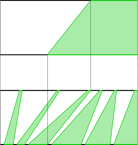
Figure 4. Sketch of the proof of Lemma 3.2 where two different partitions are matched up. The figure represents two iterations of the process in the proof of Lemma 3.2. The lighter intervals, like $I_{\{1,3\}}$, have small capacity in the domain and are mapped to intervals with larger capacity, like $J_{\{1,3\}}=h(I_{\{1,3\}})$. At each step $n$, the maps $h_{n}$ are linear on each $I_{A_{n}}$.

By construction they also satisfy that, if $n\leq m$, then $h_{m}(I_{A_{n}})=J_{A_{n}}$ and $h_{n}(I_{A_{m}})\subset J_{A_{m-1}}$. By hypothesis, given $\varepsilon>0$ there is $N>0$ so that for $n\geq N$ the segments $J_{A_{n}}=h(I_{A_{n}})$ all have length less than $\varepsilon$. Now, if $m\geq n$ and $x\in I$, there exists a word $A_{n}$ so that $x\in I_{A_{n}}$ and $h_{m}(x)\in J_{A_{n}}=h_{n}(I_{A_{n}})$. Hence,

$$|h_{n}(x)-h_{m}(x)|<\varepsilon.$$

Therefore the sequence $\{h_{n}\}$ is uniformly Cauchy and it has a continuous limit $h\colon I\to J$, which preserves orientation.

If $z\not=w$, there are addresses $A_{\infty},\tilde{A}_{\infty}\in\mathcal{A}_{\infty}$ so that $\chi(A_{\infty})=z$ and $\chi(\tilde{A}_{\infty})=w$. Since $z\not=w$, for some $n>1$, there are finite different subwords $A_{n},\tilde{A}_{n}$ satisfying $z\in I_{A_{n}}$ and $w\in I_{\tilde{A}_{n}}$. Therefore $I_{A_{n}}$ and $I_{\tilde{A}_{n}}$ have disjoint interiors and so do $J_{A_{n}}=h(I_{A_{n}})$ and $J_{\tilde{A}_{n}}=h(I_{\tilde{A}_{n}})$. Hence $h(z)\not=h(w)$ and $h$ is an orientation-preserving homeomorphism.

To finish the proof we need to show that the map $h\colon I\to J$ is log-singular. By hypothesis $\operatorname{Cap}(E)=0$ and $\operatorname{Cap}(h(\mathbb{S}^{1}\setminus E))=\operatorname{Cap}(F)=0$, where $E,F$ are given by the Lemma. Therefore $h$ is log-singular. ∎

Remark 3.4.

It can be proved that given any log-singular map $h\colon I\to J$, the log-singular set $E$ can be taken as in Lemma 3.2 (in terms of a suitable partition $\{I_{A_{n}}\}$ of $I$). The proof follows from [Bis07, Lemma 11] and the following observation: if $h\colon I\to J$ is log-singular, then for any closed sub-arc $S\subset I$, the restriction of $h$ to $S$,

$$h_{S}\colon S\to h(S),$$

is also log-singular.

We now prove that there are zero capacity sets as in Lemma 3.2. To do so we define a suitable address that will yield the zero capacity condition. The construction is the same as in [Bis07, Remark 9] and [You18, Proposition 2.3].

Corollary 3.5 (Constructing a log-singular set).

Let $I$ be a subarc of $\mathbb{S}^{1}$ and consider the sequence $\{L_{n}\}$ given by $L_{0}=1$ and $L_{n+1}=2nL_{n}$. Consider words $A_{n}=\{a_{1},a_{2},\ldots,a_{m}\}$ with $0\leq a_{j}<L_{j}$. Then there exists $\{I_{A_{n}}\}$ a partition of $I=I_{0}=I_{A_{0}}$ satisfying that given $\varepsilon>0$, there exists $N\geq 1$ such that for every $n\geq N$, $|I_{A_{n}}|<\varepsilon$, and so that the set

$$E=\bigcap_{n\in\mathbb{N}}\bigcup_{m\geq n}\left(\bigcup_{A_{m}\in\mathcal{A}_{m}}\bigcup_{j=1}^{L_{m+1}/2}I_{A_{m}(2j-1)}\right)$$

has zero capacity. In particular, it is a log-singular set.

Proof.

We can suppose $I=[0,1]$. The goal is to decompose $[0,1]$ in an iterative way by defining a partition $\{I_{A_{n}}\}$ of $[0,1]$ given by addresses $A_{n}$, so that the set $E$ has zero capacity (therefore it satisfies the condition of Lemma 3.2).

Write $I=I_{\{0\}}\cup I_{\{1\}}$, where both $I_{\{0\}}$ and $I_{\{1\}}$ are closed intervals with disjoint interiors with $\operatorname{Cap}(I_{\{1\}})<2^{-1}$.

Suppose that at the $n$-th step, for $n>1$, we have intervals $I_{A_{n}}$, where $A_{n}=\{a_{1},a_{2},\ldots,a_{n}\}$, with $0\leq a_{j}<L_{j}$, is the address of $I_{A_{n}}$. We build the $I_{A_{n+1}}$ in the following way: divide each $I_{A_{n}}$ first into $n$ closed segments with disjoint interiors of equal length. Then divide each of them into two closed segments with disjoint interiors so that the partition $I_{A_{n+1}}$ satisfies:

$$\operatorname{Cap}\left(\bigcup_{A_{n}\in\mathcal{A}_{n}}\bigcup_{j=1}^{nL_{n}}I_{A_{n}(2j-1)}\right)\leq\sum_{A_{n}\in\mathcal{A}_{n}}\sum_{j=1}^{nL_{n}}\operatorname{Cap}\left(I_{A_{n}(2j-1)}\right)<2^{-n-1}.$$

That is, the capacity of the union of all possible $I_{A_{n+1}}$ with

$$A_{n+1}=\{a_{1},\ldots,a_{n},a_{n+1}\},$$

so that $a_{n+1}$ is odd is less than $2^{-n-1}$. This can always be achieved by making the intervals $I_{A_{n}(a)}$ with $a$ odd smaller (and the rest bigger).

By construction, given $\varepsilon>0$ there is $N>0$ so that for $n\geq N$ the segments $I_{A_{n}}$ all have length less than $\varepsilon$. If we take the set $E$ given by the corollary, then by sub-additivity of capacity we have that for any $n\in\mathbb{N}$,

$$\operatorname{Cap}(E)\leq\sum_{n\geq m}2^{-n}.$$

That is, $\operatorname{Cap}(E)=0$ and by Lemma 3.2 $E$ is a log-singular set. ∎

4. Finding regular log-singular sets. Proof of the main theorem

In this section we prove that given a circle homeomorphism $\phi\colon\mathbb{S}^{1}\to\mathbb{S}^{1}$ there is a log-singular set $E\subset\mathbb{S}^{1}$, given by a partition as in the previous section, so that $\operatorname{Cap}(\phi(E))=0$. This is what we prove in Lemma 4.1. Together with Lemma 3.2 it completes the proof of Theorem 1.4.

Lemma 4.1 (Finding regular log-singular sets).

Let $\phi\colon\mathbb{S}^{1}\to\mathbb{S}^{1}$ be an orientation-preserving circle homeomorphism. Then there exists partition $\{I_{A_{n}}\}$ of $\mathbb{S}^{1}$ and a log-singular set

$$E=\bigcap_{n\in\mathbb{N}}\bigcup_{m\geq n}\left(\bigcup_{A_{m}\in\mathcal{A}_{m}}\bigcup_{j=1}^{L_{m+1}/2}I_{A_{m}(2j-1)}\right),$$

so that $\operatorname{Cap}(\phi(E))=0$. Where the sequence $\{L_{n}\}$ associated with $\{A_{n}\}$ satisfies $L_{0}=1$ and $L_{n}$ even for $n\geq 1$.

Proof.

We can suppose $\phi\colon[0,1]\to[0,1]$. The goal is to decompose $[0,1]$ in an iterative way by defining a partition $\{I_{A_{n}}\}$ of $[0,1]$. However, now we need to ensure that the $I_{A_{n}(2j-2)}$ are mapped to intervals with small capacity (as opposed to Lemma 3.2). This is represented in Figure 5.

Write $I=I_{\{0\}}\cup I_{\{1\}}$, where both $I_{\{0\}}$ and $I_{\{1\}}$ are closed intervals with disjoint interiors so that $\operatorname{Cap}(I_{\{1\}})<2^{-1}$. Make $I_{\{1\}}$ smaller (and thus $I_{\{0\}}$ bigger) so that we also have $\operatorname{Cap}(\phi(I_{\{1\}}))=\operatorname{Cap}(J_{\{1\}})<2^{-1}$.

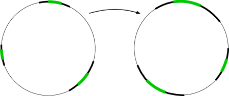
Figure 5. Finding the partition in Lemma 4.1. The lighter thicker sub-arcs have small capacity and they are mapped to sub-arcs with small capacity.

Suppose that at the $n$-th step, for $n>1$, we have intervals $I_{A_{n}}$ and $J_{A_{n}}=h(I_{A_{n}})$, where $A_{n}=\{a_{1},a_{2},\ldots,a_{n}\}$, with $0\leq a_{j}<L_{j}$, is the address of $I_{A_{n}}$, so that

$$\operatorname{Cap}\left(\bigcup_{A_{n-1}\in\mathcal{A}_{n-1}}\bigcup_{j=1}^{L_{n}/2}I_{A_{n-1}(2j-1)}\right)\leq\sum_{A_{n-1}\in\mathcal{A}_{n-1}}\sum_{j=1}^{L_{n}/2}\operatorname{Cap}\left(I_{A_{n-1}(2j-1)}\right)<2^{-n},$$

and their image also has capacity less than $2^{-n}$, i.e.

$$\operatorname{Cap}\left(\bigcup_{A_{n-1}\in\mathcal{A}_{n-1}}\bigcup_{j=1}^{L_{n}/2}J_{A_{n-1}(2j-1)}\right)\leq\sum_{A_{n-1}\in\mathcal{A}_{n-1}}\sum_{j=1}^{L_{n}/2}\operatorname{Cap}\left(J_{A_{n-1}(2j-1)}\right)<2^{-n},$$

We build the $I_{A_{n+1}}$ in the following way: divide each $I_{A_{n}}$ first into $m\geq n$ closed segments with disjoint interior of length less than or equal than $\left(\max_{I_{A_{n}}}|I_{A_{n}}|\right)/n$ so that their images are intervals of length less than or equal than $\left(\max_{J_{A_{n}}}|J_{A_{n}}|\right)/n$. Then divide each of them into two closed segments which yields intervals $I_{A_{n}}$ and $J_{A_{n}}=h(I_{A_{n}})$. By making the $I_{A_{n}(2j-1)}$ smaller we obtain:

$$\operatorname{Cap}\left(\bigcup_{A_{n}\in\mathcal{A}_{n}}\bigcup_{j=1}^{mL_{n}}I_{A_{n}(2j-1)}\right)\leq\sum_{A_{n}\in\mathcal{A}_{n}}\sum_{j=1}^{mL_{n}}\operatorname{Cap}\left(I_{A_{n}(2j-1)}\right)<2^{-n-1},$$

and that their image also has capacity less than $2^{-n-1}$, i.e.

$$\operatorname{Cap}\left(\bigcup_{A_{n}\in\mathcal{A}_{n}}\bigcup_{j=1}^{mL_{n}}J_{A_{n}(2j-1)}\right)\leq\sum_{A_{n}\in\mathcal{A}_{n}}\sum_{j=1}^{mL_{n}}\operatorname{Cap}\left(J_{A_{n}(2j-1)}\right)<2^{-n-1}.$$

If we define $E$ as in the Lemma, then by sub-additivity of capacity we have,

$$\operatorname{Cap}(E)+\operatorname{Cap}(\phi(E))\leq\sum_{n\geq m+1}(2^{-n}+2^{-n})=2^{-m}.$$

Therefore $\operatorname{Cap}(E)=\operatorname{Cap}(\phi(E))=0$. ∎

Remark 4.2.

Observe that the proof of Lemma 4.1 can be modified to obtain a log-singular set $E$ satisfying $\operatorname{Cap}(E)=\operatorname{Cap}(\phi(E))=\operatorname{Cap}(\phi^{-1}(E))=0$.

We finish this section by proving Theorem 1.4.

Proof of Theorem 1.4.

Given $\phi\colon\mathbb{S}^{1}\to\mathbb{S}^{1}$, then by Lemma 4.1 there is a log-singular set $E\subset\mathbb{S}^{1}$ so that $\operatorname{Cap}(\phi(E))=0$. By Lemma 3.2 there exists a log-singular circle homeomorphism $h$ satisfying $\operatorname{Cap}(h(\mathbb{S}^{1}\setminus E))=0$. If we consider the circle homeomorphism $\phi\circ h^{-1}$, then $h(\mathbb{S}^{1}\setminus E)$ has zero capacity and

$$(\phi\circ h^{-1})(\mathbb{S}^{1}\setminus h(\mathbb{S}^{1}\setminus E))=\phi(E),$$

which has zero capacity. Therefore $\phi\circ h^{-1}$ is log-singular. Since log-singular maps are weldings by Theorem 1.3, then

$$\phi=\left(\phi\circ h^{-1}\right)\circ h$$

is a composition of two conformal weldings. ∎

References

- [Ahl06] Lars V. Ahlfors, Lectures on quasiconformal mappings, second ed., University Lecture Series, vol. 38, American Mathematical Society, Providence, RI, 2006, With supplemental chapters by C. J. Earle, I. Kra, M. Shishikura and J. H. Hubbard. MR 2241787
- [AHS23] Morris Ang, Nina Holden, and Xin Sun, The SLE loop via conformal welding of quantum disks, Electronic Journal of Probability 28 (2023), no. none, 1 – 20.
- [AIM09] Kari Astala, Tadeusz Iwaniec, and Gaven Martin, Elliptic partial differential equations and quasiconformal mappings in the plane, Princeton Mathematical Series, vol. 48, Princeton University Press, Princeton, NJ, 2009. MR 2472875
- [AJKS11] Kari Astala, Peter Jones, Antti Kupiainen, and Eero Saksman, Random conformal weldings, Acta Math. 207 (2011), no. 2, 203–254. MR 2892610
- [Bis94] Christopher J. Bishop, Some homeomorphisms of the sphere conformal off a curve, Ann. Acad. Sci. Fenn. Ser. A I Math. 19 (1994), no. 2, 323–338. MR 1274085
- [Bis07] by same author, Conformal welding and Koebe’s theorem, Ann. of Math. (2) 166 (2007), no. 3, 613–656. MR 2373370
- [Bis20] by same author, Conformal removability is hard, Preprint (2020).
- [Car67] Lennart Carleson, Selected problems on exceptional sets, Van Nostrand Mathematical Studies, No. 13, D. Van Nostrand Co., Inc., Princeton, N.J.-Toronto, Ont.-London, 1967. MR 225986
- [DS11] Bertrand Duplantier and Scott Sheffield, Liouville quantum gravity and KPZ, Invent. Math. 185 (2011), no. 2, 333–393. MR 2819163
- [GM08] John B. Garnett and Donald E. Marshall, Harmonic measure, New Mathematical Monographs, vol. 2, Cambridge University Press, Cambridge, 2008, Reprint of the 2005 original. MR 2450237
- [LV60] Olli Lehto and K. I. Virtanen, On the existence of quasiconformal mappings with prescribed complex dilatation, Ann. Acad. Sci. Fenn. Ser. A I 274 (1960), 24. MR 125962
- [LV73] O. Lehto and K. I. Virtanen, Quasiconformal mappings in the plane, second ed., Die Grundlehren der mathematischen Wissenschaften, Band 126, Springer-Verlag, New York-Heidelberg, 1973, Translated from the German by K. W. Lucas. MR 344463
- [Oik61] Kôtaro Oikawa, Welding of polygons and the type of Riemann surfaces, Kodai Math. Sem. Rep. 13 (1961), 37–52. MR 125956
- [Pfl60] Albert Pfluger, Ueber die Konstruktion Riemannscher Flächen durch Verheftung, J. Indian Math. Soc. (N.S.) 24 (1960), 401–412. MR 132827
- [Pom92] Ch. Pommerenke, Boundary behaviour of conformal maps, Grundlehren der mathematischen Wissenschaften [Fundamental Principles of Mathematical Sciences], vol. 299, Springer-Verlag, Berlin, 1992. MR 1217706
- [She16] Scott Sheffield, Conformal weldings of random surfaces: SLE and the quantum gravity zipper, Ann. Probab. 44 (2016), no. 5, 3474–3545. MR 3551203
- [SM06] E. Sharon and D. Mumford, 2d-shape analysis using conformal mapping, International Journal of Computer Vision 70 (2006), no. 1, 55–75.
- [You18] Malik Younsi, Removability and non-injectivity of conformal welding, Ann. Acad. Sci. Fenn. Math. 43 (2018), no. 1, 463–473. MR 3753187