$C^{1}$ robust rigidity for bi-critical circle maps

Abstract.

We prove that two topologically conjugate bi-critical circle maps whose signatures are the same, and whose renormalizations converge together exponentially fast in the $C^{1}$-topology, are $C^{1}$ conjugate.

1. Introduction

In one-dimensional dynamics rigidity occurs when the existence of a weak equivalence between two systems implies the existence of a stronger equivalence between the systems. The general rigidity problem that we are interested in is: when does the existence of a topological conjugacy between two circle maps imply the existence of a smooth conjugacy between these maps?

The study of smoothness of conjugacies between circle maps has been studied at least since the 1960’s. Smooth circle diffeomorphisms are topologically conjugate to a rigid rotation, and the smoothness of this conjugacy is now well understood. Herman [Her79] and Yoccoz [Yoc842] proved that if $f$ is a $C^{r}$ diffeomorphism of the circle, whose rotation number $\rho$ satisfies $|\rho-p/q|\geq C\,q^{-2-\beta}$ for all $p/q\in\mathbb{Q}$, for some $C>0$ and $0\leq\beta<1$, then, provided $r>2\beta+1$, $f$ is $C^{r-1-\beta-\varepsilon}$-conjugate to the corresponding rigid rotation for every $\varepsilon>0$. These results were also proved by Stark [Sta88] and Khanin-Sinai [KS87] using renormalization methods. Later, Khanin and Teplinsky [KT09] showed that the result is also valid for $\varepsilon=0$, provided that $2<r<3$.

Rigidity results have also been shown for classes of circle maps with critical points, in particular for multi-critical circle maps. Multi-critical circle maps are $C^{3}$ maps of the circle with a finite number of non-flat critical points. Any non-flat critical point has an associated real number which is called the criticality of the critical point. Yoccoz proved in [Yoc84] that any multi-critical circle map is topologically conjugate to the corresponding rigid rotation, in particular two multi-critical circle maps with the same irrational rotation number are topologically conjugate to each other. We are interested in studying the smoothness of the conjugacy between two critical circle maps. as opposed to the conjugacy between a critical circle map and the corresponding rigid rotation. If each of the maps only have one critical point and the criticalities of the two critical points are the same then the following smoothness results have been shown for the conjugacy $h$ that sends one critical point to the other: $h$ is quasi-symmetric (and therefore Hölder) [dFdM99]; $h$ is a $C^{1}$ diffeomorphism [KT07, GMdM18] and it is a $C^{1+\alpha}$ diffeomorphism for a full Lebesgue measure subset $\mathcal{A}$ of irrational rotation numbers [dFdM99], provided that the critical maps are $C^{4}$. Moreover, it has been shown [Avi13, dFdM99] that there exist real-analytic and $C^{\infty}$ uni-critical circle maps whose rotation numbers are not contained in $\mathcal{A}$ where the conjugacy is only $C^{1}$ and not $C^{1+\alpha}$.

If the two maps have more that one critical point additional topological invariants appear. Let $f$ be a $C^{3}$ multi-critical circle map with irrational rotation number $\rho$, let $\mu$ be the unique $f-$invariant probability measure (since $f$ is topologically conjugate to an irrational rotation then $f$ is uniquely ergodic), and let $c_{0},\dots,c_{N-1}$ be the non-flat critical points with criticalities $d_{0},\dots,d_{N-1}$ respectively (see Section 2). The signature of the multi-critical circle map $f$ is defined to be the $(2N+2)$-tuple

$$(\rho\,;N;\,d_{0},d_{1},\ldots,d_{N-1};\,\delta_{0},\delta_{1},\ldots,\delta_{N-1}),$$

where $\delta_{i}=\mu[c_{i},c_{i+1})$ (with $c_{N}=c_{0}$).

It is a straight forward to see that if $f$ and $g$ are two $C^{3}$ multi-critical circle maps with the same signature then there is a conjugacy $h$ between them that identifies each critical point of $f$ with one of $g$ and preserves the criticalities. In this paper, we study bi-critical circle maps, these are multi-critical circle maps that have precisely two non-flat critical points. We show the existence of a $C^{1}$ conjugacy between bi-critical circle maps (see Theorem A below) without any restriction on the irrational rotation number. Our main result is the following:

Theorem A.

Let $f$ and $g$ be two $C^{3}$ bi-critical circle maps with the same signature. If the renormalizations of $f$ and $g$ around corresponding critical points converge together exponentially fast in the $C^{1}$ topology, then $f$ and $g$ are $C^{1}$-conjugated.

In [EG23], it was shown (under the same condition on the renormalization as in Theorem A) that two $C^{3}$ bi-critical circle maps are $C^{1+\alpha}$-conjugated if their rotation number belongs to a Lebesgue measure total set $\mathcal{A}$. In particular, those bi-critical circle maps are $C^{1}$-conjugate. Therefore, the main contribution in this paper is to dispose of the hypothesis on the rotation number.

2. Preliminaries

2.1. Multicritical circle maps

A multicritical circle map is an orientation preserving $C^{3}$ circle homeomorphism having $N\geq 1$ non-flat critical points and with irrational rotation number. A critical point $c$ of a $C^{3}$ map $f$ is non-flat of criticality $d>1$ if there exists a neighbourhood $W$ of the critical point such that  $f(x)=f(c)+\phi(x)\,\big{|}\phi(x)\big{|}^{d-1}$ for all $x\in W$, where $\phi:W\rightarrow\phi(W)$ is an orientation preserving $C^{3}$ diffeomorphism satisfying $\phi(c)=0$. As we mentioned in the introduction, any multicritical circle map $f$ has no wandering intervals and in particular it is topologically conjugate with the corresponding rigid rotation [Yoc84].

As an example, we consider a specific case of the generalized Arnold’s family: Let $a\in[0,1)$, $N\in\mathbb{N}$ and let $\tilde{f}_{a}:\mathbb{R}\to\mathbb{R}$ be given by:

$$\tilde{f}_{a}(x)=x+a-\frac{1}{2N\pi}\,\sin(2N\pi x).$$

Each $\tilde{f}_{a}$ is the lift of $f_{a}$, an orientation preserving real-analytic circle homeomorphism, under the universal cover $x\mapsto e^{2\pi ix}$. We can see that each $f_{a}$ is a critical circle map with $N$ cubic critical points, given by $\big{\{}e^{\frac{j}{N}2\pi i}:\,0\leq j\leq N-1\big{\}}$.

2.2. Combinatorics of multicritical circle maps

For an irrational rotation number $\rho\in[0,1)$, let us consider its infinite continued fraction expansion:

$$\rho=[a_{0},a_{1},\cdots]=\cfrac{1}{a_{0}+\cfrac{1}{a_{1}+\cfrac{1}{\ddots}}}\ .$$

Truncating the continued fraction expansion, we obtain the so-called convergents of $\rho$, given by $\frac{p_{n}}{q_{n}}=\;[a_{0},a_{1},\cdots,a_{n-1}].$ The sequence of denominators $\{q_{n}\}_{n\in\mathbb{N}}$ satisfies the following recursive formula:

$$q_{0}=1,\hskip 11.38092ptq_{1}=a_{0},\hskip 11.38092ptq_{n+1}=a_{n}\,q_{n}+q_{n-1}\hskip 8.5359pt\text{for all $n\geq 1$}.$$

Given $f$ a circle homeomorphism with irrational rotation number given by $\rho$ and given any $x\in S^{1}$, the sequence of iterates $\{f^{q_{n}}(x)\}_{n\in\mathbb{N}}$ converges to $x$ (but never coincides with $x$ since we do not have periodic points) alternating the sides where it appoaches. Moreover, the iterate $f^{q_{n}+q_{n+1}}(x)$ is closer to $x$ than $f^{q_{n}}(x)$ but further to $x$ than $f^{q_{n+1}}(x)$. By orientation, $f^{q_{n}+q_{n+1}}(x)$ must be inside the smallest arc that connects $x$ with $f^{q_{n}}(x)$. We denote by $I_{n}(x)$ the interval with endpoints $x$ and $f^{q_{n}}(x)$, which contains the point $f^{q_{n+2}}(x)$. The collection of intervals

$$\mathcal{P}_{n}(x)\ =\ \left\{f^{i}(I_{n}(x)):\;0\leq i\leq q_{n+1}-1\right\}\;\bigcup\;\left\{f^{j}(I_{n+1}(x)):\;0\leq j\leq q_{n}-1\right\}$$

is a partition of the circle (modulo endpoints) called the $n$-th (classical) dynamical partition associated to $x$. The sequence of dynamical partitions $\{\mathcal{P}_{n}(x)\}_{n\in\mathbb{N}}$, for any $x\in S^{1}$, is nested: each element of $\mathcal{P}_{n+1}(x)$ is contained in an element of $\mathcal{P}_{n}(x)$. Those partitions are also refining: the maximal lenght of an element of $\mathcal{P}_{n}(x)$ tends to zero as $n$ tends to infinite. For any $x\in S^{1}$, we denote by $J_{n}(x)$ the union $I_{n}(x)\cup I_{n+1}(x)$ and for any $n\in\mathbb{N}$, we denote by $E_{n}$ the set of endpoints of $\mathcal{P}_{n}(c)$ for $c\in Crit(f)$. With dynamical partitions at hand, we are able to define the renormalization of a critical circle map.

2.3. Renormalization of bi-critical circle maps

We recall the notion of bi-critical commuting pairs, which is a natural generalization of the classical notion of critical commuting pairs.

Definition 2.1.

A $C^{3}$ critical commuting pair with two critical points, also called a bi-critical commuting pair, is a pair $\zeta=(\eta,\xi)$ consisting of two $C^{3}$ orientation preserving homeomorphisms $\xi:I_{\xi}\rightarrow\xi(I_{\xi})$ and $\eta:I_{\eta}\rightarrow\eta(I_{\eta})$, satisfying:

1. $I_{\xi}=[\eta(0),0]$ and $I_{\eta}=[0,\xi(0)]$ are compact intervals in the real line;

2. $(\eta\circ\xi)(0)=(\xi\circ\eta)(0)\neq 0$;

3. $D\xi(x)>0$ for all $x$ and $D\eta(x)>0$ for all $x\neq\beta$;

4. The origin has the same criticality for $\eta$ than for $\xi$;

5. For each $1\leq k\leq 3$, we have that $D^{k}_{-}(\xi\circ\eta)(0)=D^{k}_{+}(\eta\circ\xi)(0)$, where $D_{-}^{k}$ and $D_{+}^{k}$ represent the $k$-th left and right derivative, respectively.

Let $\zeta_{1}=(\eta_{1},\xi_{1})$ and $\zeta_{2}=(\eta_{2},\xi_{2})$ be two $C^{r}$ bi-critical commuting pairs, and let $\tau_{1}:[\eta_{1}(0),\xi_{1}(0)]\rightarrow[-1,1]$ and $\tau_{2}:[\eta_{2}(0),\xi_{2}(0)]\rightarrow[-1,1]$ be the two Mœbius transformations given by

$$\tau_{i}(\eta_{i}(0))=-1,\ \ \tau_{i}(0)=0\ \text{ and }\ \tau_{i}(\xi_{i}(0))=1,$$

for $i\in\{1,2\}$. For all $0\leq r<\infty$ we define the $C^{r}$ pseudo-distance between $\zeta_{1}$ and $\zeta_{2}$ as:

$$d_{r}(\zeta_{1},\zeta_{2})=\max\left\{\left|\dfrac{\xi_{1}(0)}{\eta_{1}(0)}-\dfrac{\xi_{2}(0)}{\eta_{2}(0)}\right|,\ \|\tau_{1}\circ\zeta_{1}\circ\tau_{1}^{-1}-\tau_{2}\circ\zeta_{2}\circ\tau_{2}^{-1}\|_{r}\right\}$$

where $\|\cdot\|_{r}$ represents the $C^{r}$ norm for maps in the interval $[-1,1]$ with a discontinuity at the origin. To get a distance, we restrict to normalized bi-critical commuting pairs: for any given pair $\zeta=(\eta,\xi)$ we denote by $\widetilde{\zeta}$ the pair $(\widetilde{\eta}|_{\widetilde{I_{\eta}}},\widetilde{\xi}|_{\widetilde{I_{\xi}}})$, where tilde means linear rescaling by the factor $1/|I_{\xi}|$. Note that $|\widetilde{I_{\xi}}|=1$ and $|\widetilde{I_{\eta}}|=|I_{\eta}|/|I_{\xi}|$. Equivalently $\widetilde{\eta}(0)=-1$ and $\widetilde{\xi}(0)=|I_{\eta}|/|I_{\xi}|=\xi(0)/\big{|}\eta(0)\big{|}$.

The period of the pair $\zeta=(\eta,\xi)$ is the number $\chi(\zeta)\in\mathbb{N}$ such that $\eta^{\chi(\zeta)}(\xi(0))<0\leq\eta^{\chi(\zeta)-1}(\xi(0)),$ when such number exists. If such number does not exist, i.e. when $\eta$ has a fixed point, we write $\chi(\zeta)=\infty$.

Definition 2.2.

For a pair $\zeta=(\eta,\xi)$ with $\chi(\zeta)<\infty$ and $(\xi\circ\eta)(0)\in I_{\eta}$, we define its pre-renormalization as being the pair

$$p\mathcal{R}(\zeta)=\left(\eta|_{[0,\eta^{\chi(\zeta)}(\xi(0))]}\ ,\ \eta^{\chi(\zeta)}\circ\xi|_{I_{\xi}}\right).$$

Moreover, we define the renormalization of $\zeta$ as the rescaling of $p\mathcal{R}(\zeta)$, that is,

$$\mathcal{R}(\zeta)=\left(\widetilde{\eta}|_{[0,\widetilde{\eta^{\chi(\zeta)}(\xi(0))}]}\ ,\ \widetilde{\eta^{\chi(\zeta)}\circ\xi}|_{\widetilde{I}_{\xi}}\right).$$

If $\zeta$ is a multicritical commuting pair with $\chi(\mathcal{R}^{j}\zeta)<\infty$ for $0\leq j\leq n-1$, we say that $\zeta$ is $n$-times renormalizable, and if $\chi(\mathcal{R}^{j}\zeta)<\infty$ for all $j\in\mathbb{N}$, we say that $\zeta$ is infinitely renormalizable. In the last case, we define the rotation number of the bi-critical commuting pair $\zeta$ as the irrational number whose continued fraction expansion is given by $[\chi(\zeta),\chi(\mathcal{R}\zeta),\cdots,\chi(\mathcal{R}^{n}\zeta),\cdots].$

Let us recall how we obtain a bi-critical commuting pair from a given bi-critical circle map. Let $f$ be a $C^{r}$ bi-critical circle map with $\rho(f)=\rho\in\mathbb{R}\setminus\mathbb{Q}$ and critical points $c_{0},c_{1}$. For a given $c_{i}$, let $\widehat{f}$ be the lift of $f$ (under the universal covering $t\mapsto c_{i}\cdot\exp(2\pi it)$) such that $0<\widehat{f}(0)<1$ (note that $D\widehat{f}(0)=0$). For $n\geq 1$, let $\widehat{I}_{n}(c_{i})$ be the closed interval in $\mathbb{R}$, having the origin as one of its extreme points, which is projected onto $I_{n}(c_{i})$. We define $\xi:\widehat{I}_{n+1}(c_{i})\rightarrow\mathbb{R}$ and $\eta:\widehat{I}_{n}(c_{i})\rightarrow\mathbb{R}$ by $\xi=T^{-p_{n}}\circ\widehat{f}^{q_{n}}$ and $\eta=T^{-p_{n+1}}\circ\widehat{f}^{q_{n+1}}$, where $T(x)=x+1$. Then the pair $(\eta|_{\widehat{I}_{n}(c_{i})},\xi|_{\widehat{I}_{n+1}(c_{i})})$ is a renormalizable bi-critical commuting pair, and its rescaling is denoted by $\mathcal{R}_{i}^{n}f=\left(f^{q_{n+1}}|_{I_{n}(c_{i})},f^{q_{n}}|_{I_{n+1}(c_{i})}\right).$ In other words, let us consider the $n-$th scaling ratio of $f$:

$$s_{n,i}^{f}=\frac{|I_{n+1}(c_{i})|}{|I_{n}(c_{i})|},\ \ \ \ \text{for $i\in\{0,1\}$.}$$

Then the $n-$th renormalization of $f$ at $c_{i}$ is the commuting pair $\mathcal{R}_{i}^{n}f:[-s_{n,i}^{f},1]\to[-s_{n,i}^{f},1]$ given by

$$\mathcal{R}_{i}^{n}f=\begin{dcases}B_{n,f}\circ f^{q_{n}}\circ B_{n,f}^{-1}&\mbox{in $[-s_{n,i}^{f},0)$}\\[4.30554pt] B_{n,f}\circ f^{q_{n+1}}\circ B_{n,f}^{-1}&\mbox{in $[0,1]$,}\\ \end{dcases}$$

where $B_{n,f}$ is the unique orientation-preserving affine diffeomorphism between $J_{n}(c_{i})=I_{n+1}(c_{i})\cup I_{n}(c_{i})$ and $[-s_{n,i}^{f},1]$, that is,

$$B_{n,f}(t)=(-1)^{n}\frac{|t-c_{i}|}{|I_{n}(c_{i})|}.$$

As a straightforward consequence of the combinatorics, we know that $f$ has irrational rotation number if and only if $f$ is infinitely renormalizable. In fact, once we have the $n-$th renormalization of a pair we can obtain the $(n+1)-$th renormalization by iterating $\mathcal{R}_{i}^{n}f(B_{n,f}(1))$ as many times until we observe a change in the signal of the images. By combinatorics that number coincides with $\ a_{n+1}+1$, since

$$(\mathcal{R}_{i}^{n}f)^{a_{n+1}+1}(B_{n,f}(1))<0<(\mathcal{R}_{i}^{n}f)^{a_{n+1}}(B_{n,f}(1)).$$

The $(n+1)-$th renormalization (whose graph before being normalized is represented by the pair of maps inside the small blue box in Figure 1) is

$$\left(B_{n+1,f}\circ f^{q_{n+2}}\circ B_{n+1,f}^{-1}|_{[-1,0]},\ B_{n+1,f}\circ f^{q_{n+1}}\circ B_{n+1,f}^{-1}|_{[0.s_{n+1,i}^{f}]}\right).$$

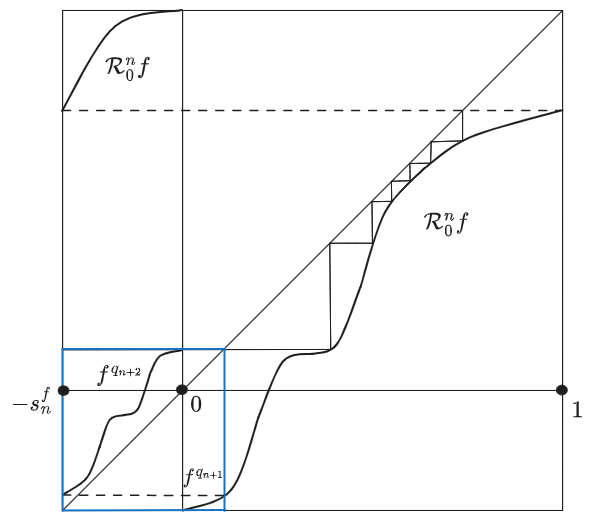
Figure 1. The $n-$th renormalization (in black) and the $(n+1)$-th pre-renormalization (in blue) of a bi-critical circle map $f$ around the critical point $c_{0}$.

Let $f$ and $g$ be two critical circle maps with same signature. We say that their corresponding renormalizations converge together exponentially fast, around the critical point $c_{i}$, in the $C^{r}$-topology if $f$ and $g$ are infinitely renormalizable and there exist $n_{0}\in\mathbb{N}$, $C>0$, $\lambda\in(0,1)$ (both depending on the signature) such that for all $n\geq n_{0}$

$$d_{r}(\mathcal{R}_{i}^{n}f,\mathcal{R}_{i}^{n}g)\leq C\,\lambda^{n}.$$ (1)

In particular, inequality (1) implies that for all $n\geq n_{0}$

$$\left|\frac{|I_{n}(c_{i})|}{|I_{n+1}(c_{i})|}-\frac{|h(I_{n}(c_{i}))|}{|h(I_{n+1}(c_{i}))|}\right|\leq C\,\lambda^{n}.$$

2.4. Real bounds

Now, let us mention a geometric control on the dynamical partitions that implies the pre-compactness of the set $\{\mathcal{R}^{n}f\}_{n\in\mathbb{N}}$ in the $C^{0}$-topology. That geometric control is called real bounds (see [Her88, Swi88] and [EdF18, EdFG18]).

Theorem 2.1 (Universal Real Bounds).

Given $N\in\mathbb{N}$ and $d\in\mathbb{R}$, with $d>1$, let $\mathcal{F}_{d}$ be the family of $C^{3}$ bi-critical circle maps whose maximum criticality is bounded by $d$. There exists $C_{0}=C_{0}(N,d)>1$ such that for any $f\in\mathcal{F}_{d}$ and $c\in\operatorname{Crit}(f)$ there exists $n_{0}\in\mathbb{N}$ with the property that: for all $n\geq n_{0}$ and every adjacent intervals $I,J\in\mathcal{P}_{n}(c)$, we have

$$\frac{1}{C_{0}}\leq\frac{|I|}{|J|}\leq C_{0}\,.$$

In other words, real bounds say that the lenghts of adjacent intervals in the dynamical partition are comparable. Real bounds are also true even if the circle map has not only two but a finite number of critical points (see [EdF18, EdFG18]).

The following result is a consequence of universal real bounds.

Corollary 2.2.

(Exponential refining) There exists a constant $\mu=\mu(C_{0})\in(0,1)$, universal in $\mathcal{F}_{N,d}$, such that for all $m>n\geq n_{0}$: if $\mathcal{P}_{m}(c)\ni I\subseteq J\in\mathcal{P}_{n}(c)$, then $|I|\leq\mu^{m-n}|J|$.

2.5. Two tools: Schwarzian derivative and Koebe Distortion Principle

Recall that for a given $C^{3}$ map $f$ we can define its Schwarzian derivative, which is the differential operator defined (for all $x$ regular point of $f$) by:

$$Sf(x)=\frac{D^{3}f(x)}{Df(x)}-\frac{3}{2}\left(\frac{D^{2}f(x)}{Df(x)}\right)^{2}.$$

For multicritical circle maps we have the following result concerning the Schwarzian derivative:

Lemma 2.3.

[EdFG18, Lemma 4.1] Let $f$ be a multicritical circle map and $c\in\operatorname{Crit}(f)$. There exists $n_{1}=n_{1}(f)\in\mathbb{N}$ such that for all $n\geq n_{1}$ we have that:

$$Sf^{j}(x)<0\text{ \ for all $j\in\{1,\dots,q_{n+1}\}$ and for all $x\in I_{n}(c)$ regular point of $f^{j}$,}$$

and

$$Sf^{j}(x)<0\text{ \ for all $j\in\{1,\dots,q_{n}\}$ and for all $x\in I_{n+1}(c)$ regular point of $f^{j}$.}$$

It is known that the Schwarzian derivative of the composition of two (sufficiently differentiable) functions $f$ and $g$ is given by:

$$S(f\circ g)(z)=\left((Sf)\circ g\right)(z)\cdot(Dg(z))^{2}+Sg(z).$$

Moreover, it is also know that Mobius transformations are the only functions with zero Schwarzian derivative. Hence, the Schwarzian derivative of the renormalization is given by:

$$S(\mathcal{R}_{0}^{n}f)=\begin{dcases}\left((Sf^{q_{n}})\circ B_{n,f}^{-1}\right)\cdot\left(DB_{n,f}^{-1}(z)\right)^{2}&\mbox{in $[-s_{n,0}^{f},0)$}\\[4.30554pt] \left((Sf^{q_{n+1}})\circ B_{n,f}^{-1}\right)\cdot\left(DB_{n,f}^{-1}(z)\right)^{2}&\mbox{in $[0,1]$.}\\ \end{dcases}$$

In particular, $S(\mathcal{R}_{0}^{n}f)(z)<0$ for all $n\geq n_{1}$ and for all $z\in[-s_{n,0}^{f},1]$ regular point.

The Koebe Distortion Principle gives a control on the distortion of high iterates of the map. Recall that given two intervals $M\subset T\subset S^{1}$, with $M\Subset T$, we define the space of $M$ inside $T$ as the smallest of the ratios $|L|/|M|$ and $|R|/|M|$, where $L$ and $R$ denote the two connected components of $T\setminus M$. If the space is $\tau>0$, we say that $T$ contains a $\tau$-scaled neighborhood of $M$. For multicritical circle maps we have the following Koebe Distortion Principle.

Lemma 2.4.

For each $\gamma,\tau>0$ and each multicritical circle map $f$, there exists a constant

$$K=\left(1+\frac{1}{\tau}\right)^{2}\exp(\widetilde{C_{0}}\gamma)\ >1,$$

where $\widetilde{C_{0}}>0$ only depends on $f$, with the following property: if $T$ is an interval such that $f^{k}|_{T}$ is a diffeomorphism onto its image and if $\sum_{j=0}^{k-1}|f^{j}(T)|\leq\gamma$, then for each interval $M\subset T$ for which $f^{k}(T)$ contains a $\tau$-scaled neighborhood of $f^{k}(M)$ we have for all $x,y\in M$

$$\frac{1}{K}\leq\frac{|Df^{k}(x)|}{|Df^{k}(y)|}\leq K.$$

Next result give us a decomposition of the iterates of intervals in the dyamical partition.

Lemma 2.5.

(Decomposition) [EdFG18, Lemma 5.1] Given $\varepsilon>0$ there exists $n_{2}\in\mathbb{N}$, depending on $f$ and $\varepsilon$, with the following property: given $n\geq n_{2}$, $I\in\mathcal{P}_{n}$ and $k\in\mathbb{N}$ for which $f^{j}(I)$ is contained in an element of $\mathcal{P}_{n}$, for all $1\leq j\leq k$, we have the following decomposition:

$$f^{k}(I^{*})=\widehat{\phi}_{k}\circ\widehat{\phi}_{k-1}\circ\dots\circ\widehat{\phi}_{1}$$

where,

1. For at most $7$ values of $i\in\{1,\cdots,k\}$, $\widehat{\phi}_{i}$ is a diffeomorphism with bounded distortion by $1+\varepsilon$.

2. For at most $6$ values of $i\in\{1,\cdots,k\}$, $\widehat{\phi}_{i}$ is the restriction of $f$ to some interval contained in $U_{i}$.

3. For the reminer values of $i$, $\widehat{\phi}_{i}$ is either the identity or a diffeomorphism with negative Schwarzian derivative.

2.6. Controlled bi-critical commuting pairs

Real bounds also give us some control on the lenght of certain intervals, dynamically defined, and some control on the first and second derivatives of the renormalizations.

Definition 2.3.

($M$-controlled bi-critical communting pair) Let $M>1$ and let $\zeta=(\eta,\xi)$ be a normalized $C^{3}$ bi-critical commuting pair, with period $a=\chi(\zeta)\in\mathbb{N}$ and with critical points given by $0$ and $\beta$. We say that $\zeta$ is $M$-controlled if the following conditions are satisfied:

1. $1/M\leq\xi(0)\leq M$;

2. $1/M\leq\xi(0)-\eta(\xi(0))$;

3. $1/M\leq\eta^{a-1}(\xi(0))-\eta^{a}(\xi(0))$;

4. $1/M\leq\eta^{a}(\xi(0))$;

5. $\eta^{a+1}(\xi(0))\leq-1/M$;

6. $\|\xi\|_{C^{2}([\eta(0),0])}\leq M$;

7. $\|\eta\|_{C^{2}([0,\xi(0)])}\leq M$;

8. $1/M\leq D\eta(x)$, for all $x\in[\eta^{a}(\xi(0)),\xi(0)]\setminus\{\beta\}$.

If $\beta\notin(0,\eta^{a+1}(\xi(0)))$ or $\beta\notin(\eta(\xi(0)),\xi(0))$, then the following extra condition is also satisfied:

1. $\eta(\beta)-\beta\geq 1/M$ and $\beta-\eta^{-1}(\beta)\geq 1/M$.

Next result guarantes that every $C^{3}$ bi-critical circle map with irrational rotation number gives rise to a sequence of bi-critical controlled commuting pairs, after a finite number of renormalizations.

Theorem 2.6.

There exists a universal constant $M>1$ with the following property. For any given $C^{3}$ bi-critical circle map $f$ with irrational rotation number there exists $n_{0}=n_{0}(f)\in\mathbb{N}$ such that the critical commuting pair $\mathcal{R}^{n}f$ is $M$-controlled for any $n\geq n_{0}$.

Proof of Theorem 2.6.

By universal real bounds (Theorem 2.1), there exists a constant $C>1$ and $n_{0}\in\mathbb{N}$ such that for any $n\geq n_{0}$ properties $(1)$ to $(5)$ and property $(8)$ hold. Moreover, by [EdF18, Lemma 4.2, Lemma 4.1] and real bounds we know that $\left|[\eta(\beta),\beta]\right|$ is comparable with $\xi(0)$, then by Property $(1)$ $|\eta(\beta)-\beta|\geq 1/M$. By [EdF18, Lemma 3.3], $\left|\beta-\eta^{-1}(\beta)\right|\geq 1/M$, and hence property $(9)$ is also true. Finally, from [EdFG18, Lemma 5.1] and [dFdM99, Lemma A.4], there exists $n_{0}\in\mathbb{N}$ such that for all $n\geq n_{0}$ properties $(6)$ and $(7)$ hold. ∎

Remark 2.1.

By [dFdM99, Lemma A4], the renormalizations of a $C^{3}$ uni-critical circle map are controlled as in our definition. That result and its proof can be generalized to the bi-critical case.

3. The two-bridges partition $\widehat{\mathcal{P}}_{n}$

In this section we recall the construct of the sequence of two-bridges partitions $\{\widehat{\mathcal{P}}_{n}\}_{n\in\mathbb{N}}$, defined in [EG23, Section 4.1.1]. Let $c_{0}$ and $c_{1}$ be the two critical points of $f$. For $n\in\mathbb{N}$, the first return map to $J_{n}(c_{0})$, which is given by $(f^{q_{n+1}}|_{I_{n}(c_{0})},f^{q_{n}}|_{I_{n+1}(c_{0})})$, has two critical points: one being $c_{0}$ and the other one being the unique preimage of $c_{1}$ for the return. Such preimage in $J_{n}(c_{0})$ is called the free critical point at level $n$, and is denoted by $\mathfrak{c}_{n,0}$. Without lost of generality, let us assume that $\mathfrak{c}_{n,0}$ belongs to $I_{n}(c_{0})$. This means that there exists $j<q_{n+1}$ such that $c_{1}\in f^{j}(I_{n}(c_{0}))$ and $f^{j}(\mathfrak{c}_{n,0})=c_{1}$. Note that if $c_{1}$ belongs to the positive orbit of $c_{0}$ then there exists $m\in\mathbb{N}$ such that for all $n\geq m$ the return maps $(f^{q_{n+1}}|_{I_{n}(c_{0})},f^{q_{n}}|_{I_{n+1}(c_{0})})$ are unicritical and we will be in the situation studied in [KT07]. So, from now on, let us assume that $c_{1}$ does not belong to the positive orbit of $c_{0}$. Moreover we will assume that $n\geq n_{0}$ where $n_{0}$ is given by Theorem 2.6.

Definition 3.1 (Two-bridges level).

A natural number $n$ is a two-bridges level for $f$ at $c_{0}$ if $a_{n+1}\geq 23$, the free critical point $\mathfrak{c}_{n}$ belongs to $I_{n}(c_{0})\setminus I_{n+2}(c_{0})$ and moreover $\mathfrak{c}_{n}\in\{\Delta_{11},\Delta_{12},\dots,\Delta_{a_{n+1}-10}\}$, where $\Delta_{j}=f^{(j-1)q_{n+1}+q_{n}}(I_{n+1}(c_{0}))$ for all $j\in\{1,\dots,a_{n+1}\}$.

We recall the inductive construction of the two-bridges partition $\widehat{\mathcal{P}}_{n}$ for $n\geq 0$. To start we define $\widehat{\mathcal{P}}_{0}$ be the same as $\mathcal{P}_{0}$, now for $n\in\mathbb{N}$ we have two cases:

Case 1: $n$ is a two-bridges level for $f$ at $c_{0}$. Then we consider the following six pairwise disjoint intervals in $I_{n}(c_{0})\setminus I_{n+2}(c_{0})$:

$$\Delta_{1}=f^{q_{n}}(I_{n+1}(c_{0})),\ \ \widehat{\Delta}_{n}=[f^{q_{n+1}}(\mathfrak{c}_{n}),\mathfrak{c}_{n}]$$

$$\Delta_{a_{n+1}}=f^{(a_{n+1}-1)q_{n+1}}(\Delta_{1})=[f^{q_{n+2}}(c_{0}),f^{(a_{n+1}-1)q_{n+1}+q_{n}}(c_{0})].$$

For each $j\in\mathbb{Z}$, denote by $\Delta_{1}^{j}$, $\widehat{\Delta}_{n}^{j}$ and $\Delta_{a_{n+1}}^{j}$ the intervals $f^{jq_{n+1}}(\Delta_{1})$, $f^{jq_{n+1}}(\widehat{\Delta}_{n})$ and $f^{jq_{n+1}}(\Delta^{a_{n+1}})$, respectively. Let $r(n),\ell(n)\in\{0,\dots,a_{n+1}\}$ be given by

$$r(n)=\min\{j\in\mathbb{N}:\widehat{\Delta}_{n}^{-j}\cap\Delta_{1}^{j}\neq\emptyset\}\text{ \ and \ }\ell(n)=\min\{j\in\mathbb{N}:\Delta_{a_{n+1}}^{-j}\cap\widehat{\Delta}_{n}^{j}\neq\emptyset\}.$$

Note that the intersections above may be given by a single point (in this case the critical points have the same orbit). Just to fix ideas, let us assume that $\Delta_{a_{n+1}}^{-\ell(n)}\setminus\widehat{\Delta}_{n}^{\ell(n)}\subset\widehat{\Delta}_{n}^{\ell(n)+1}$  and  $\widehat{\Delta}_{n}^{-r(n)}\setminus\Delta_{1}^{r(n)}\subset\Delta_{1}^{r(n)+1}$, we consider $\Delta_{R}^{n+1}=\Delta_{1}^{r(n)}\cup\widehat{\Delta}_{n}^{-r(n)}$ and $\Delta_{L}^{n+1}=\Delta_{a_{n+1}}^{-\ell(n)}\cup\widehat{\Delta}_{n}^{\ell(n)}$. We define $\widehat{\mathcal{P}}_{n+1}$ inside $I_{n}(c_{0})$, for a two-bridges level $n$, as

$$\widehat{\mathcal{P}}_{n+1}|_{I_{n}(c_{0})}=\{I_{n+2}(c_{0}),\{\Delta_{a_{n+1}}^{-j}\}_{j=0}^{j=\ell(n)-1},\Delta_{L}^{n+1},\{\widehat{\Delta}_{n}^{j}\}_{j=1-r(n)}^{j=\ell(n)-1},\Delta_{R}^{n+1},\{\Delta_{1}^{j}\}_{j=0}^{j=r(n)-1}\}.$$

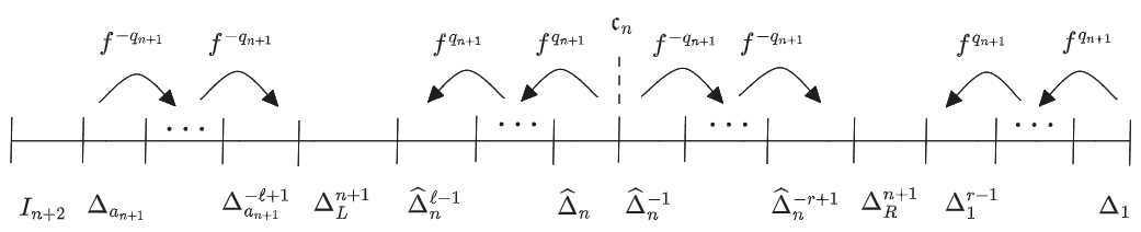
Figure 2. The two-bridges partition $\widehat{\mathcal{P}}_{n+1}|_{I_{n}(c_{0})}$ in Case 1.

Now, we spread the definition of $\widehat{\mathcal{P}}_{n+1}$ to the circle as usual, that is:

$$\widehat{\mathcal{P}}_{n+1}=\{f^{i}(I_{n+1}(c_{0})):0\leq i\leq q_{n}-1\}\ \bigcup\ \{f^{j}(I)|_{I\in\widehat{\mathcal{P}}_{n+1}\cap I_{n}(c_{0})}:0\leq j\leq q_{n+1}-1\}.$$

Case 2: $n$ is not a two-bridges level for $f$ at $c_{0}$, then $\widehat{\mathcal{P}}_{n+1}$ coincides with $\mathcal{P}_{n+1}$ except in the following cases. For any given endpoint $v$ of $\widehat{\mathcal{P}}_{n}$, let $I^{\prime}\in\mathcal{P}_{n+1}$ be the interval containing $v$ and let $w$ be the endpoint of $I^{\prime}$ closest to $v$ (in the Euclidean distance).

• If $v$ is the middle point of $I^{\prime}$, then we add $v$ to the set of endpoints of $\widehat{\mathcal{P}}_{n+1}$.

• If $v$ is not the middle point of $I^{\prime}$: we remove $w$ from the set of endpoints of $\widehat{\mathcal{P}}_{n+1}$ and we add $v$ to the set of endpoints of the partition $\widehat{\mathcal{P}}_{n+1}$.

3.1. Properties of the two-bridges partition

For any $n\in\mathbb{N}$ we denote by $\widehat{E}_{n}$ the set of the endpoints of $\widehat{\mathcal{P}}_{n}$. We observe that, from the construction, when we lost one endpoint of $E_{k}$ by defining $\widehat{E}_{k}$, that missing endpoint will appear in the next level, that is in $\widehat{E}_{k+1}$. From the construction we have the following properties of $\{\widehat{\mathcal{P}}_{n}\}_{n\in\mathbb{N}}$:

1. Each partition $\widehat{\mathcal{P}}_{n}$ is dynamically defined: each $v\in\widehat{E}_{n}$ is an iterate (either forward or backward) of a first return map at $c_{0}$ or $c_{1}$.

2. The intervals $I_{n}(c_{0})$ and $I_{n+1}(c_{0})$ belong to $\widehat{\mathcal{P}}_{n+1}$.

3. The sequence of partitions $\{\widehat{\mathcal{P}}_{n}\}$ is nested.

4. The sequence of partitions $\{\widehat{\mathcal{P}}_{n}\}$ is refining.

5. If $n$ is a two-bridges level for $f$ at $c_{0}$ then $\mathfrak{c}_{n}\in\widehat{E}_{n+1}$.

6. Any endpoint of the standard partition $\mathcal{P}_{n}$ belongs to $\widehat{E}_{m}$ for some $m\geq n$.

7. (Real bounds) There exists an universal constant $\widehat{C}>1$, such that $\widehat{C}^{-1}|I|\leq|J|\leq\widehat{C}|I|$ for each pair of adjacent atoms $I,J\in\widehat{\mathcal{P}}_{n}$.

Corollary 3.1.

(Exponential refining) There exist a constant $\widehat{\mu}\in(0,1)$ and $n_{0}\in\mathbb{N}$, both universal in $\mathcal{F}_{2,d}$, such that for all $m>n\geq n_{0}$: if $\widehat{\mathcal{P}}_{m}\ni I\subseteq J\in\widehat{\mathcal{P}}_{n}$, then $|I|\leq\widehat{\mu}^{m-n}|J|$.

For different levels of the two-bridges partition, we have

Lemma 3.2.

[EG23, Lemma 4.6] Let $n,p\in\mathbb{N}$, and $v$ be an endpoint of $\widehat{\mathcal{P}}_{n+p}$ contained in $J_{n}(c_{0})$. There exist $L\in\{1,...,p\}$ and $n\leq m_{1}\leq\dots\leq m_{L}$, such that $v=\phi_{1}\circ\dots\circ\phi_{L}(x)$, where

1. For each $j\in\{1,\dots,L\}$ we have $\phi_{j}=f^{k_{j}q_{m_{j}+1}+\sigma_{j}q_{m_{j}}}$ for $\sigma_{j}\in\{0,1\}$ and $k_{j}\in\mathbb{Z}$ either satisfying $|k_{j}|\leq\ell(m_{j})$ and $|k_{j}|\leq r(m_{j})$ or $|k_{j}|\leq\lceil a_{m_{j}+1}/2\rceil$, depending on whether $m_{j}$ is or is not a two-bridges level for f at $c_{0}$.

2. For each $j\in\{1,\dots,L-1\}$, the point $\phi_{j+1}\circ\dots\circ\phi_{L}(x)$ either belongs to $J_{m_{j}+1}(c_{0})\cup\widehat{\Delta}_{m_{j}}$ or to $J_{m_{j}+1}(c_{0})$, depending on whether $m_{j}$ is or is not a two-bridges level.

3. There exists $m\in\{m_{L},\dots,n+p\}$, such that $x$ belongs to $\{c_{0},f^{q_{m+2}}(c_{0}),\mathfrak{c}_{m}\}$ or to $\{c_{0},f^{q_{m+2}}(c_{0})\}$, depending on whether $m$ is or is not a two-bridges level.

Remark 3.1.

The relation between the lenght of interval is the classical dynamical partition and the two-bridges partition is the following: let $C>1$ and $\widehat{C}>1$ be the two constants given by real bounds of the classical and the two-bridges partition, respectively. If $I\in\mathcal{P}_{n}$ and $\widehat{I}\in\widehat{\mathcal{P}}_{n}$ and $I\cap\widehat{I}\neq\emptyset$ then

$$\frac{1}{\max\{C+1,\widehat{C}+1\}}\leq\frac{|I|}{|\widehat{I}|}\leq\max\{C+1,\widehat{C}+1\}.$$

4. Idea of the proof

The proof of our Main Theorem consists in to construct a sequence of circle partitions that satisfy some especific properties. More precisely, we want to prove the following result:

Proposition 4.1.

[KT07, Proposition, Page 199] Let $h$ be a circle map and $\{\mathcal{Q}_{n}^{f}\}_{n\in\mathbb{N}}$ and $\{\mathcal{Q}_{n}^{g}\}_{n\in\mathbb{N}}$ be two sequences of circle partitions such that for all $I\in\mathcal{Q}_{n}^{f}$ we have $h(I)\in\mathcal{Q}_{n}^{g}$. Suppose also that:

1. $\{\mathcal{Q}_{n}^{f}\}_{n\in\mathbb{N}}$ and $\{\mathcal{Q}_{n}^{g}\}_{n\in\mathbb{N}}$ are sequence of refinement circle partitions;

2. the maximal lenght of an interval in $\mathcal{Q}_{n}^{f}$, and the maximal lenght of an interval in $\mathcal{Q}_{n}^{g}$, go to zero as $n$ goes to infinite;

3. there exist $B>0$ and $\mu\in(0,1)$ such that for any two intervals $I,I^{\prime}\in\mathcal{Q}_{n}^{f}$, which either are adjacent or $I,I^{\prime}\subset J$ for some $J\in\mathcal{Q}_{n-1}^{f}$, we have

   $$\left|\log\frac{|h(I)|}{|I|}-\log\frac{|h(I^{\prime})|}{|I^{\prime}|}\right|\leq B\,\mu^{n};$$

then $h$ is a $C^{1}$ circle diffeomorphism.

We will prove that the sequence of two-bridges partition $\{\mathcal{\widehat{P}}_{n}^{f}\}_{n\in\mathbb{N}}$, and its corresponding sequence $\{\mathcal{\widehat{P}}_{n}^{g}\}_{n\in\mathbb{N}}$ for $n\geq n_{0}$ where $n_{0}$ is given by Theorem 2.6, satisfy the three conditions in Proposition 4.1. The only condition that is not a consequence of the definition and properties of $\{\mathcal{\widehat{P}}_{n}^{f}\}_{n\in\mathbb{N}}$ is the third one, our main aim in this paper is to prove condition $(3)$ in Proposition 4.1.

Let us add some words about how we will obtain condition $(3)$:

1. First, we fixed $m\in\mathbb{N}$, and we the consider the two fundamental domain of the renormalizations $J_{m}(c_{0})$ and $J_{m}(c_{1})$. Inspired by [KT07], in Section 5 we prove that there exists an uniform strip around $m$ where, for all $n$ in that strip, the distance between each endpoint in $\widehat{E}_{n}$ (contained in $J_{m}(c_{0})$ or in $J_{m}(c_{1})$) and its image by $h$ is exponentially small, at rate $n$. We get those estimates in Proposition 6.1.

2. Second, using the step before and the shape of the renormalizations inside $J_{m}(c_{0})$ and $J_{m}(c_{1})$, we get inequality $(3)$ in Proposition 4.1 for intervals in $\mathcal{\widehat{P}}_{n}^{f}$ which are contained in $J_{m}(c_{0})\cup J_{m}(c_{1})$. Those estimates are proved in Proposition 7.3.

3. Finally, using Koebe Distortion Principle (Lemma 2.4) and the fact that we can take any pair of intervals of $\mathcal{\widehat{P}}_{n}^{f}$ inside $J_{m}(c_{0})$ or $J_{m}(c_{1})$, by a diffeomorphism, we extend the estimates obtained in second step to intervals outside $J_{m}(c_{0})\cup J_{m}(c_{1})$.

To obtain the proof of step 1 (Section 6), we need some background given in Section 5. The proof of step 2 is given in Section 7. The final step will be proved in Section 8.

5. Un-bounded rotation number

From now on, for all $n\in\mathbb{N}$, we will renormalize around $c_{0}$, so we write $I_{n}^{f}$, $I_{n+1}^{f}$, $J_{n}^{f}$, $\mathfrak{c}_{n}$, $s_{n}^{f}$ and $\mathcal{R}^{n}f$ instead of $I_{n}^{f}(c_{0})$, $I_{n+1}^{f}(c_{0})$, $J_{n}^{f}(c_{0})$, $\mathfrak{c}_{n,0}^{f}$, $s_{n,0}^{f}$ and $\mathcal{R}_{0}^{n}f$ respectively. Since $h$ is the conjugacy that identifies corresponding critical points, then $\mathfrak{c}_{n}^{g}=h(\mathfrak{c}_{n})$. We notice that the construction, definitions and results given in this section can be extended if we renormalize around $c_{1}$.

We say that an irrational number $\rho=[a_{0},a_{1},\dots,a_{n},\dots]\in[0,1)$ is bounded type if there exists $A\in\mathbb{N}$ such that $\sup_{k}a_{k}\leq A$. The set of bounded type rotation numbers has zero Lebesgue measure in $[0,1]$. As we mentioned in the introduction, we focus our attention on un-bounded type rotation numbers, i.e. $\rho=[a_{0},a_{1},\cdots,a_{n},\cdots]$ such that there is no $A\in\mathbb{N}$ such that $\sup_{k}a_{k}<A$. In particular, the fundamental interval $I_{k}$ is subdivided by an un-bounded number of subintervals of the classical dynamical partition $\mathcal{P}_{k+1}$, and hence the graph of $\mathcal{R}^{k}f$ is arbitrarily close to the identity.

For a given $n\in\mathbb{N}$ and $L\in\mathbb{N}$, we define the $L-$th tubular of $\mathcal{R}^{n}f$ as the set:

$$M_{n,L}^{f}=\{z\in[0,1]:z-\mathcal{R}^{n}f(z)<1/L\}.$$

We observe that if $a_{n+1}>L$ then the set $M_{n,L}^{f}$ is not empty.

Lemma 5.1.

Given $M>1$ such that $\mathcal{R}^{n}f$ is $M$-controlled, there exists $L=L(M)\in\mathbb{N}$ such that:

1. $r(n)\geq L$, and in this case there exists an unique point $p\in Int[(\mathcal{R}^{n}f)^{-1}(B_{n,f}(\mathfrak{c}_{n})),1]$ such that $|\mathcal{R}^{n}f(p)-p|\leq|\mathcal{R}^{n}f(z)-z|$ for all $z\in[(\mathcal{R}^{n}f)^{-1}(B_{n,f}(\mathfrak{c}_{n})),1]$, $D\mathcal{R}^{n}f(p)=1$ and $D^{2}\mathcal{R}^{n}f(p)<0$.

2. If $\ell(n)\geq L$ then there exists an unique point $q\in Int[0,\mathcal{R}^{n}f(B_{n,f}(\mathfrak{c}_{n}))]$ such that $|\mathcal{R}^{n}f(q)-q|\leq|\mathcal{R}^{n}f(z)-z|$ for all $z\in[0,\mathcal{R}^{n}f(B_{n,f}(\mathfrak{c}_{n}))]$, $D\mathcal{R}^{n}f(q)=1$ and $D^{2}\mathcal{R}^{n}f(q)<0$.

Proof.

Note that $S(\mathcal{R}^{n}f)<0$ in $[0,\mathcal{R}^{n}f(B_{n,f}(\mathfrak{c}_{n}))]\cup[(\mathcal{R}^{n}f)^{-1}(B_{n,f}(\mathfrak{c}_{n})),1]$. The proof follows from a small adaptation of the proof of [GMdM18, Lemma 6.1]. ∎

By Lemma 5.1 and [GMdM18, Remark 6.2]

Corollary 5.2.

Given $M>1$ there exists $L=L(M)\in\mathbb{N}$ such that $M_{n,L}^{f}$ is a non empty open interval, which can be an open interval or two open intervals, that contains at most two points $z_{n}^{f}$ and $w_{n}^{f}$ which attains the minimum of $|z-\mathcal{R}^{n}f(z)|$ inside $M_{n,L}^{f}$. For those points we have $D\mathcal{R}^{n}f(z_{n}^{f})=1$, $D\mathcal{R}^{n}f(w_{n}^{f})=1$, $D^{2}\mathcal{R}^{n}f(z_{n}^{f})<-1/M$ and $D^{2}\mathcal{R}^{n}f(w_{n}^{f})<-1/M$.

If the points $z_{n}^{f}$ and $w_{n}^{f}$ in Corollary 5.2 exist, then they are called the centers of $M_{n,L}^{f}$. The exponential convergence of the renormalizations, in the $C^{1}$-topology, implies that

$$\left|z_{n}^{g}-z_{n}^{f}\right|=\left|h(z_{n}^{f})-z_{n}^{f}\right|\leq C\,\lambda^{n}$$ (2)

and

$$\left|w_{n}^{g}-w_{n}^{f}\right|=\left|h(w_{n}^{f})-w_{n}^{f}\right|\leq C\,\lambda^{n},$$ (3)

where $h(z_{n}^{f})$ and $h(w_{n}^{f})$ are the centers of $M_{n,L}^{g}$. From now on we denote the centers $z_{n}^{f}$ and $w_{n}^{f}$ by $z_{n}$ and $w_{n}$, respectively.

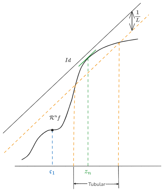
Figure 3. In this figure $r(n)>L$ and then the center $z_{n}$ of $M_{n,L}^{f}$ is defined

5.1. Tubular coordinates

Let us fix $m\in\mathbb{N}$ and $L=L(a_{m+1})\in(0,1)$ such that $M_{m,L}^{f}$ is not empty and the center $z_{m}$ is defined. A similar construction can be done if $w_{m}$ is defined.

Definition 5.1.

The tubular-coordinates of $\mathcal{R}^{m}f$ with respect to $z_{m}$, is defined as the change of coordinates of $\mathcal{R}^{m}f$ given by:

$$\mathcal{F}_{m}(x)=\phi_{m}\circ\mathcal{R}^{m}f\circ\phi_{m}^{-1}(x),$$

where $\phi_{m}(x)=(D^{2}\mathcal{R}^{m}f)(z_{m})(x-z_{m})/2$,  for $x\in[B_{m,f}(f^{-q_{m+1}}(\mathfrak{c}_{m})),B_{m,f}(f^{q_{m}}(c_{0}))]$.

Analogously, we define the tubular-coordinates of $\mathcal{R}^{m}g$ with respect to $h(z_{m})$, as the change of coordinates given by

$$\mathcal{G}_{m}(x)=\psi_{m}\circ\mathcal{R}^{m}g\circ\psi_{m}^{-1}(x),$$

where $\psi_{m}(x)=(D^{2}\mathcal{R}^{m}g)(h(z_{m}))(x-h(z_{m}))/2$,  for $x\in[B_{m,g}(g^{-q_{m+1}}(h(\mathfrak{c}_{m}))),B_{m,g}(g^{q_{m}}(h(c_{0})))]$.

Since a change of coordinates does not affect the original exponential convergence (see e.g. [EG23, Lemma 3.1]), then the exponential convergence of $\mathcal{R}^{m}f$ and $\mathcal{R}^{m}g$ in the $C^{1}$-topology, implies that the tubular-coordinates of $\mathcal{F}_{m}$ and $\mathcal{G}_{m}$ also converge exponentially in the same topology.

We are interested in obtain asymptotics estimates of $\mathcal{F}_{m}$ and of $\mathcal{G}_{m}$, near the origin. Since $\mathcal{F}_{m}^{\prime}(0)=1$, $\mathcal{F}_{m}^{\prime\prime}(0)=2$ and $\varepsilon_{m}=\mathcal{F}_{m}(0)=\min_{x}\{\mathcal{F}_{m}(x)-x\}<0$, then there exists $\mathfrak{C}>0$ such that

$$|\mathcal{F}_{m}(x)-(\varepsilon_{m}+x+x^{2})|\leq\mathfrak{C}|x|^{2+\alpha}\text{, \ for $x\in\phi_{m}([0,1])$ }.$$ (4)

Note that if $|x|^{2+\alpha}>C_{0}\,|\varepsilon_{m}|$, for some $C_{0}>0$, then from (4) we get $|\mathcal{F}_{m}(x)-(x+x^{2})|\leq\widetilde{C}_{0}|x|^{2+\alpha}$, so we can dispose of the value $|\varepsilon_{m}|$. For those points we use the following estimates (see [KT07, Lemma 5]).

Lemma 5.3 (Estimates inside the Funnel).

Let $\{s_{i}\}_{i\geq 0}$ be a sequence of real numbers such that there exist $\widehat{C_{0}}>0$ with $|s_{i+1}-(s_{i}-s_{i}^{2})|\leq\widehat{C_{0}}\,|s_{i}|^{2+\alpha}$ for every $i\geq 0$. Then there exist positive constants $D_{1}$, $D_{2}$ and $d_{1}\in(0,1)$ (all depending on $\widehat{C_{0}}~$ and $\alpha$) such that as long as $s_{0}\in(0,d_{1}]$, then for all $i\geq 0$ we have

$$\left|s_{i}-\frac{1}{i+s_{0}^{-1}}\right|\leq\frac{D_{1}}{(i+s_{0}^{-1})^{1+\alpha}}$$ (5)

and

$$s_{i}-s_{i+1}=\frac{1+\delta_{i}}{(i+s_{0}^{-1})^{2}},\text{ \ for $|\delta_{i}|\leq D_{2}s_{0}^{\alpha}$}.$$ (6)

On the other hand, if $|x|^{2+\alpha}<C_{0}\,\varepsilon_{m}$, for some $C_{0}>0$, then for those points we can use the following estimates (see [KT07, Lemma 6]).

Lemma 5.4 (Estimates inside the Tunnel).

Let $\{s_{i}\}_{i\geq 0}$ be a sequence of real numbers such that there exist $\widetilde{C_{1}},\widetilde{C_{2}}>0$ and $\varepsilon\in(0,1)$ with

1. $|s_{0}|\leq\widetilde{C_{1}}\,\varepsilon$,

2. $|s_{i+1}-(\varepsilon+s_{i}+s_{i}^{2})|\leq\widetilde{C_{2}}|s_{i}|^{2+\alpha}$, for all $i\geq 0$.

Fix arbitrary $\widetilde{C_{3}}>0$ and define $N=N(\widetilde{C_{3}},\varepsilon)=\varepsilon^{-1/2}\,tan^{-1}(\widetilde{C_{3}}\varepsilon^{-\alpha/2(2+\alpha)})$. Then there exist positive constants $D_{3},D_{4}$ and $d_{2}\in(0,1)$ (all depending on $\widetilde{C_{1}},\widetilde{C_{2}},\widetilde{C_{3}}$ and $\alpha$) such that, as long as $\varepsilon\in(0,d_{2}]$, for every $0\leq i\leq N$:

$$\left|s_{i}-\sqrt{\varepsilon}\tan\left(\sqrt{\varepsilon}i+\tan^{-1}\left(\frac{s_{0}}{\sqrt{\varepsilon}}\right)\right)\right|\leq D_{3}(\sqrt{\varepsilon}\tan\sqrt{\varepsilon}i)^{1+\frac{\alpha(\alpha+1)}{2}}$$ (7)

and

$$s_{i+1}-s_{i}=\frac{\varepsilon(1+\delta_{i})}{(\cos\sqrt{\varepsilon}i)^{2}},\text{ \ \ \ where $|\delta_{i}|\leq D_{4}\varepsilon^{\frac{\alpha(\alpha+1)}{2(2+\alpha)}}$ .}$$ (8)

The proofs of Lemma 5.3 and Lemma 5.4 can be found in [KT07, Appendix].

Let us give some more know estimates. First, let $i_{c},\widehat{i_{c}}\in\mathbb{N}$ the smallest natural number such that $\mathcal{F}_{m}^{i_{c}}(\phi_{m}(1))\in(0,-\varepsilon_{m}]$ and $\mathcal{F}_{m}^{-\widehat{i_{c}}}(\phi_{m}(B_{m,f}(\mathfrak{c}_{m})))\in(0,-\varepsilon_{m}]$, respectively. Moreover, let $i_{r},i_{\ell}\in\mathbb{N}$ be such that $\mathcal{F}_{m}^{i_{r}}(\phi_{m}(1))$ is the most right endpoint of the Funnel and $\mathcal{F}_{m}^{i_{\ell}}(\phi_{m}(1))$ is the most left endpoint of the Funnel. Similarly, let $\widehat{i_{r}},\widehat{i_{\ell}}\in\mathbb{N}$ such that $\mathcal{F}_{m}^{-\widehat{i_{\ell}}}(\phi_{m}(B_{m,f}(\mathfrak{c}_{m})))$ is the most left endpoint of the Funnel and $\mathcal{F}_{m}^{-\widehat{i_{r}}}(\phi_{m}(B_{m,f}(\mathfrak{c}_{m})))$ is the most right endpoint of the Funnel.
Analogously, let us define $\sigma_{m}=\mathcal{G}_{m}(0)=\min_{x}\{\mathcal{G}_{m}(x)-x\}<0$. Let $j_{c},\widehat{j_{c}}\in\mathbb{N}$ be the smallest natural numbers such that $\mathcal{G}_{m}^{j_{c}}(\psi_{m}(1))\in(0,-\sigma_{m}]$ and $\mathcal{G}_{m}^{-\widehat{j_{c}}}(\psi_{m}(B_{m,f}(\mathfrak{c}_{m})))\in(0,-\sigma_{m}]$, respectively. Moreover, let $j_{r},j_{\ell}\in\mathbb{N}$ be such that $\mathcal{G}_{m}^{j_{r}}(\psi_{m}(1))$ is the most right endpoint of the Funnel and $\mathcal{G}_{m}^{j_{\ell}}(\psi_{m}(1))$ is the most left endpoint of the Funnel. Similarly, let $\widehat{j_{r}},\widehat{j_{\ell}}\in\mathbb{N}$ such that $\mathcal{G}_{m}^{-\widehat{j_{\ell}}}(\psi_{m}(B_{m,g}(h(\mathfrak{c}_{m}))))$ is the most left endpoint of the Funnel and $\mathcal{G}_{m}^{-\widehat{j_{r}}}(\psi_{m}(B_{m,g}(h(\mathfrak{c}_{m}))))$ is the most right endpoint of the Funnel.

Note that $i_{\kappa}\neq j_{\kappa}$ for $\kappa\in\{c,r,\ell\}$. Next result follows from [KT07, Pages 206-207].

Lemma 5.5.

There exists constants $D_{5}$ and $D_{6}$ such that if $r(m)\geq D_{6}$ then

$$|2r(m)-\pi\varepsilon_{m}^{-1/2}|\leq D_{5}\,\varepsilon_{m}^{\frac{-1+\alpha}{2}}$$

$$\left|\frac{h(\varepsilon_{m})}{\varepsilon_{m}}-1\right|\leq D_{5}\,\varepsilon_{m}^{\alpha/2}$$

$$|i_{c}-r(m)|\leq D_{5}\,\varepsilon_{m}^{\frac{-1+\alpha}{2}}$$

$$|\widehat{i_{c}}-r(m)|\leq D_{5}\,\varepsilon_{m}^{\frac{-1+\alpha}{2}}$$

$$|i_{\alpha}-j_{\alpha}|\leq D_{5}\,\varepsilon_{m}^{\frac{-1+\alpha}{2}}$$

$$|\widehat{i_{\alpha}}-\widehat{j_{\alpha}}|\leq D_{5}\,\varepsilon_{m}^{\frac{-1+\alpha}{2}},$$

for $\alpha\in\{c,r,\ell\}$.

We also have a similar result when $\ell(m)$ is bigger enough.

6. Key estimates for points in $\widehat{E}_{n+1}$

For $m\in\mathbb{N}$ as in the previous section let $n\geq m$. In this section we prove that every endpoint $z\in\widehat{E}_{n+1}\subset J_{m}$ is exponentially close to its image $h(z)$.

Let us observe that if we assume exponential convergence of the renormalizations (in the $C^{1}$-topology) then by [EG23, Remark 5.5] there exists $C>0$ such that

$$\left|B_{n,f}(\mathfrak{c}_{n}^{f})-B_{n,g}(\mathfrak{c}_{n}^{g})\right|\leq C\,\lambda^{n/d}.$$ (9)

We begin with the following result.

Lemma 6.1.

There exist $C_{1}>1$ ( depending on real bounds and on $C$) and $\lambda_{1}=\lambda_{1}(\lambda,d)\in(0,1)$ such that for all $m<n+1$ we have:

$$\max_{v\in\widehat{E}_{n+1}\cap J_{m}}\left|B_{m,g}(h(v))-B_{m,f}(v)\right|\leq C_{1}\left(\max_{v\in\widehat{E}_{n+1}\cap J_{m+1}}\left|B_{m+1,g}(h(v))-B_{m+1,f}(v)\right|+\lambda_{1}^{m/2}\right).$$

Proof of Lemma 6.1.

Let $m\leq n$, then by the relation $B_{m,f}(t)=-B_{m+1,f}(t)\mathcal{R}^{m}f(0)$, for any $t\in J_{m+1}$, real bounds and the exponential converge of the renormalizations, we obtain for any $v\in\widehat{E}_{m+1}\subset J_{m+1}$ (in particular for $v=f^{q_{m+2}}(c_{0})$)

$$\left|B_{m,f}(v)-B_{m,g}(h(v))\right| =\left|-B_{m+1,f}(v)\mathcal{R}^{m}f(0)+B_{m+1,g}(h(v))\mathcal{R}^{m}g(0)\right|$$

$$\leq\left|\mathcal{R}^{m}f(0)(B_{m+1,g}(h(v))-B_{m+1,f}(v))\right|+|B_{m+1,f}(v)|\left|\mathcal{R}^{m}g(0)-\mathcal{R}^{m}f(0)\right|$$

$$\leq C\,\left|B_{m+1,f}(v)-B_{m+1,g}(h(v))\right|+C\,\lambda^{m}$$

$$\leq C\left(\max_{z\in\widehat{E}_{n+1}\cap J_{m+1}}\left|B_{m+1,g}(h(v))-B_{m+1,f}(v)\right|+\lambda^{m}\right).$$

So we just need to prove the result for $v\in\widehat{E}_{n+1}\cap(J_{m}\setminus J_{m+1})$ and $m<n+1$. Let us first prove for $v\in\widehat{E}_{m+1}\cap(J_{m}\setminus J_{m+1})$. If $v=f^{q_{m}}(c_{0})$ then $v$ satisfies the lemma since

$$|B_{m,f}(v)-B_{m,g}(h(v))| =\left|\frac{-B_{m-1,f}(v)}{\mathcal{R}^{m-1}f(0)}+\frac{B_{m-1,g}(h(v))}{\mathcal{R}^{m-1}g(0)}\right|$$

$$\leq\frac{|B_{m-1,g}(h(v))-B_{m-1,f}(v)|}{|\mathcal{R}^{m-1}f(0)|}+|B_{m-1,g}(h(v))|\left|\frac{1}{\mathcal{R}^{m-1}g(0)}-\frac{1}{\mathcal{R}^{m-1}f(0)}\right|$$

$$\leq\frac{|I_{m}^{f}(c_{0})|}{|I_{m+1}^{f}(c_{0})|}\left|\frac{|I_{m}^{g}(c_{0})|}{|I_{m-1}^{g}(c_{0})|}-\frac{|I_{m}^{f}(c_{0})|}{|I_{m-1}^{f}(c_{0})|}\right|+\frac{|I_{m}^{g}(c_{0})|}{|I_{m-1}^{g}(c_{0})|}\left|\frac{|I_{m-1}^{f}(c_{0})|}{|I_{m}^{f}(c_{0})|}-\frac{|I_{m-1}^{g}(c_{0})|}{|I_{m}^{g}(c_{0})|}\right|$$

$$\leq C^{2}\,\lambda^{m-1}+C^{4}\,\lambda^{m-1}$$

$$\leq 2C^{4}\lambda\left(\lambda^{m}+\max_{v\in\widehat{E}_{n+1}\cap J_{m}}|B_{m+1,g}(h(v))-B_{m+1,f}(v)|\right).$$

Moreover, Inequality (9) implies that the point $\mathfrak{c}_{m}\in\widehat{E}_{n+1}$ also satisfies the lemma for $\lambda_{1}=\max\{\lambda,\lambda^{1/d}\}$. Let $M>0$ given by Theorem 2.6 and let $L=L(M)>0$ given by Lemma 5.1. First, let us consider the endpoints in $\widehat{E}_{m+1}\cap[f^{-q_{m+1}}(\mathfrak{c}_{m}),f^{q_{m}}(c_{0})]$. Let us take $L$ forward iterates of the $\mathcal{R}^{m}f$ at $B_{m,f}(f^{q_{m}}(c_{0}))$ and $L$ backward iterates of $\mathcal{R}^{m}f$ at $B_{m,f}(f^{-q_{m+1}}(\mathfrak{c}_{m}))$. If $r(m)\leq 2L$, then we cover all the endpoints and for them we obtain the lemma (for $C_{1}=C^{L}>1$ and $\lambda_{1}=\max\{\lambda,\lambda^{1/d}\}$). Now, if $r(m)>2L$, then we enter to the tubular $M_{m,2L}^{f}$ precisely at $B_{m,f}(f^{(L+1)q_{m+1}+q_{m}}(c_{0}))$ and at $B_{m,f}(f^{-(L+2)q_{m+1}}(\mathfrak{c}_{m}))$, and the center $z_{m}$ is defined. Then we take $P=\lceil\lambda^{-m/2}\rceil$ forward iterates of $\mathcal{R}^{m}f$ at $B_{m,f}(f^{(L+1)q_{m+1}+q_{m}}(c_{0}))$ and $P$ backward iterates of $\mathcal{R}^{m}f$ at $B_{m,f}(f^{-(L+2)q_{m+1}}(\mathfrak{c}_{m}))$.
If $z_{m}\notin B_{m,f}([f^{-(L+1)q_{m+1}}(\mathfrak{c}_{m}),f^{-(L+1+N)q_{m+1}}(\mathfrak{c}_{m})])\cap B_{m,f}([f^{q_{m}+(L+P)q_{m+1}}(c_{0}),f^{q_{m}+Lq_{m+1}}(c_{0})])$, then since $D\mathcal{R}^{m}f(x)<1$ in $B_{m,f}([f^{q_{m}+(L+P)q_{m+1}}(c_{0}),f^{q_{m}+Lq_{m+1}}(c_{0})])$ we have, for $1\leq j\leq P$ and $\lambda_{1}=\max\{\lambda,\lambda^{1/d}\}$

$$|B_{m,f}(f^{(L+j)q_{m+1}+q_{m}}(c_{0}))-B_{m,g}(g^{(L+j)q_{m+1}+q_{m}}(c_{0}))| \leq P\,C_{1}\,\left(\lambda_{1}^{m/2}+\max_{v\in\widehat{E}_{n+1}\cap J_{m}}|B_{m+1,g}(h(v))-B_{m+1,f}(v)|\right),$$

and since $D\mathcal{R}^{m}f(x)>1$ in $B_{m,f}([f^{-(L+1)q_{m+1}}(\mathfrak{c}_{m}),f^{-(L+1+N)q_{m+1}}(\mathfrak{c}_{m})])$ then, for $1\leq j\leq P$, we have

$$|B_{m,f}(f^{-(L+1+j)q_{m+1}}(\mathfrak{c}_{m}))-B_{m,g}(g^{-(L+1+j)q_{m+1}}(h(\mathfrak{c}_{m})))|\\ \leq P\,C_{1}\,\left(\lambda_{1}^{m/2}+\max_{v\in\widehat{E}_{n+1}\cap J_{m}}|B_{m+1,g}(h(v))-B_{m+1,f}(v)|\right).$$

For the rest of endpoints $v\in\widehat{E}_{m+1}$ we have the following claim. Note that if we reach or pass the center $z_{m}$ at some previous iterate (less than $P$) then we stop at that iterate and we also have the claim for the rest of endpoints.

Claim 6.1.

Let $D_{1}$ as in Lemma 5.3 and $D_{4}$ as in Lemma 5.4. There exists a constant $C_{*}=C_{*}(C_{0},D_{1},D_{4},M)>1$ and $\lambda_{*}=\lambda_{*}(\lambda,\alpha)\in(0,1)$ such that

$$|B_{m,f}(v)-z_{m}|<C_{*}\,\lambda_{*}^{m/2}.$$

Proof of Claim 6.1.

Let $\mathcal{F}_{m}$ be the tubular-coordinates of $\mathcal{R}^{m}f$ with respect to $z_{m}$ (see Definition 5.1). We want to estimate $|\phi_{m}(B_{m,f}(v))|$ for $v\in[B_{m,f}(f^{-(L+P+1)q_{m+1}}(\mathfrak{c}_{m})),B_{m,f}(f^{(L+P)q_{m+1}+q_{m}}(c_{0}))]$. Since $r(m)\,(z_{m}-\mathcal{R}^{m}f(z_{m}))<1$ then by Theorem 2.6 we have

$$0<|\varepsilon_{m}|=|\mathcal{F}(0)|<\frac{|D^{2}\mathcal{R}^{m}f(z_{m})|}{2\,r(m)}<\frac{M}{4(L+P)}<\frac{M}{4P}<\frac{M}{4}\,\lambda^{m/2}.$$ (10)

If $\phi_{m}(B_{m,f}(v))$ is inside the Tunnel then we already have the claim for that point since

$$|\phi_{m}(B_{m,f}(v))|\leq C_{0}\,|\varepsilon_{m}|^{1/2+\alpha}\leq C_{0}\,\left(\frac{M}{4}\right)^{1/2+\alpha}\,\left(\lambda^{1/2+\alpha}\right)^{m/2},$$

and hence

$$|B_{m,f}(v)-z_{m}|\leq\frac{2C_{0}}{M}\left(\frac{M}{4}\right)^{1/2+\alpha}\,\left(\lambda^{1/2+\alpha}\right)^{m/2}.$$

Otherwise, if $\phi_{m}(B_{m,f}(v))$ is inside the Funnel, then $B_{m,f}(v)$ corresponds to some iterate $\mathcal{F}_{m}^{i}(\phi(1))$ or $\mathcal{F}^{-i}(\phi(B_{m,f}(\mathfrak{c}_{m})))$ for some $i$. In the first case, using inequalities (10) and (5) for the map $\mathcal{F}$, with $s_{0}=\mathcal{F}^{i_{c}}(\phi(1))$ and $s_{k}=\mathcal{F}^{i_{c}-k}(\phi(1))$, we get, for all $k\geq 0$

$$|\mathcal{F}_{m}^{i_{\ell}+k}(\phi(1))|=|s_{i_{\ell}-i_{c}+k}| \leq\left|s_{i_{\ell}-i_{c}+k}-\frac{1}{i_{\ell}-i_{c}+k+s_{0}^{-1}}\right|+\left|\frac{1}{i_{\ell}-i_{c}+k+s_{0}^{-1}}\right|$$

$$\leq D_{1}\left(\frac{s_{0}}{s_{0}(i_{\ell}-i_{c}+k)+1}\right)^{2}+\frac{s_{0}}{s_{0}(i_{\ell}-i_{c}+k)+1}$$

$$\leq(D_{1}+1)\,s_{0}$$

$$\leq(D_{1}+1)\,|\varepsilon_{m}|$$

$$\leq\frac{M\,(D_{1}+1)}{4}\,\lambda^{m/2}.$$

Since $\left|\frac{1}{2}(D^{2}\mathcal{R}^{m}f(z_{m})\,[(\mathcal{R}^{m}_{f})^{j}(B_{m,f}(f^{q_{m}}(c_{0})))-z_{m}]\right|=|\mathcal{F}_{m}^{j}(\phi(1))|$ then

$$\left|B_{m,f}(f^{(i_{\ell}+k)q_{m+1}+q_{m}}(c_{0}))-z_{m}\right|=\left|(\mathcal{R}^{m}_{f})^{(i_{\ell}+k)}(B_{m,f}(f^{q_{m}}(c_{0})))-z_{m}\right|\leq\frac{M^{2}\,(D_{1}+1)}{2}\,\lambda^{m/2}.$$

We obtain the claim for all those points above choosing $C_{*}=\max\{C_{0}M^{-1/2},M(D_{1}+1)/2\}>1$ and $\lambda_{*}=\max\{\lambda,\lambda^{1/2+\alpha}\}$. Since any endpoint $v\in\widehat{E}_{m+1}$ that can be written as $f^{-kq_{m+1}}(\mathfrak{c}_{m})$, for $1\leq k\leq r(m)$, is between consecutive points of the form $f^{(i_{\ell}+t)q_{m+1}+q_{m}}(c_{0})$, then we have for all $k\geq 1$

$$\left|B_{m,f}(f^{-kq_{m+1}}(\mathfrak{c}_{m}))-z_{m}\right|\leq C_{*}\lambda_{*}^{m/2},$$

and we get the claim for any endpoint $v\in\widehat{E}_{m+1}$ such that $\phi(B_{m,f}(v))$ is inside the left part of the Funnel. Moreover, since any endpoint $v\in\widehat{E}_{m+1}$ which is inside the right part of the Funnel is between consecutive points of the form $f^{kq_{m+1}+q_{m}}(c_{0})$ or $f^{-kq_{m+1}}(\mathfrak{c}_{m})$, then we get the claim also for all these points. ∎

By Claim 6.1 and Inequality (2), any endpoint $v\in\widehat{E}_{m+1}\cap I_{m}$ such that $\phi(B_{m,f}(v))$ is inside the Funnel or the Tunnel of $M_{m,2L}^{f}$, satisfies

$$|B_{m,f}(v)-B_{m,g}(h(v))| \leq|z_{m}-B_{m,f}(v)|+|z_{m}-h(z_{m})|+|h(z_{m})-B_{m,g}(h(v))|$$

$$\leq 2C_{*}\,\lambda_{*}^{m/2}+C\lambda^{m}$$

$$\leq C_{1}\,\left(\lambda_{*}^{m/2}+\max_{v\in\widehat{E}_{m+1}\cap J_{m}}|B_{m+1,g}(h(v))-B_{m+1,f}(v)|\right).$$

Now, for the endpoints $v\in\widehat{E}_{m+2}$, we observe the following. If $v\in\widehat{E}_{m+2}\cap I_{m+1}$ then we can repeat the proof that we made above. If $v\in\widehat{E}_{m+2}\cap f^{q_{m}}(I_{m+1})$ then we also obtain the lemma since the maps $f^{q_{m}}$ and $g^{q_{m}}$ are exponentially close inside $I_{m+1}$. If $v\in\widehat{E}_{m+2}\cap[\mathfrak{c}_{m},f^{-q_{m+1}}(\mathfrak{c}_{m})]$, then since the maps $f^{q_{m+2}}$ and $g^{q_{m+2}}$ inside $[\mathfrak{c}_{m},f^{-q_{m+1}}(\mathfrak{c}_{m})]$ are exponentially close, we can repeat the proof above inside that interval replacing $m+1$ by $m+2$. The proof for the others endpoints follows from the fact that the two maps $f^{q_{m+1}}$ and $g^{q_{m+1}}$ are exponentially close and that any of the resting endpoints is image by iterates of $f^{q_{m+1}}$ (that we have controlled in the proof above) at an endpoint in $\widehat{E}_{m+2}$ that already satisfies the lemma. Consequently, we obtain Lemma 6.1, with $C_{1}=2\max\{2C_{*},C\}>1$ and $\lambda_{1}=\max\{\lambda_{*},\lambda^{1/d}\}\in(0,1)$, for any endpoint in $\widehat{E}_{n+1}\cap J_{m}$. ∎

Remark 6.1.

Let us observe that in the previous lemma we can take $C_{1}$ such that $C_{1}\lambda_{1}>2$.

Proposition 6.1.

Let $\lambda_{1}\in(0,1)$ and $C_{1}>1$ as in Lemma 6.1. For any $\lambda_{2}\in(\lambda_{1},1)$ there exist $b_{1}=b_{1}(C,C_{1},\lambda_{2})\in(0,1)$ and $C_{2}=C_{2}(C,C_{1},\lambda_{1})>1$ such that

$$|B_{m,g}(h(v))-B_{m,f}(v)|\leq C_{2}\,\lambda_{2}^{n}$$

for $(1-b_{1})n\leq m\leq n+1$ and $v\in\widehat{E}_{n+1}\cap J_{m}$.

Proof of Proposition 6.1.

Let $m=n+1$. Note that the set $\widehat{E}_{n+1}\cap J_{n+1}$ is equal to $\{f^{q_{n+1}}(c_{0}),f^{q_{n+2}}(c_{0}),\mathfrak{c}_{n}^{f}\}$ or $\{f^{q_{n+1}}(c_{0}),f^{q_{n+2}}(c_{0})\}$ depending on whether $m$ is or is not a two-bridges level. We observe that $|B_{n+1,f}(f^{q_{n+1}}(c_{0}))-B_{n+1,g}(g^{q_{n+1}}(c_{0}))|=0$, that inequality (9) implies $|B_{n+1,f}(\mathfrak{c}_{n}^{f})-B_{n+1,g}(\mathfrak{c}_{n}^{g})|\leq C\,\lambda^{(n+1)/d}$ and that inequality (LABEL:eq:carlesonpaso1) implies that $|B_{n+1,f}(f^{q_{n+2}}(c_{0}))-B_{n+1,g}(g^{q_{n+2}}(c_{0}))|\leq C\,\lambda^{n+1}$. Therefore,

$$\max_{v\in\widehat{E}_{n+1}\cap J_{n+1}}|B_{n+1,f}(v)-B_{n+1,g}(h(v))|\leq C\ (\lambda^{1/d})^{n+1}\leq C\,\lambda_{1}^{(n+1)}.$$

If $m<n+1$ then by previous inequality, Lemma 6.1 (inductively) and the fact that $(1-b_{1})n\leq m$, we get for $\widetilde{C}=\max\{C,C_{1}\}>1$

$$\max_{v\in\widehat{E}_{n+1}\cap J_{m}}|B_{m,f}(v)-B_{m,g}(h(v))| \leq\sum_{k=0}^{n-m-1}\,\widetilde{C}^{n-m-k+2}\lambda_{1}^{n-k+1}$$

$$=\lambda_{1}^{n+1}\,\widetilde{C}^{n-m+2}\,\sum_{k=0}^{n-m-1}\,\frac{1}{(\widetilde{C}\lambda_{1})^{k}}$$

$$=\lambda_{1}^{n+1}\,\widetilde{C}^{n-m+2}\,\left(\dfrac{(1/\widetilde{C}\,\lambda_{1})^{n-m}-1}{(1/\widetilde{C}\,\lambda_{1})-1}\right)$$

$$\leq\frac{\widetilde{C}^{n-m+3}\,\lambda_{1}^{n+2}}{\widetilde{C}\lambda_{1}-1}$$

$$\leq\left(\frac{\lambda_{1}^{2}\ \widetilde{C}^{3}}{\widetilde{C}\lambda_{1}-1}\right)(\widetilde{C}^{b_{1}}\lambda_{1})^{n}.$$

By Remark 6.1, $\widetilde{C}\lambda_{1}>2$. The result follows taking $C_{2}=\lambda_{1}^{2}\ \widetilde{C}^{3}(\widetilde{C}\lambda_{1}-1)^{-1}>1$ and, given $\lambda_{2}\in(\lambda_{1},1)$, choosing $b_{1}\in(0,1)$ such that $\widetilde{C}^{b_{1}}\lambda_{1}<\lambda_{2}$. ∎

7. Key estimates for intervals of $\mathcal{\widehat{P}}_{n+1}$

In this section we will extend the estimate obtained in Proposition 6.1, but this time for intervals of $\widehat{\mathcal{P}}_{n+1}$ inside $J_{m}$ with $(1-b_{1})n\leq m<n-1$. First, using an estimate for adjacent intervals, we get the estimates for intervals of $\widehat{\mathcal{P}}_{n+1}$ inside $J_{n}$. Then, by an inductive argument, we get the estimates for intervals inside $J_{m}$.

Let us first get an estimate for an interval of $\widehat{\mathcal{P}}_{n+1}$ and its image by the first return map $f^{q_{m+1}}$ for $(1-b_{1})n\leq m\leq n$. As we mention before, in general, if $I\in\widehat{\mathcal{P}}_{n+1}$ then not necessarily $f^{q_{m+1}}(I)\in\widehat{\mathcal{P}}_{n+1}$.

Proposition 7.1.

Let $\lambda_{2}\in(0,1)$, $C_{2}>1$ and $b_{1}\in(0,1)$ be as in Proposition 6.1. There exist $C_{3}=C_{3}(\lambda_{2},C_{2},M)>1$ and $\lambda_{3}=\lambda_{3}(\lambda_{2},b_{1})\in(0,1)$ such that for any $(1-b_{1})n\leq m\leq n$ and $I\in\widehat{\mathcal{P}}_{n+1}$, with $I\subset(I_{m}\setminus I_{m+2})$, we have:

$$\left|\log\frac{|B_{m,g}(h(f^{q_{m+1}}(I))|}{|B_{m,f}(f^{q_{m+1}}(I))|}-\log\frac{|B_{m,g}(h(I))|}{|B_{m,f}(I)|}\right|\leq C_{3}\,\lambda_{2}^{n/2}.$$

Proof of Proposition 7.1.

Let $I=[v,w]$ with $v,w\in\widehat{E}_{n+1}$ and let us assume that $I$ does not have $\mathfrak{c}_{m}$ as an endpoint.

• If $|B_{m,f}(I)|=|B_{m,f}(v)-B_{m,f}(w)|\geq\lambda_{2}^{n/2}$ then by Proposition 6.1 we have, for $(1-b_{1})n\leq m\leq n+1$,

  $$\left|\frac{B_{m,g}(h(I))}{B_{m,f}(I)}-1\right|\leq\frac{|B_{m,g}(h(v))-B_{m,f}(v)|+|B_{m,g}(h(w))-B_{m,f}(w)|}{\lambda_{2}^{n/2}}\leq\frac{2\,C_{2}\,\lambda_{2}^{n}}{\lambda_{2}^{n/2}}=2\,C_{2}\,\lambda_{2}^{n/2}.$$

  On the other hand, by Mean Value Theorem, $M$-controlled hypothesis (Theorem 2.6) and the asumption we have

  $$|B_{m,f}(f^{q_{m+1}}(I))| =|D\mathcal{R}^{m}_{f}(z^{*})|\,|B_{m,f}(v)-B_{m,f}(w)|\geq\frac{1}{M}\lambda_{2}^{n/2}.$$

  Therefore, using previous inequality, Proposition 6.1 and Mean Value Theorem we obtain,

  $$\hskip 28.45274pt\left|\frac{B_{m,g}(g^{q_{m+1}}(h(I)))}{B_{m,f}(f^{q_{m+1}}(I))}-1\right| \leq\frac{|\mathcal{R}^{m}_{g}(B_{m,g}(h(v)))-\mathcal{R}^{m}_{g}(B_{m,g}(h(w)))|\ +\ |\mathcal{R}^{m}_{f}(B_{m,f}(v))-\mathcal{R}^{m}_{f}(B_{m,f}(w))|}{|B_{m,f}(f^{q_{m+1}}(I))|}$$

  $$\leq\frac{M^{2}\,\left(\ |B_{m,f}(w)-B_{m,g}(h(w))|+|B_{m,f}(v)-B_{m,g}(h(v))|\ \right)}{\lambda_{2}^{n/2}}$$

  $$\leq 2\,M^{2}\,C_{2}\,\lambda_{2}^{n/2}.$$

  The proof follows in this case taking $C_{3}=2M^{2}C_{2}$.

• If $|B_{m,f}(I)|=|B_{m,f}(v)-B_{m,f}(w)|\leq\lambda_{2}^{n/2}$, then by Mean Value Theorem and by exponential converge of renormalizations there exist $a\in B_{m,g}(h(I))$, $b\in B_{m,f}(I)$ and $\beta$ between $a$ and $b$ (note that $\beta$ can not be a critical point of $\mathcal{R}^{m}f$) such that

  $$\hskip 28.45274pt\left|\log\frac{|B_{m,g}(h(f^{q_{m+1}}(I))|}{|B_{m,f}(f^{q_{m+1}}(I))|}-\log\frac{|B_{m,g}(h(I)|}{|B_{m,f}(I)|}\right| =\left|\log\frac{|B_{m,g}(h(f^{q_{m+1}}(I))|}{|B_{m,g}(h(I))|}-\log\frac{|B_{m,f}(f^{q_{m+1}}(I))|}{|B_{m,f}(I)|}\right|$$

  $$=\left|\log D\mathcal{R}^{m}g(a)-\log D\mathcal{R}^{m}f(b)\right|$$

  $$\leq\left|\log D\mathcal{R}^{m}g(a)-\log D\mathcal{R}^{m}f(a)\right|+\left|\log D\mathcal{R}^{m}f(a)-\log D\mathcal{R}^{m}f(b)\right|$$

  $$\leq C\,M\,\lambda^{m}+\frac{|D^{2}\mathcal{R}^{m}f(\beta)|}{|D\mathcal{R}^{m}f(\beta)|}|b-a|$$

  $$\leq C\,M\,\lambda^{m}+M^{2}|b-a|.$$

  Since

  $$\hskip 22.76228pt|b-a|\leq|B_{m,f}(I)|+|B_{m,g}(h(v))-B_{m,f}(v)|+|B_{m,g}(h(w))-B_{m,f}(w)|\leq\lambda_{2}^{n/2}+2\,C_{2}\,\lambda_{2}^{n},$$

  and $\lambda^{m}\leq\lambda_{2}^{n/2}$, then we obtain the lemma for $C_{3}=\max\{CM,\,2M^{2}\,C_{2}\}>1$.

Now, if $I$ has $\mathfrak{c}_{m}$ as an endpoint, we obtain the proposition repeating the same proof above but for $f^{-q_{m+1}}$ instead of $f^{q_{m+1}}$ and for $I$ replacing by $f^{-q_{m+1}}(I_{L})$, where $I_{L}=f^{q_{m+1}}(I)$. ∎

Let us note that Proposition 7.1 and its proof can be extend to intervals $I\in\widehat{\mathcal{P}}_{n+1}$ with $I\subset I_{m+1}$, and for the map $f^{q_{m}}$ instead of $f^{q_{m+1}}$:

Corollary 7.1.

Let $b_{1}\in(0,1)$ be as in Proposition 6.1, $C_{3}>0$ and $\lambda_{2}\in(0,1)$ as in Proposition 7.1. For any $(1-b_{1})n\leq m\leq n$, $I\in\widehat{\mathcal{P}}_{n+1}$ with $I\subset I_{m+1}$ we have:

$$\left|\log\frac{|B_{m,g}(h(f^{q_{m}}(I))|}{|B_{m,f}(f^{q_{m}}(I))|}-\log\frac{|B_{m,g}(h(I))|}{|B_{m,f}(I)|}\right|\leq C_{3}\,\lambda_{2}^{n/2}.$$

Now, let us obtain an estimate for every interval $I\in\widehat{\mathcal{P}}_{n+1}$ contained in $J_{n}$.

Proposition 7.2.

There exist a universal constant $C_{4}=C_{4}(C,C_{2},C_{3})>0$ and $\lambda_{3}=\lambda_{3}(\lambda_{2})\in(0,1)$ such that for any $I\in\widehat{\mathcal{P}}_{n+1}$, with $I\subset J_{n}$, we have:

$$\left|\log\frac{|h(I)|}{|I|}\right|\leq C_{4}\,\lambda_{3}^{n}.$$

Proof of Proposition 7.2.

Observe that for any $I\in\widehat{\mathcal{P}}_{n+1}$ we have:

$$\left|\log\frac{|h(I)|}{|I|}\right|=\left|\log\frac{|h(I_{n})|}{|I_{n}|}\,\frac{|B_{n,g}(h(I))|}{|B_{n,f}(I)|}\right|\leq\left|\log\frac{|h(I_{n})|}{|I_{n}|}\right|+\left|\log\frac{|B_{n,g}(h(I))|}{|B_{n,f}(I)|}\right|.$$

By Inequality (LABEL:eq:carlesonpaso1), we just need to prove that for any $I\in\widehat{\mathcal{P}}_{n+1}\setminus\{I_{n+1},I_{n+2}\}$, contained in $I_{n}$, there exist $\widetilde{\lambda}=\widetilde{\lambda}(\lambda_{2},\lambda_{3})\in(0,1)$ and $\widetilde{C}>0$ such that

$$\left|\log\frac{|B_{n,g}(h(I))|}{|B_{n,f}(I)|}\right|\leq\widetilde{C}\,\widetilde{\lambda}^{n}.$$ (11)

Let us prove Inequality (11) for $I\in\left\{\{\widehat{\Delta}_{n}^{-j}\}_{j=1}^{j=r(n)-1},\,\Delta_{R}^{n+1},\{\Delta_{1}^{j}\}_{j=0}^{j=r(n)-1}\right\}$, the proof is analogous for intervals in the set $\left\{I_{n+2}(c_{0}),\{\Delta_{a_{n+1}}^{j}\}_{j=0}^{j=\ell(n)-1},\,\Delta_{L}^{n+1},\{\widehat{\Delta}_{n}^{j}\}_{j=0}^{j=\ell(n)}\right\}$. By Proposition 6.1 and the fact that both lenghts $|\widehat{\Delta}_{n}^{-1}|$ and $|\Delta_{1}|$ are comparable with $J_{n}$, we have that both intervals, $\Delta_{1}$ and $\widehat{\Delta}_{n}^{-1}$, satisfy inequality (11) for $\widetilde{C}=2C_{2}C$ and $\widetilde{\lambda}=\lambda_{2}$. Let $M>0$ given by Theorem 2.6 and let $L=L(M)>0$ given by Lemma 5.1. By Proposition 7.1 (with $m=n$ for $I=\Delta_{1}$ and $I=f^{-q_{n+1}}(\widehat{\Delta}_{n}^{-1})$), iterating the map $\mathcal{R}^{n}f$ exactly $L$ times forward from $\Delta_{1}$ and $L$ times backward from $\widehat{\Delta}_{n}^{-1}$, we have for $1\leq j\leq L$,

$$\left|\log\frac{|B_{n,g}(h(\Delta_{1}^{j}))|}{|B_{n,f}(\Delta_{1}^{j})|}\right|\leq 2(L+1)C_{3}C\,\lambda_{2}^{n}\text{ \ \ and \ }\left|\log\frac{|B_{n,g}(h(\widehat{\Delta}_{n}^{-j}))|}{|B_{n,f}(\widehat{\Delta}_{n}^{-j})|}\right|\leq 2(L+1)C_{3}C\,\lambda_{2}^{n}.$$

If $r(n)\leq 2L$ the we get the lemma for each $I\in\left\{\{\widehat{\Delta}_{n}^{-j}\}_{j=2}^{j=r(n)-1},\,\{\Delta_{1}^{j}\}_{j=1}^{j=r(n)-1}\right\}$ and we are done. If $r(n)>2L$ then we iterate $P=\lceil{\lambda_{2}^{-n/2}}\rceil-2$ times (forward and also backward) and by Proposition 7.1 we obtain, for $1\leq j\leq L+P$

$$\left|\log\frac{|B_{n,g}(h(\Delta_{1}^{j}))|}{|B_{n,f}(\Delta_{1}^{j})|}\right|\leq 2(L+1)C_{3}C\,\lambda_{2}^{n/2}\text{ \ \ and \ }\left|\log\frac{|B_{n,g}(h(\widehat{\Delta}_{n}^{-j}))|}{|B_{n,f}(\widehat{\Delta}_{n}^{-j})|}\right|\leq 2(L+1)C_{3}C\,\lambda_{2}^{n/2}.$$ (12)

If $r(n)\leq 2(L+P)$, then we get the lemma for $I\in\left\{\{\widehat{\Delta}_{n}^{-j}\}_{j=2}^{j=r(n)-1},\,\{\Delta_{1}^{j}\}_{j=1}^{j=r(n)-1}\right\}$ and we are done.

Otherwise, if $r(n)>2(L+P)$ then the intervals $\Delta_{1}^{j}$ and $\widehat{\Delta}_{n}^{-j}$, for $L+P\leq j$, are all inside the tubular $M_{n,2L}^{f}$ whose center $z_{n}$ is defined. At this point we change of coordinates and consider intervals whose endpoints are given by the tubular-coordinates (see Definition 5.1), i.e. let $\mathcal{F}_{n}=\varphi\circ\mathcal{R}^{n}_{f}\circ\varphi^{-1}$, where $\varphi(x)=D^{2}\mathcal{R}^{n}_{f}(z_{n})(x-z_{n})/2$, and take $|\mathcal{I}_{j}|=|\mathcal{F}_{n}^{j+1}(\varphi(1))-\mathcal{F}_{n}^{j}(\varphi(1))|$ and $|\mathcal{J}_{j}|=|\mathcal{F}_{n}^{-j}(\phi(B_{n,f}(\mathfrak{c}_{n}))-\mathcal{F}_{n}^{-j-1}(\phi(B_{n,f}(\mathfrak{c}_{n}))|$. We also consider $\mathcal{G}_{n}=\psi\circ\mathcal{R}^{n}_{g}\circ\psi^{-1}$, where $\psi(x)=\frac{D^{2}\mathcal{R}^{n}_{g}(h(z_{n}))(x-h(z_{n}))}{2}$.

Claim 7.1.

For $i\geq L+P$ we have

$$\left|\log\frac{|B_{n,g}(h(\Delta_{1}^{i}))|}{|B_{n,f}(\Delta_{1}^{i})|}-\log\frac{|h(\mathcal{I}_{i})|}{|\mathcal{I}_{i}|}\right|\leq 2CM^{2}\,\lambda^{n}\ \ \text{and}\ \ \left|\log\frac{|B_{n,g}(h(\widehat{\Delta}_{n}^{-i}))|}{|B_{n,f}(\widehat{\Delta}_{n}^{-i})|}-\log\frac{|h(\mathcal{J}_{i})|}{|\mathcal{J}_{i}|}\right|\leq 2CM^{2}\,\lambda^{n}.$$

Proof of Claim 7.1.

By definition of $\psi$ and $\phi$, Theorem 2.6, Mean Value Theorem and inequality (2) we obtain:

$$\left|\log\frac{|B_{n,g}(h(\Delta_{1}^{i}))|}{|B_{n,f}(\Delta_{1}^{i})|}-\log\frac{|h(\mathcal{I}_{i})|}{|\mathcal{I}_{i}|}\right| =\left|\log\frac{|(\mathcal{R}^{n}g)^{i}(1)-(\mathcal{R}^{n}g)^{i+1}(1)|}{|(\mathcal{R}^{n}f)^{i}(1)-(\mathcal{R}^{n}f)^{i+1}(1)|}-\log\frac{|\psi(\mathcal{R}^{n}g)^{i}(1)-\psi(\mathcal{R}^{n}g)^{i+1}(1)|}{|\phi(\mathcal{R}^{n}f)^{i}(1)-\phi(\mathcal{R}^{n}f)^{i+1}(1)|}\right|$$

$$=\left|\log\frac{|(\mathcal{R}^{n}g)^{i}(1)-(\mathcal{R}^{n}g)^{i+1}(1)|}{|\psi(\mathcal{R}^{n}g)^{i}(1)-\psi(\mathcal{R}^{n}g)^{i+1}(1)|}-\log\frac{|(\mathcal{R}^{n}f)^{i}(1)-(\mathcal{R}^{n}f)^{i+1}(1)|}{|\phi(\mathcal{R}^{n}f)^{i}(1)-\phi(\mathcal{R}^{n}f)^{i+1}(1)|}\right|$$

$$=\left|\log\frac{D^{2}\mathcal{R}^{n}f(z_{n})}{D^{2}\mathcal{R}^{n}g(h(z_{n}))}\right|$$

$$\leq M\,\left|(D^{2}\mathcal{R}^{n}g)(h(z_{n}))-(D^{2}\mathcal{R}^{n}f)(z_{n})\right|$$

$$\leq M\,|h(z_{n})-z_{n}|\,|(D^{2}\mathcal{R}^{n}f)(\beta)+(D^{2}\mathcal{R}^{n}g)(\alpha)|$$

$$\leq 2M^{2}C\,\lambda^{n}.$$

Analogously,

$$\left|\frac{|B_{n,g}(h(\widehat{\Delta}_{n}^{-i}))|}{|B_{n,f}(\widehat{\Delta}_{n}^{-i})|}-\log\frac{|h(\mathcal{J}_{i})|}{|\mathcal{J}_{i}|}\right|=\left|\log\frac{D^{2}\mathcal{R}^{n}f(z_{n})}{D^{2}\mathcal{R}^{n}g(h(z_{n}))}\right|\leq 2M^{2}C\,\lambda^{n}.$$

∎

By Claim 7.1 we just need to prove that there exists a universal constant $\widetilde{C}_{1}>0$ such that for $i\geq L+P$

$$\left|\log\frac{|h(\mathcal{I}_{i})|}{|\mathcal{I}_{i}|}\right|\leq\widetilde{C}_{1}\,\lambda^{n}\ \ \text{and}\ \ \left|\log\frac{|h(\mathcal{J}_{i})|}{|\mathcal{J}_{i}|}\right|\leq\widetilde{C}_{1}\,\lambda^{n}.$$ (13)

Using inequality (6) with $s_{0}=\mathcal{F}_{n}^{L+P}(\phi(1))\in(0,1)$, we obtain for $L+P\leq i\leq\min\{i_{r},j_{r}\}$

$$\frac{h(s_{i})-h(s_{i+1})}{s_{i}-s_{i+1}}=\frac{\left(i-(L+P)+(\mathcal{F}_{n}^{L+P}(\phi(1)))^{-1}\right)^{2}}{\left(i-(L+P)+(\mathcal{G}_{n}^{L+P}(h(\phi(1))))^{-1}\right)^{2}}\frac{1+B_{i}}{1+A_{i}}$$ (14)

where $A_{i}$ and $B_{i}$ correspond to the constant $\delta_{i}$ in Lemma 5.4 for $\mathcal{F}_{n}$ and $\mathcal{G}_{n}$, respectively. Therefore, $|A_{i}|\leq D_{2}\,s_{0}$ and $|B_{i}|\leq D_{2}h(s_{0})$. In fact, by Claim 6.1, $|A_{i}|,|B_{i}|\leq D_{2}\,\lambda_{*}^{n/2}$, for $\lambda_{*}=\max\{\lambda,\lambda^{1/3}\}$.

Using that $|\log(a+1/b+1)\leq|\log(a/b)|$ for $a,b>0$ we have from equation (14)

$$\log\left(\frac{1+A_{i}}{1+B_{i}}\ \frac{h(s_{i})-h(s_{i+1})}{s_{i}-s_{i+1}}\right) =2\log\left(\frac{i-(L+P)+(\mathcal{F}_{n}^{L+P}(\phi(1)))^{-1}}{i-(L+P)+(\mathcal{G}_{n}^{L+P}(h(\phi(1))))^{-1}}\right)$$

$$=2\log\left(\frac{1+(i-(L+P)-1)+(\mathcal{F}_{n}^{L+P}(\phi(1)))^{-1}}{1+(i-(L+P)-1)+(\mathcal{G}_{n}^{L+P}(h(\phi(1))))^{-1}}\right)$$

$$\leq 2\log\left(\frac{i-(L+P)-1+(\mathcal{F}_{n}^{L+P}(\phi(1)))^{-1}}{i-(L+P)-1+(\mathcal{G}_{n}^{L+P}(h(\phi(1))))^{-1}}\right)$$

$$\leq\cdots\leq 2\log\left(\frac{\mathcal{G}_{n}^{L+P}(h(\phi(1))}{\mathcal{F}_{n}^{L+P}(\phi(1))}\right)$$

$$=2\log\left(\frac{h(s_{L+P})-h(s_{L+P+1})}{s_{L+P}+s_{L+P+1}}\,\frac{1+A_{L+P}}{1+B_{L+P}}\right).$$

Therefore, for $L+P\leq i\leq\min\{i_{r},j_{r}\}$

$$\left|\log\frac{|h(\mathcal{I}_{i})|}{|\mathcal{I}_{i}|}\right|=\left|\log\frac{|h(s_{i})-h(s_{i+1})|}{|s_{i}-s_{i+1}|}\right|\leq 4(L+1)C_{3}C\lambda_{*}^{n/2}+D_{2}\lambda_{*}^{n/2}$$

Analogously, using inequality (6) this time with $s_{0}=\mathcal{F}^{-(L+P)}(\phi(B_{n,f}(\mathfrak{c}_{n}))$), we obtain for any $L+P\leq i\leq\min\{\widehat{i_{\ell}},\widehat{j_{\ell}}\}$

$$\left|\log\frac{|h(\mathcal{J}_{i})|}{|\mathcal{J}_{i}|}\right|\leq 4(L+1)C_{3}C\lambda_{*}^{n/2}+D_{2}\lambda_{*}^{n/2}.$$

Now, for the intervals inside the Tunnel, and using the calculations in [KT07, Pages 208-209], we obtain for any $\min\{i_{\ell},j_{\ell}\}\leq i\leq\max\{i_{r},j_{r}\}$

$$\left|\log\frac{|h(\mathcal{I}_{i})|}{|\mathcal{I}_{i}|}\right|\leq\widetilde{C}_{4}\,\lambda_{*}^{n/2},$$

where $\widetilde{C}_{4}=\widetilde{C}_{4}(L,D_{4},C,C_{3})>0$.

Analogously, we obtain the same estimates for $\left|\log\frac{|h(\mathcal{J}_{i})|}{|\mathcal{J}_{i}|}\right|$ for $\min\{\widehat{i_{\ell}},\widehat{j_{\ell}}\}\leq\max\{\widehat{i_{r}},\widehat{j_{r}}\}$. Note also that by the estimatives above and Remark 3.1 we have the proposition also for $I=\Delta_{R}^{n+1}$. We obtain the result for $\lambda_{3}=\max\{\lambda_{2}^{1/2},\lambda^{1/2},\lambda_{*}^{n/2}\}$ and $C_{4}>0$ depending on $L,D_{2},C,C_{3}$ and $D_{4}$. ∎

The next result is an inductive step between $J_{m}$ and $J_{m+1}$.

Lemma 7.2.

There exists $C_{5}=C_{5}(M,D_{1},C_{3})>1$ and $\lambda_{5}\in(0,1)$ such that for all $(1-b_{1})n\leq m\leq n-1$, $I\in\widehat{\mathcal{P}}_{n+1}$ and $I\subset J_{m}$ we have:

$$\left|\log\frac{|B_{m,g}(h(I))|}{|B_{m,f}(I)|}\right|\leq C_{5}\left(\max_{I\in\widehat{\mathcal{P}}_{n},I\subset J_{m}}\left|\log\frac{|B_{m,g}(h(I))|}{|B_{m,f}(I)|}\right|+\max_{I\in\widehat{\mathcal{P}}_{n+1},I\subset J_{m+1}}\left|\log\frac{|B_{m+1,g}(h(I))|}{|B_{m+1,f}(I)|}\right|+\lambda_{2}^{m/4}\right)$$

Proof of Lemma 7.2.

If $I\in\widehat{\mathcal{P}}_{n+1}$ and $I\subset J_{m+1}$ then

$$\left|\log\frac{|B_{m,g}(h(I))|}{|B_{m,f}(I)|}\right|\,=\,\left|\log\frac{|B_{m+1,g}(h(I))|}{|B_{m+1,f}(I)|}+\log\frac{|\mathcal{R}^{m}g(0)|}{|\mathcal{R}^{m}f(0)|}\right|\,\leq\,\left|\log\frac{|B_{m+1,g}(h(I))|}{|B_{m+1,f}(I)|}\right|+C\,\lambda^{m},$$

and hence the lemma follows for these intervals. We just need to prove the lemma for $I\in\widehat{\mathcal{P}}_{n+1}$ and $I\subset J_{m}\setminus J_{m+1}$. Without loss of generality let us assume also that $I\subset[\mathfrak{c}_{m},f^{q_{m}}(c_{0})]$. By simplicity, let us call $\widehat{\Delta}\in\widehat{\mathcal{P}}_{m+1}$ the interval with endpoints given by $f^{q_{m}}(\mathfrak{c}_{m})$ and $\mathfrak{c}_{m}$.

Claim 7.2.

For any $I\in\widehat{\mathcal{P}}_{n+1}$ with $I\subset\widehat{\Delta}$ we have

$$\left|\log\frac{|B_{m,g}(h(I))|}{|B_{m,f}(I)|}\right|\leq\left|\log\frac{|B_{m+1,g}(h(I))|}{|B_{m+1,f}(I)|}\right|+C\lambda^{m}.$$ (15)

Proof of Claim.

Let $j<q_{m+2}$ be such that $f^{j}(\widehat{\Delta})=I_{m+1}(c_{1})$, that is the fundamental interval with endpoints $f^{q_{m+1}}(c_{1})$ and $c_{1}$. If $I\in\widehat{\mathcal{P}}_{n+1}$ with $I\subset I_{m+1}(c_{1})$ then

$$\left|\log\frac{|B_{m,g,1}(h(I))|}{|B_{m,f,1}(I)|}\right|=\left|\log\frac{|B_{m+1,g,1}(h(I))||\mathcal{R}^{m}g(0)|}{|B_{m+1,f,1}(I)||\mathcal{R}^{m}f(0)|}\right|\leq\left|\log\frac{|B_{m+1,g,1}(h(I))|}{|B_{m+1,f,1}(I)|}\right|+C\lambda^{m},$$ (16)

where $B_{m+1,g,1}(t)=(-1)^{n}|t-h(c_{1})|/|h(I_{m+1}(c_{1}))|$. Let $\widehat{I}\in\widehat{\mathcal{P}}_{n+1}$, $\widehat{I}=[v,w]\subset\widehat{\Delta}$. By Lemma 2.5, for any $\varepsilon>0$, we have that

$$\sup_{x,y\in h(\widehat{\Delta})}\frac{|Dg^{j}(x)|}{|Dg^{j}(y)|}\leq 1+\varepsilon,$$

which implies

$$\frac{|g^{j}(g^{q_{m+1}}(h(\mathfrak{c}_{1}))-g^{j}(h(\mathfrak{c}_{1}))|}{|g^{q_{m+1}}(h(\mathfrak{c}_{1}))-h(\mathfrak{c}_{1})|}\leq(1+\varepsilon)\frac{|g^{j}(h(w))-g^{j}(h(v))|}{|h(v)-h(w)|}.$$

These two estimates imply that:

$$\frac{|B_{m,g}(h(\widehat{I}))|}{|B_{m,f}(\widehat{I})|}\leq\frac{\frac{|h(w)-h(v)|}{|g^{q_{m+1}}(h(\mathfrak{c}_{1}))-h(\mathfrak{c}_{1}))|}}{\frac{|w-v|}{|f^{q_{m+1}}(\mathfrak{c}_{1})-\mathfrak{c}_{1}|}}\leq(1+\varepsilon)^{2}\,\frac{\frac{|g^{j}(h(w))-g^{j}(h(v))|}{|g^{q_{m+1}}(h(c_{1}))-h(c_{1})|}}{\frac{|f^{j}(w)-f^{j}(v)|}{|f^{q_{m+1}}(c_{1})-c_{1}|}}\leq(1+\varepsilon)^{2}\,\frac{|B_{m,g,1}(g^{j}(h(\widehat{I}))|}{|B_{m,f,1}(f^{j}(\widehat{I}))|}.$$

In a similar way we obtain

$$\left|\log\frac{|B_{m+1,g,1}(g^{j}(h(\widehat{I}))|}{|B_{m+1,f,1}(f^{j}(\widehat{I}))|}\right|\leq\left|\log\frac{|B_{m+1,g}(h(\widehat{I}))|}{|B_{m+1,f}(\widehat{I})|}\right|.$$

From (16) and $f^{j}(\widehat{I})\subset I_{m+1}(c_{1})$ we obtain

$$\left|\log\frac{|B_{m,g}(h(\widehat{I}))|}{|B_{m,f}(\widehat{I})|}\right|\leq\left|\log\frac{|B_{m,g,1}(g^{j}(h(\widehat{I})))|}{|B_{m,f,1}(f^{j}(\widehat{I}))|}\right|\leq\left|\log\frac{|B_{m+1,g,1}(g^{j}h(\widehat{I}))|}{|B_{m+1,f,1}(f^{j}(\widehat{I}))|}\right|+C\lambda^{m}\leq\left|\log\frac{|B_{m+1,g}(h(\widehat{I}))|}{|B_{m+1,f}(\widehat{I})|}\right|+C\lambda^{m}.$$

Hence, any interval $I\in\widehat{\mathcal{P}}_{n+1}$ contained in $\widehat{\Delta}$ satisfies (15). ∎

On one hand, by Claim 7.2 and Proposition 7.1, any interval $I\in\widehat{\mathcal{P}}_{n+1}$ is contained in $f^{-q_{m+1}}(\widehat{\Delta})$ satisfies inequality (15). Let $\Delta\in\mathcal{P}_{m+1}$ with $\Delta\subset\widehat{\Delta}\cup f^{-q_{m+1}}(\widehat{\Delta})$, then any interval $I\in\widehat{\mathcal{P}}_{n+1}$ contained in $\Delta$ also satisfies inequality (15). On the other hand, by Corollary 7.1, any interval $I\in\widehat{\mathcal{P}}_{n+1}$ contained in $f^{q_{m}}(I_{m+1})$ satisfies inequality (15). This implies that any $I\in\widehat{\mathcal{P}}_{n+1}$ contained in $f^{q_{m+1}+q_{m}}(I_{m+1})\cup f^{q_{m}}(I_{m+1})$ satisfies inequality (15). Now let $P=\lceil{\lambda^{-m/4}}\rceil$, we iterate $P+1$ times forward and backward the map $f^{q_{m+1}}$ from the intervals $f^{q_{m}}(I_{m+1})$ and $\widehat{\Delta}$, respectively. By Proposition 7.1, for any $I\in\widehat{\mathcal{P}}_{n+1}$ contained in $\Delta$ and for any $1\leq j\leq P+1$ we have

$$\left|\log\frac{|B_{m,g}(g^{-jq_{m+1}}(h(I)))|}{|B_{m,f}(f^{-jq_{m+1}}(I))|}\right|\\ \leq 2C_{3}\lambda^{m/4}+\left|\log\frac{|B_{m+1,g}(h(I))|}{|B_{m+1,f}(I)|}\right|.$$ (17)

Moreover, for any $I\in\widehat{\mathcal{P}}_{n+1}$ contained in $f^{q_{m}}(I_{m+1})$, for any $1\leq j\leq P+1$ we have

$$\left|\log\frac{|B_{m,g}(g^{jq_{m+1}}(h(I)))|}{|B_{m,f}(f^{jq_{m+1}}(I))|}\right|\leq 2C_{3}\lambda^{m/4}+\left|\log\frac{|B_{m+1,g}(h(I))|}{|B_{m+1,f}(I)|}\right|.$$ (18)

If $r(m)\leq\max\{2(P+1),2L\}$ then we have proved the lemma. If $r(m)>\max\{2(P+1),2L\}$, then the tubular $M_{m,2L}^{f}$ is not empty and its center $z_{m}$ is defined. We need to prove the lemma for $I_{i}\in\widehat{\mathcal{P}}_{n+1}$ which either $I_{i}\subseteq f^{-iq_{m+1}}(\widehat{\Delta})$ or $I_{i}\subseteq f^{q_{m}+iq_{m+1}}(I_{m+1})$ for $P+1\leq i\leq r(m)-P-1$. Let $J_{i}$ be the unique interval in $\widehat{\mathcal{P}}_{n}$ with $I_{i}\subseteq J_{i}$. Then

$$\left|\log\frac{|B_{m,g}(h(I_{i})|}{|B_{m,f}(I_{i})|}\right|\leq\left|\log\frac{|B_{m,g}(h(J_{i}))|}{|B_{m,f}(J_{i})|}-\log\frac{|B_{m,g}(h(I_{i}))|}{|B_{m,f}(I_{i})|}\right|+\left|\log\frac{|B_{m,g}(h(J_{i}))|}{|B_{m,f}(J_{i})|}\right|\\ \leq\left|\log\frac{|B_{m,g}(h(J_{i}))|}{|B_{m,f}(J_{i})|}-\log\frac{|B_{m,g}(h(I_{i}))|}{|B_{m,f}(I_{i})|}\right|+\max_{I\in\widehat{\mathcal{P}}_{n},I\subset J_{m}}\left|\log\frac{|B_{m,g}(h(I))|}{|B_{m,f}(I)|}\right|.\hskip 36.98866pt$$ (19)

On the other hand,

$$\left|\log\frac{|B_{m,g}(h(J_{i}))|}{|B_{m,f}(J_{i})|}-\frac{|B_{m,g}(h(I_{i}))|}{|B_{m,f}(I_{i})|}\right|\\ \hskip 14.22636pt\leq\left|\log\frac{|B_{m,g}(h(J_{i}))|}{|B_{m,f}(J_{i})|}-\frac{|B_{m,g}(h(I_{i}))|}{|B_{m,f}(I_{i})|}+\log\frac{|B_{m,g}(g^{q_{m+1}}(h(J_{i}))|}{|B_{m,f}f^{q_{m+1}}(J_{i})|}-\log\frac{|B_{m,g}(g^{q_{m+1}}(h(I_{i}))|}{|B_{m,f}f^{q_{m+1}}(I_{i})|}\right|\\ +\left|\log\frac{|B_{m,g}g^{q_{m+1}}(h(J_{i}))|}{|B_{m,f}f^{q_{m+1}}(J_{i})|}-\log\frac{|B_{m,g}g^{q_{m+1}}(h(I_{i}))|}{|B_{m,f}f^{q_{m+1}}(I_{i})|}\right|.$$ (20)

By Mean Value Theorem there exists $\widetilde{\theta}\in B_{m,f}(J_{i})$ and $\theta\in B_{m,f}(I_{i})$ such that

$$\left|\log\frac{|B_{m,f}(f^{q_{m+1}}(J_{i}))|}{|B_{m,f}(f^{q_{m+1}}(I_{i}))|}-\log\frac{|B_{m,f}(J_{i})|}{|B_{m,f}(I_{i})|}\right| =\left|\log\frac{|B_{m,f}(f^{q_{m+1}}(J_{i}))|}{|B_{m,f}(J_{i})|}-\log\frac{|B_{m,f}(f^{q_{m+1}}(I_{i}))|}{|B_{m,f}(I_{i})|}\right|$$

$$\leq|\log D(\mathcal{R}^{m}f)(\theta)-\log D(\mathcal{R}^{m}f)(\widetilde{\theta})|.$$

Note that there are not critical points of $\mathcal{R}^{m}f$ between $\theta$ and $\widetilde{\theta}$ since, in the worse case scenario, $I_{i}$ and $J_{i}$ have $B_{m,f}(\mathfrak{c}_{m})$ as an endpoint in common and then $B_{m,f}(\mathfrak{c}_{m})$ cannot be between $\theta$ and $\widetilde{\theta}$. Using again Mean Value Theorem there exists $\widehat{\theta}$, between $\theta$ and $\widetilde{\theta}$, such that

$$|\log D(\mathcal{R}^{m}f)(\theta)-\log D(\mathcal{R}^{m}f)(\widetilde{\theta})|=D\left(\log D(\mathcal{R}^{m}f)\right)(\widehat{\theta})|\,|\theta-\widetilde{\theta}|\leq\frac{|D^{2}(\mathcal{R}^{m}f)(\widehat{\theta})|}{|D(\mathcal{R}^{m}f)(\widehat{\theta})|}\,|B_{m,f}(J_{i})|\leq M^{2}\,|B_{m,f}(J_{i})|.$$

If $J_{i}\subset[f^{q_{m}+(r(m)-1)q_{m+1}}(c_{0}),f^{q_{m}}(c_{0})]$, then $|B_{m,f}(J_{i})|=\frac{M}{2}|\mathcal{F}_{m}^{i}(\phi^{-1}(1))-\mathcal{F}_{m}^{i-1}(\phi^{-1}(1))|$ and hence

$$\left|\log\frac{|B_{m,f}(f^{q_{m+1}}(J_{i}))|}{|B_{m,f}(f^{q_{m+1}}(I_{i}))|}-\log\frac{|B_{m,f}(J_{i})|}{|B_{m,f}(I_{i})|}\right|\leq\frac{M^{3}}{2}\ |\mathcal{F}_{m}^{i}(\phi^{-1}(1))-\mathcal{F}_{m}^{i-1}(\phi^{-1}(1))|$$

and analogously

$$\left|\log\frac{|B_{m,g}(g^{q_{m+1}}h((J_{i}))|}{|B_{m,g}(g^{q_{m+1}}h(I_{i}))|}-\log\frac{|B_{m,g}h(J_{i})|}{|B_{m,g}h(I_{i})|}\right|\leq\frac{M^{3}}{2}\ |\mathcal{G}_{m}^{i}(\psi^{-1}(1))-\mathcal{G}_{m}^{i-1}(\psi^{-1}(1))|.$$

Consequentely inequality (20) becomes

$$\left|\log\frac{|B_{m,g}(h(J_{i}))|}{|B_{m,f}(J_{i})|}-\log\frac{|B_{m,g}(h(I_{i}))|}{|B_{m,f}(I_{i})|}\right|\leq\frac{M^{3}}{2}\,\left(|\mathcal{G}_{m}^{i}(\psi(1))-\mathcal{G}_{m}^{i-1}(\psi(1))|+|\mathcal{F}_{m}^{i}(\phi(1))-\mathcal{F}_{m}^{i-1}(\phi(1))|\right)\\ +\hskip 5.69046pt\left|\log\frac{|B_{m,g}g^{q_{m+1}}(h(J_{i}))|}{|B_{m,f}f^{q_{m+1}}(J_{i})|}-\log\frac{|B_{m,g}g^{q_{m+1}}(h(I_{i}))|}{|B_{m,f}f^{q_{m+1}}(I_{i})|}\right|.$$ (21)

Applying inequality (21) inductively, we obtain for $P+1\leq i\leq r(m)-P-1$,

$$\left|\log\frac{|B_{m,g}(h(J_{i}))|}{|B_{m,f}(J_{i})|}-\log\frac{|B_{m,g}(h(I_{i}))|}{|B_{m,f}(I_{i})|}\right|\\ \hskip-36.98866pt\leq\frac{M^{3}}{2}\,\left(\sum_{i=P+1}^{2r(m)-P-1}|\mathcal{G}_{m}^{i}(\psi(1))-\mathcal{G}_{m}^{i+1}(\psi(1))|+\sum_{i=P+1}^{2r(m)-P-1}|\mathcal{F}_{m}^{i}(\phi(1))-\mathcal{F}_{m}^{i+1}(\phi(1))|\right)\\ \hskip 56.9055pt+\left|\log\frac{|B_{m,g}g^{(2r(m)-P-1)q_{m+1}}(h(J_{i}))|}{|B_{m,f}f^{(2r(m)-P-1)q_{m+1}}(J_{i})|}-\log\frac{|B_{m,g}g^{(2r(m)-P-1)q_{m+1}}(h(I_{i}))|}{|B_{m,f}f^{(2r(m)-P-1)q_{m+1}}(I_{i})|}\right|\\ \hskip-39.83368pt\leq\frac{M^{3}}{2}\left(|\mathcal{G}_{m}^{P-1}(\psi(1))-\mathcal{G}_{m}^{(2r(m)-P-1)}(\psi(1))|+|\mathcal{F}_{m}^{P-1}(\phi(1))-\mathcal{F}_{m}^{(2r(m)-P-1)}(\phi(1))|\right)\\ \hskip 56.9055pt+\left|\log\frac{|B_{m,g}g^{(2r(m)-P-2)q_{m+1}}(h(J_{i}))|}{|B_{m,f}f^{(2r(m)-P-1)q_{m+1}}(J_{i})|}\right|+\left|\log\frac{|B_{m,g}g^{(2r(m)-P-1)q_{m+1}}(h(I_{i}))|}{|B_{m,f}f^{(2r(m)-P-1)q_{m+1}}(I_{i})|}\right|\\ \leq\frac{M^{5}(D_{1}+1)}{4}\lambda^{m/2}\ +\max_{I\in\widehat{\mathcal{P}}_{n},I\subset J_{m}}\left|\log\frac{|B_{m,g}(h(I)|}{|B_{m,f}(I)|}\right|+\left|\log\frac{|B_{m,g}g^{(2r(m)-P-1)q_{m+1}}(h(I_{i}))|}{|B_{m,f}f^{(2r(m)-P-1)q_{m+1}}(I_{i})|}\right|.\hskip 14.22636pt$$ (22)

The last inequality follows from Lemma 5.3.
Now, let $L,R$ be the two adjacent intervals in $\widehat{\mathcal{P}}_{n+1}$ with $I_{i}\subset L\cup R$. These three intervals are all comparable (see Remark 3.1 ) and $R\subset f^{-(P+1)q_{m+1}}(\widehat{\Delta})$ satisfies inequality (18), then we have

$$\left|\log\frac{|B_{m,g}g^{(2r(m)-P-1)q_{m+1}}(h(I_{i}))|}{|B_{m,f}f^{(2r(m)-P-1)q_{m+1}}(I_{i})|}\right|\leq\left|\log\frac{|B_{m,g}(h(R))|}{|B_{m,f}(R)|}\right|<C_{3}\lambda^{m/4}+\left|\log\frac{|B_{m+1,g}(h(R))|}{|B_{m+1,f}(R)|}\right|.$$ (23)

Finally, from (22) and (23) we have that inequality 19 becomes

$$\left|\log\frac{|B_{m,g}(h(I_{i}))|}{|B_{m,f}(I_{i})|}\right|\leq C_{5}\left(\max_{I\in\widehat{\mathcal{P}}_{n},I\subset J_{m}}\left|\log\frac{|B_{m,g}(h(I)|}{|B_{m,f}(I)|}\right|+\max_{I\in\widehat{\mathcal{P}}_{n+1},I\subset J_{m+1}}\left|\log\frac{|B_{m+1,g}(h(I))|}{|B_{m+1,f}(I)|}\right|+\lambda_{2}^{m/4}\right),$$ (24)

for $C_{5}=2\max\{\frac{M^{5}(D_{1}+1)}{4},C_{3}\}>1$.
Analogously, if $J_{i}\subset[f^{q_{m+1}}(\mathfrak{c}_{m}),f^{(-r(m)+1)q_{m+1}}(\mathfrak{c}_{m})]$, we have the same estimate given by (24). ∎

Next we extend the result in Proposition 7.2 for intervals in $\widehat{\mathcal{P}}_{n+1}$ contained in $J_{m}$.

Proposition 7.3.

Let $C_{6}>1$ be as in Proposition 7.2. For each $\lambda_{5}\in(\lambda_{4},1)$ , where $\lambda_{4}=\max\{\lambda_{3},\lambda,\lambda_{2}^{1/4}\}\in(0,1)$, there exist $b_{2}=b_{2}(\lambda_{5})\in(0,b_{1})$ such that for all $I\in\widehat{\mathcal{P}}_{n+1}$, with $I\subset J_{n-\lceil b_{2}n\rceil}$, we have

$$\left|\log\frac{|h(I)|}{|I|}\right|\leq C_{6}\,\lambda_{5}^{n}.$$

Proof of Proposition 7.3.

The proof is an induction using Proposition 7.2 as first step and Lemma 7.2 in every next step. By Lemma 7.2 and Proposition 7.2 we have that for $I\in\widehat{\mathcal{P}}_{n+1}$ with $I\subset J_{n-1}$

$$\left|\log\frac{|B_{n-1,g}(h(I))|}{|B_{n-1,f}(I)|}\right| \leq C_{5}\left(\max_{I\in\widehat{\mathcal{P}}_{n},I\subset J_{n-1}}\left|\log\frac{|h(I)||I_{n-1}|}{|I||h(I_{n-1})|}\right|+\max_{I\in\widehat{\mathcal{P}}_{n+1},I\subset J_{n}}\left|\log\frac{|h(I)||I_{n}|}{|I||h(I_{n})|}\right|+\lambda_{2}^{n-1/4}\right)$$

$$\leq C_{5}\left(C_{4}\,\lambda_{3}^{n-1}+C\,\lambda^{n-1}+C_{4}\,\lambda_{3}^{n}+C\,\lambda^{n}+\lambda_{2}^{n-1/4}\right)$$

$$\leq 5C_{5}C_{6}\,\lambda_{4}^{n-1},$$

where $C_{6}=\max\{C_{4},C,1\}$ and recall that $\lambda_{4}=\max\{\lambda_{3},\lambda,\lambda_{2}^{1/4}\}$.
Now, using inequality above we have that for $I\in\widehat{\mathcal{P}}_{n+1}$ with $I\subset J_{n-2}$

$$\left|\log\frac{|B_{n-2,g}(h(I))|}{|B_{n-2,f}(I)|}\right| \leq C_{5}\left(\max_{I\in\widehat{\mathcal{P}}_{n},I\subset J_{n-2}}\left|\log\frac{|B_{n-2,g}(h(I))|}{|B_{n-2,f}(I)|}\right|+\max_{I\in\widehat{\mathcal{P}}_{n+1},I\subset J_{n-1}}\left|\log\frac{|B_{n-1,g}(h(I))|}{|B_{n-1,f}(I)|}\right|+\lambda_{1}^{n-1/4}\right)$$

$$\leq C_{5}(5C_{5}C_{6}\,\lambda_{4}^{n-2}+5C_{5}C_{6}\lambda_{4}^{n-1}+\lambda_{2}^{n-2/4})$$

$$\leq(5C_{5})^{2}C_{6}\,\lambda_{4}^{n-2}.$$

Inductively we get that for $I\in\widehat{\mathcal{P}}_{n+1}$ with $I\subset J_{n-l}$, for $k\geq 0$, we have

$$\left|\log\frac{|B_{n-l,g}(h(I))|}{|B_{n-l,f}(I)|}\right|\leq C_{6}(5C_{5})^{k}\,\lambda_{4}^{n-k}.$$

In other words, for all $I\in\widehat{\mathcal{P}}_{n+1}$ with $I\subset J_{n-k}$, for $k\geq 0$,

$$\left|\log\frac{|h(I)|}{|I|}\right|\leq C_{6}(5C_{5})^{k}\,\lambda_{4}^{n-k}.$$

Given $\lambda_{5}\in(\lambda_{4},1)$, we choose $b_{2}=b_{2}(\lambda_{5})\in(0,b_{1})$ such that $(5C_{5})^{b_{2}}\,\lambda_{4}^{1-b_{2}}\leq\lambda_{5}$. ∎

Let us finish this section saying that we can obtain the same results in sections $6$ and $7$ but this time reeplacing the critical point of $f$ $c_{0}$ by $c_{1}$ and $J_{m}(c_{0})$ by $J_{m}(c_{1})$. Moreover, let us mention that it is possible to get the results in sections $6$ and $7$, excepts Lemma 7.2, for the sequence of classical dynamical partition $\{\mathcal{P}_{n}\}$.

8. Proof of Main Theorem

By Proposition 7.3, there exists $C_{6}>0$, $\lambda_{5}\in(0,1)$ and $b_{2}\in(0,1)$ such that for any $I,I^{\prime}\in\widehat{\mathcal{P}}_{n+1}$ contained in $J_{n-\lceil b_{2}n\rceil}(c_{i})$, for $i=0$ or $i=1$, we have that

$$\left|\log\frac{|h(I)|}{|I|}-\log\frac{|h(I^{\prime})|}{|I^{\prime}|}\right|\leq C_{6}\,\lambda_{5}^{n}$$ (25)

which either are adjacent or are both contained in the same interval of $\widehat{\mathcal{P}}_{n}$. So, to prove our Main Theorem, we just need to obtain inequality (25) for $I,I^{\prime}\in\widehat{\mathcal{P}}_{n+1}$, inside the complement of $J_{n-\lceil b_{2}n\rceil}(c_{0})\cup J_{n-\lceil v_{2}n\rceil}(c_{1})$, both being adjacent intervals or contained in the same interval of $\widehat{\mathcal{P}}_{n}$.

Let $I,I^{\prime}\in\widehat{\mathcal{P}}_{n+1}$ such that $I\cup I^{\prime}$ is not contained in $J_{n-\lceil b_{2}n\rceil}(c_{0})\cup J_{n-\lceil b_{2}n\rceil}(c_{1})$.

Case 1: $I$ and $I^{\prime}$ are adjacent and also that they are contained in the same interval of $\widehat{\mathcal{P}}_{n}$.
In this case, $I$ and $I^{\prime}$ are also contained in the same interval of $\widehat{\mathcal{P}}_{n-\lceil b_{2}n\rceil}$, let $\Delta\in\widehat{\mathcal{P}}_{n-\lceil b_{2}n\rceil}$ be such interval. Let $\Delta^{*}$ be the union of $\Delta$ with its left and right neighbours in the partition $\widehat{\mathcal{P}}_{n-\lceil b_{2}n\rceil}$. Let $j<q_{n-\lceil b_{2}n\rceil+1}$ be the smallest natural number such that $f^{j}|_{\Delta^{*}}$ is a diffeomorphism with $f^{j}(\Delta)\subseteq J_{n-\lceil b_{2}n\rceil}(c_{i})$, either for $i=0$ or $i=1$. We observe that $f^{j}(\Delta^{*})$ contains a $\tau$-scaled neighborhood of $f^{j}(I\cup I^{\prime})$: by real bounds and Corollary 3.1, there exist $\widehat{C_{2}}=\widehat{C_{2}}(\widehat{C})>1$ and $\widehat{\mu}\in(0,1)$ such that

$$\tau\geq\widehat{C_{2}}\frac{|f^{j}(\Delta^{*})|}{|f^{j}(I\cup I^{\prime})|}\geq\widehat{C_{2}}\frac{(2+\widehat{C})|f^{j}(\Delta)|}{|f^{j}(I\cup I^{\prime})|}\geq\frac{\widehat{C_{2}}(2+\widehat{C})}{\widehat{\mu}^{\lceil b_{2}n\rceil}}.$$

Therefore,

$$\left(\frac{1}{\tau}+1\right)^{2}\leq\left(1+\frac{\widehat{\mu}^{\lceil b_{2}n\rceil}}{\widehat{C_{2}}(2+\widehat{C})}\right)^{2}\leq\exp\left(\frac{4}{\widehat{C_{2}}(2+\widehat{C})}\widehat{\mu}^{\lceil b_{2}n\rceil}\right),$$

and By Koebe Principle there exists $\widehat{C_{3}}=\widehat{C_{3}}(\widehat{C_{2}},\widehat{C})>1$ such that,

$$\sup_{x,y\in I\cup I^{\prime}}\frac{|Df^{j}(x)|}{|Df^{j}(y)|}\leq\exp(\widehat{C_{3}}\widehat{\mu}^{\lceil b_{2}n\rceil}).$$

If $x\in I$ and $y\in I^{\prime}$ are given by the Mean Value Theorem, then we have $\left(\frac{|f^{j}(I)|}{|I|}\right)/\left(\frac{|f^{j}(I^{\prime})|}{|I^{\prime}|}\right)\leq\exp(\widehat{C_{3}}\widehat{\mu}^{\lceil b_{2}n\rceil})$, which implies

$$\left|\log\frac{|f^{j}(I)|}{|f^{j}(I^{\prime})|}-\log\frac{|I|}{|I^{\prime}|}\right|\leq\widehat{C_{3}}\,\widehat{\mu}^{\lceil b_{2}n\rceil}.$$ (26)

Analogously, replacing $f$ by $g$ we obtain

$$\left|\log\frac{|g^{j}(h(I))|}{|g^{j}(h(I^{\prime}))|}-\log\frac{|h(I)|}{|h(I^{\prime})|}\right|\leq\widehat{C_{3}}\,\widehat{\mu}^{\lceil b_{2}n\rceil}.$$ (27)

By the triangle inequality combined with inequalities (26), (27) (applied to $I$ and $I^{\prime}$), and Inequality (25) (applied to $f^{j}(I)$ and $f^{j}(I^{\prime})$) we get

$$\left|\log\frac{|h(I)|}{|I|}-\log\frac{|h(I^{\prime})|}{|I^{\prime}|}\right|$$

$$\leq\left|\log\frac{|g^{j}(h(I))|}{|g^{j}(h(I^{\prime}))|}-\log\frac{|h(I)|}{|h(I^{\prime})|}\right|+\left|\log\frac{|h(f^{j}(I))|}{|h(f^{j}(I^{\prime}))|}-\log\frac{|f^{j}(I)|}{|f^{j}(I^{\prime})|}\right|+\left|\log\frac{|f^{j}(I)|}{|f^{j}(I^{\prime})|}-\log\frac{|I|}{|I^{\prime}|}\right|$$

$$\leq 2\widehat{C_{3}}\,\widehat{\mu}^{\lceil b_{2}n\rceil}+C_{6}\,\lambda_{5}^{n}$$

$$\leq\widehat{C_{4}}\,\mu_{3}^{n},$$

for $\mu_{3}=\max\{\lambda_{3},\widehat{\mu}^{b_{2}/(1+b_{2})}\}$.

Case 2: $I$ and $I^{\prime}$ are not adjacent but they contained in the same interval of $\widehat{\mathcal{P}}_{n}$.
Let $\Delta\in\widehat{\mathcal{P}}_{n-\lceil b_{2}n\rceil}$ be the interval that contains $I$ and $I^{\prime}$, let $j<q_{n-\lceil b_{2}n\rceil+1}$ be the smallest natural number such that $f^{j}|_{\Delta^{*}}$ is a diffeomorphism with $f^{j}(\Delta)\subseteq J_{n-\lceil b_{2}n\rceil}(c_{i})$, either for $i=0$ or $i=1$. The interval $f^{j}(\Delta^{*})$ contains a $\tau$-scaled neighborhood of $f^{j}(I)$ and of $f^{j}(I^{\prime})$, where $\tau\geq\frac{\widehat{C_{2}}(2+\widehat{C})}{\widehat{\mu}^{\lceil b_{2}n\rceil}}$. By Koebe Principle, $\sup_{x,y\in I}|Df^{j}(x)|/|Df^{j}(y)|\leq\exp(\widehat{C_{3}}\widehat{\mu}^{\lceil b_{2}n\rceil}).$ Since

$$\sup_{\begin{subarray}{c}x,y\in I,\\ |Df^{j}(y)|=1\end{subarray}}|Df^{j}(x)|\leq\sup_{x,y\in I}\frac{|Df^{j}(x)|}{|Df^{j}(y)|},$$

then if $x\in I$ is given by Mean Value Theorem we obtain

$$\left|\log\frac{|f^{j}(I)|}{|I|}\right|\leq\widehat{C_{3}}\,\widehat{\mu}^{\lceil b_{2}n\rceil}.$$

Analogously, for $x\in I^{\prime}$ given by Mean Value Theorem we have,

$$\left|\log\frac{|f^{j}(I^{\prime})|}{|I^{\prime}|}\right|\leq\widehat{C_{3}}\,\widehat{\mu}^{\lceil b_{2}n\rceil}.$$

A combination of the two last inequalities gives us Inequality (26) above. The proof follows after a similar argument as in the end of Case 1.

Case 3: $I$ and $I^{\prime}$ are adjacent but are not contained in the same interval of $\widehat{\mathcal{P}}_{n}$.
Let $\Delta,\Delta^{\prime}\in\widehat{\mathcal{P}}_{n-\lceil b_{2}n\rceil}$ be the intervals that contains $I$ and $I^{\prime}$, respectively. Let $j<q_{n-\lceil b_{2}n\rceil+1}$ and $i<q_{n-\lceil b_{2}n\rceil+1}$ be the smallest natural numbers such that $f^{j}|_{\Delta^{*}}$ is a diffeomorphism with $f^{j}(\Delta)\subseteq J_{n-\lceil b_{2}n\rceil}(c_{i})$ and $f^{i}|_{\Delta^{\prime*}}$ is a diffeomorphism with $f^{i}(\Delta^{\prime})\subseteq J_{n-\lceil b_{2}n\rceil}(c_{i})$, either for $i=0$ or $i=1$. As above, $f^{j}(\Delta^{*})$ and $f^{i}(\Delta^{\prime*})$ contains a $\tau$-scaled neighborhood of $f^{j}(I)$ and of $f^{i}(I^{\prime})$, respectively, where $\tau\geq\frac{\widehat{C_{2}}(2+\widehat{C})}{\widehat{\mu}^{\lceil b_{2}n\rceil}}$. Since

$$\sup_{\begin{subarray}{c}x,y\in I,\\ |Df^{j}(y)|=1\end{subarray}}|Df^{j}(x)|\leq\sup_{x,y\in I}\frac{|Df^{j}(x)|}{|Df^{j}(y)|}\ \text{and}\ \sup_{\begin{subarray}{c}u,v\in I^{\prime},\\ |Df^{i}(v)|=1\end{subarray}}|Df^{i}(u)|\leq\sup_{u,v\in I^{\prime}}\frac{|Df^{i}(u)|}{|Df^{i}(v)|},$$

then by Koebe distrotion principle and for $x\in I$ and $u\in I^{\prime}$ given by Mean Value Theorem we obtain

$$\left|\log\frac{|f^{j}(I)|}{|I|}\right|\leq\widehat{C_{3}}\,\widehat{\mu}^{\lceil b_{2}n\rceil}\ \text{and}\ \left|\log\frac{|f^{i}(I^{\prime})|}{|I^{\prime}|}\right|\leq\widehat{C_{3}}\,\widehat{\mu}^{\lceil b_{2}n\rceil}.$$

Analogously, we obtain

$$\left|\log\frac{|g^{j}(h(I))|}{|h(I)|}\right|\leq\widehat{C_{3}}\,\widehat{\mu}^{\lceil b_{2}n\rceil}\ \text{and}\ \left|\log\frac{|g^{i}(h(I^{\prime}))|}{|h(I^{\prime})|}\right|\leq\widehat{C_{3}}\,\widehat{\mu}^{\lceil b_{2}n\rceil}.$$

Therefore,

$$\left|\log\frac{|h(I)|}{|I|}\right|\leq\left|\log\frac{|h(f^{j}(I))|}{|f^{j}(I)|}\right|+\left|\log\frac{|f^{j}(I)|}{|I|}\right|+\left|\log\frac{|h(I)|}{|h(f^{j}(I))|}\right|\leq 2C_{6}\,\lambda_{5}^{n}+\widehat{C_{3}}\,\widehat{\mu}^{\lceil b_{2}n\rceil}\leq C_{7}\,\mu_{3}^{n}.$$

Since we also get an equivalent inequality for $I^{\prime}$, then

$$\left|\log\frac{|h(I)|}{|I|}-\log\frac{|h(I^{\prime})|}{|I^{\prime}|}\right|\leq C_{7}\,\mu_{3}^{n}.$$

9. Some comments about the multi-critical case

We note that the criterion for smoothness given by Proposition 4.1 is quite general, and therefore it is independent of the quantity of critical points. Let us also recall that Proposition 4.1 is true even if adjacent intervals of the circle partition are not comparable (see also [KT07, Remark 4]). Moreover, the construction of the two-bridges partition can be extend to the multi-critical setting: if the pre-images of the critical points inside $I_{n}(c_{0})$ are all well separed, that means that the exists an interval of the form $[x,f^{q_{n+1}}(x)]$ between them, then the construction is very similar. If some of those pre-images are arbitrarily close to each other (inside or not of the same dynamical interval), we define those pre-images as endpoints of the multi-bridge partition (the endpoints of the classical dynamical interval that contains them will not be endpoints of the multi-bridge partition). In the last case we will have at least one interval in the multi-bridge dynamical partition which has arbitrarily small lenght. In this case, the multi-bridge partition will not satisfy the real bounds property (Theorem 2.1). Despite of that, we can obtain the same estimates given by Proposition 6.1 for endpoints in the multi-bridge partition. However, we do not know if the estimates given by propositions 7.1, 7.2 and Lemma 7.2 are true for arbitrary small length intervals in the multi-bridge partition. Proposition 7.3 is a consequence of the results before.

Acknowledgements

The author would like to thank Michael Yampolsky for asking the question that encouraged this paper and also to Konstantine Khanin, Corinna Ulcigrai and Frank Trujillo for useful discussions.

References

- [Avi13] A. Avila, On rigidity of critical circle maps. Bull. Braz. Math. Soc., 44, 611–619, 2013.
- [EdF18] G. Estevez and E. de Faria, Real bounds and quasisymmetric rigidity of multicritical circle maps. Trans. Amer. Math. Soc. 370, (8), 5583–5616, 2018.
- [EdFG18] G. Estevez and E. de Faria and P. Guarino, Beau bounds for multicritical circle maps. Indag. Math. 29, 842–859, 2018.
- [EG23] G. Estevez and P. Guarino, Renormalization of Bicritical Circle Maps. Arnold Math. J. 9, 69–104, 2023.
- [dFdM99] E. de Faria and W. de Melo, Rigidity of critical circle mappings I. J. Eur. Math. Soc. 1, 339–392, 1999.
- [GMdM18] P. Guarino, M. Martens and W. de Melo, Rigidity of critical circle maps. Duke Math. J. 167, 2125–2188, 2018.
- [Her88] M. Herman, Conjugaison quasi-simétrique des homéomorphismes du cercle à des rotations (manuscript), 1988.
- [Her79] M. Herman, Sur la conjugaison différentiable des difféomorphismes du cercle à des rotations, Publ. Math. Inst.Hautes Études Sci. 49, 5–233, 1979.
- [KO89] Y. Katznelson, D. Ornstein, The differentiability of the conjugation of certain diffeomorphisms of the circle. Ergodic Theory Dynam. Systems, 9, 643-680, 1989.
- [KS87] K. Khanin and Y. Sinai, A new proof of M. Herman’s theorem. Comm. Math. Phys. 112, 89-101, 1987.
- [KT07] K. Khanin and A. Teplinsky, Robust rigidity for circle diffeomorphisms with singularities. Invent. Math., 169 193-218, 2007.
- [KT09] K. Khanin and A. Teplinsky, Herman’s theory revisited, Invent. Math. 178, 333-344, 2009.
- [Sta88] J. Stark, Smooth conjugacy and renormalisation for diffeomorphisms of the circle. Nonlinearity, 1, 4, 451-575, 1988.
- [Swi88] G. Światek, Rational rotation numbers for maps of the circle. Comm. Math. Phys 119, 109–128, 1988.
- [Yam99] M. Yampolsky, Complex bounds for renormalization of critical circle maps. Ergod. Th. & Dynam. Sys. 19 227–257, 1999.
- [Yoc84] J.-C. Yoccoz, Il n’y a pas de contre-exemple de Denjoy analytique. C.R. Acad. Sc. Paris, 298, 141–144, 1984.
- [Yoc842] J.-C. Yoccoz, Conjugaison différentiable des difféomorphismes du cercle dont le nombre de rotation vérifie une condition diophantienne Ann. Sci. Norm. Sup., 17, 333-361, 1984.