Multi-time scale-invariance of turbulence in a shell model

Abstract

When time and velocities are dynamically rescaled relative to the instantaneous turnover time, the Sabra shell model acquires another (hidden) form of scaling symmetry. It has been shown previously that this symmetry is statistically restored in the inertial interval of developed turbulence. In this paper we answer the question: what is the general consequence of the restored hidden symmetry for the original variables? We derive the self-similarity rule stating that any (single or multi-time) observable that is time-scale homogeneous of degree $p$ is self-similar with the Hölder exponent $h=\zeta_{p}/p$, where $\zeta_{p}$ is the usual anomalous exponent. As applications, we formulate self-similarity rules for multi-time structure functions and multi-time Kolmogorov multipliers and verify them numerically.

I Introduction

Developed hydrodynamic turbulence is characterized by a large range of active scales. In this range, a special role is given to the inertial interval, which contains scales that are much smaller than the scales at which forcing is applied, and much larger than the scales at which dissipation (viscosity) becomes significant. Description of universal statistical properties of the velocity field in the inertial interval is one of the central problems in the theory of developed turbulence [10].

Shell models of turbulence are toy models that share many of the fundamental properties of turbulence and therefore provide a convenient platform for testing and verifying new ideas and theories [3]. One of the most popular is the Sabra shell model, introduced in [15] based on its predecessors [12, 25]. Like Navier-Stokes turbulence, the Sabra model features anomalous scaling of structure functions (intermittency) in the inertial interval. Intermittency implies that all space-time scaling symmetries are broken. However, it has been shown that this symmetry breaking can be repaired by rescaling all variables and time relative to the instantaneous turnover time. This procedure leads to a different system of equations of motion that acquires a special form of scale invariance called hidden symmetry [19]. The hidden symmetry is restored in the statistics of the inertial interval. Furthermore, anomalous scaling exponents $\zeta_{p}$ are related to Perron–Frobenius eigenvalues of specific operators based on the hidden-symmetric statistics [20, 21, 22].

Usual structure functions, which are the most popular scale-dependent observables in turbulence theory, refer to the single-time statistics of velocity fluctuations. However, the complete description of the turbulent steady state must be based on its multi-time statistical properties. For shell models, the multi-time statistics (usually in the form of multi-time correlation functions) was investigated in many works, e.g. [16, 4, 24, 27, 26, 5, 28], where the analysis was developed on the phenomenological multifractal theory. Since the generalization of multifractal approach to multi-time correlation functions is not straightforward and additional assumptions are often needed, multi-time turbulent statistics remains less understood than the more traditional single-time statistics.

In this paper we investigate the consequences of the restored hidden symmetry on multi-time statistics in the inertial interval. Our main result is a general self-similarity property for (multi-time and multi-scale) observables expressed in term of the original shell variables and time. It states that any observable that is time-scale homogeneous of degree $p$ is self-similar with respect to spacetime scaling with Hölder exponent $h=\zeta_{p}/p$. This self-similarity rule is derived by relating time-scale homogeneous observables to the hidden-symmetric ones and using the previously established Perron–Frobenius asymptotics. The time-scale homogeneity requires that multi-time observables be expressed in terms of instantaneous turnover times rather than constant time differences. We note that some previous studies have already pointed out the need to use local turnover times in statistical analysis; see e.g. [2, 8]. As applications, we derive power-law relations for multi-time structure functions and explain the universality properties of multi-time Kolmogorov multipliers. These relationships are verified with high accuracy using numerical simulations.

The paper is organized as follows. Section II introduces the model and describes its statistics in terms of symmetry operators and observables. Section III introduces the hidden symmetry. Section IV states the general self-similarity principle for time-scale homogeneous observables, which is the main result of the paper. Section V considers applications to multi-time structure functions and multi-time Kolmogorov multipliers. Section VI provides the derivation of the self-similarity relation. Section VII summarizes the results.

II Broken scaling symmetries

II.1 Model

Shell models of turbulence mimic the Navier–Stokes flow using a geometric sequence of spatial scales $\ell_{n}=2^{-n}$, where $n$ is an integer shell number. The associated wavenumbers are defined as $k_{n}=1/\ell_{n}=2^{n}$. The velocity fluctuations at the scale $\ell_{n}$ are represented by a complex variable $u_{n}\in\mathbb{C}$, which is called the shell velocity. We describe the state of the system by a (bi-infinite) sequence of shell velocities denoted as $u=(u_{n})_{n\in\mathbb{Z}}$.

The Sabra shell model [15] is formulated in dimensionless form as

$$\frac{du_{n}}{dt}=B_{n}[u]-\mathrm{Re}^{-1}k_{n}^{2}u_{n},\quad n>0,$$ (1)

where $\mathrm{Re}$ is the Reynolds number. The quadratic term $B_{n}[u]$ has the form

$$B_{n}[u]=ik_{n}\left(2u_{n+2}u_{n+1}^{*}-\frac{u_{n+1}u_{n-1}^{*}}{2}+\frac{u_{n-1}u_{n-2}}{4}\right),$$ (2)

where $i$ is the imaginary unit and the asterisks denote complex conjugation. The quadratic term in Eq. (2) imitates the convective and pressure terms of the Navier–Stokes system. This term is designed such that the model has two inviscid invariants, the energy $E[u]=\sum_{n}|u_{n}|^{2}$ and helicity $H[u]=\sum_{n}(-1)^{n}k_{n}|u_{n}|^{2}$, analogous to the invariants of 3D ideal flows. The equations of motion (1) must be provided with boundary (forcing) conditions for the shells $n\leq 0$, which we define as

$$u_{0}(t)\equiv 1,\quad u_{n}(t)\equiv 0,\quad n<0.$$ (3)

We consider the fully developed turbulent state corresponding to very large Reynolds numbers. Our study is focused on the so-called inertial interval of scales $\ell_{n}$, at which both the forcing and viscous terms can be neglected. These scales satisfy the condition

$$\ell_{0}\gg\ell_{n}\gg\eta,$$ (4)

where $\ell_{0}=1$ is the forcing scale and $\eta$ is the (Kolmogorov) viscous micro-scale. The latter is the scale at which the viscous term in Eq. (1) becomes comparable to the nonlinear term. The viscous scale $\eta\to 0$ vanishes as $\mathrm{Re}\to\infty$. In the inertial range, the dynamics obey ideal equations

$$\frac{du_{n}}{dt}=B_{n}[u],$$ (5)

which follow from Eq. (1) after neglecting the viscous term.

II.2 Symmetry operators

Ideal system (5) is invariant with respect to space-time scaling transformations of the form

$$t,\ u_{n}\ \ \mapsto\ \ 2^{1-h}t,\ 2^{h}u_{n+1},$$ (6)

where $h\in\mathbb{R}$ is an arbitrary Hölder exponent. This means that, if the shell velocities $u_{n}(t)$ solve the ideal equations, then the velocities $\tilde{u}(t)=2^{h}u_{n+1}\big{(}t/2^{1-h}\big{)}$ also do.

It will be useful to express symmetries (6) as operators. Let $u(t)$, $t\geq 0$, be an arbitrary function of time, briefly denoted as $u(\cdot)$. Then, the space-scaling operator is defined for any $m\in\mathbb{Z}$ as

$$\mathcal{S}^{m}:u(\cdot)\mapsto\tilde{u}(\cdot),\quad\tilde{u}_{n}(t)=\frac{u_{n+m}(t)}{\ell_{m}}.$$ (7)

Similarly, the time-scaling operator is defined for real parameters $\alpha>0$ as

$$\mathcal{T}^{\alpha}:u(\cdot)\mapsto\tilde{u}(\cdot),\quad\tilde{u}(t)=\frac{1}{\alpha}u\left(\frac{t}{\alpha}\right).$$ (8)

Finally, we define the time-shift (flow) operator for any $t\geq 0$ as

$$\Phi^{t}:u(\cdot)\mapsto\tilde{u}(\cdot),\quad\tilde{u}(s)=u(s+t).$$ (9)

These operators are symmetries of the ideal system: if $u(t)$ solves Eqs. (5), then $\tilde{u}(t)$ also does. In particular, the scaling transformation (6) is given by the composition

$$\mathcal{S}_{h}=\mathcal{T}^{\alpha}\circ\mathcal{S},\quad\alpha=2^{1-h}.$$ (10)

Using Eqs. (7) and (8) we express

$$\mathcal{S}_{h}^{m}:u(\cdot)\mapsto\tilde{u}(\cdot),\quad\tilde{u}_{n}(t)=\ell_{m}^{-h}u_{n+m}(\ell_{m}^{1-h}t).$$ (11)

One can verify the following composition and commutation relations

$$\begin{array}[]{c}\displaystyle\mathcal{S}^{m_{1}}\circ\mathcal{S}^{m_{2}}=\mathcal{S}^{m_{1}+m_{2}},\quad\mathcal{T}^{\alpha_{1}}\circ\mathcal{T}^{\alpha_{2}}=\mathcal{T}^{\alpha_{1}\alpha_{2}},\quad\Phi^{t_{1}}\circ\Phi^{t_{2}}=\Phi^{t_{1}+t_{2}},\\[3.0pt] \displaystyle\mathcal{S}^{m}\circ\mathcal{T}^{\alpha}=\mathcal{T}^{\alpha}\circ\mathcal{S}^{m},\quad\Phi^{t}\circ\mathcal{S}^{m}=\mathcal{S}^{m}\circ\Phi^{t},\quad\Phi^{t}\circ\mathcal{T}^{\alpha}=\mathcal{T}^{\alpha}\circ\Phi^{t/\alpha}.\end{array}$$ (12)

Note that the last relation in Eq. (12) shows that $\Phi^{t}$ and $\mathcal{T}^{\alpha}$ do not commute.

II.3 Observables of the statistically stationary state

Let us now introduce a general formalism that covers multi-time statistics in terms of observables and their temporal averages. We consider observables as functionals $O:u(\cdot)\mapsto\mathbb{R}$ that associate a real number to a solution $u(t)$; the values can also be complex numbers or vectors. For each $O$ we define a respective family of observables as

$$O^{(h,m,t)}=O\circ\mathcal{S}_{h}^{m}\circ\Phi^{t}$$ (13)

for $h\in\mathbb{R}$, $m\in\mathbb{Z}$ and $t\geq 0$. The last two operators are the space-time scaling (11) and time shift (9), and their composition acts as

$$\mathcal{S}_{h}^{m}\circ\Phi^{t}:u(\cdot)\mapsto\tilde{u}(\cdot),\quad\tilde{u}_{n}(s)=\ell_{m}^{-h}u_{n+m}(t+\ell_{m}^{1-h}s).$$ (14)

Thus, if $O$ probes the solution at shells and times around the origin, then $O^{(h,m,t)}$ does so around the shell $m$ and time $t$. Below are two illustrative examples:

$$O[u(\cdot)]=|u_{0}(0)|^{p} \Rightarrow O^{(h,m,t)}[u(\cdot)]=\ell_{m}^{-ph}\big{|}u_{m}(t)\big{|}^{p};$$ (15)

$$O[u(\cdot)]=u_{0}(0)u_{1}(1) \Rightarrow O^{(h,m,t)}[u(\cdot)]=\ell_{m}^{-2h}\,u_{m}(t)u_{m+1}\big{(}t+\ell_{m}^{1-h}\big{)}.$$ (16)

Let $u(t)$ be a given solution of the shell model. We define the time average of $O^{(h,m,t)}$ as

$$\big{\langle}O^{(h,m,t)}\big{\rangle}_{t}=\lim_{T\to\infty}\frac{1}{T}\int_{0}^{T}O^{(h,m,t)}[u(\cdot)]dt.$$ (17)

Numerical studies suggest that there exists an ergodic statistically stationary state [10]. This means that the average values (17) do not depend on the choice of a (typical) initial condition and, therefore, on the choice of a solution $u(t)$.

We say that $O^{(h,m,t)}$ is an inertial interval observable if it depends only on the data from the inertial interval. In examples (15) and (16), this means that the shell $m$ belongs to the inertial interval. The Kolmogorov (K41) hypothesis proposed that the statistically stationary state is scale invariant in the inertial interval for the specific choice of the Hölder exponent $h=\nicefrac{{1}}{{3}}$ [13, 10]. In our formalism this is the symmetry $\mathcal{S}_{\nicefrac{{1}}{{3}}}$, and the K41 hypothesis states that

$$\big{\langle}O^{(\nicefrac{{1}}{{3}},m,t)}\big{\rangle}_{t}\textrm{ do not depend on }m$$ (18)

for inertial interval observables. Combining (15) and (18) yields the K41 scalings $\langle|u_{m}(t)|^{p}\rangle_{t}\propto\ell_{m}^{p/3}$. The latter contradicts to the well-established observation that

$$\big{\langle}|u_{m}(t)|^{p}\big{\rangle}_{t}\propto\ell_{m}^{\zeta_{p}},$$ (19)

where the (anomalous) scaling exponents $\zeta_{p}$ depend nonlinearly on $p$ (the intermittency phenomenon) [10]. It follows that the symmetry $\mathcal{S}_{\nicefrac{{1}}{{3}}}$ (and similarly any other symmetry $\mathcal{S}_{h}$) is broken in the inertial interval.

III Hidden scaling symmetry

In this section, we introduce the concept of hidden symmetry following the results obtained in [19, 20, 21, 22]. Extending the operator formalism of the previous section, we introduce a projector that maps the original solutions into rescaled ones. Next, we define the hidden symmetry operator for the rescaled dynamics. Finally, we express the hidden symmetry in terms of observables.

III.1 Projector

We introduce the operator $\mathcal{P}$, which defines a rescaled function $U(\tau)$, $\tau\geq 0$, as

$$\mathcal{P}:u(\cdot)\mapsto U(\cdot),\quad U(\tau)=\frac{u(t)}{A[u(t)]},\quad\tau=\int_{0}^{t}A[u(s)]\,ds.$$ (20)

This operator combines the time-dependent state normalization with the implicit time transformation, where the scaling factor $A[u]$ is chosen in the form

$$A[u]=\sqrt{\sum_{j\geq 0}8^{-j}|u_{-j}|^{2}}.$$ (21)

One can see that the rescaled function $U(\tau)$ satisfies the normalization condition

$$A[U(\tau)]=1$$ (22)

at all times $\tau\geq 0$. It follows that the subsequent projection $\mathcal{P}[U(\cdot)]=U(\cdot)$ acts as an identity, i.e. the operator $\mathcal{P}$ is a projection. Note that the specific form (21) of the scaling factor is taken for simplicity: it contains a positive series that converges geometrically [22]. However, any similar (local, positive and homogeneous) expression for $A[u]$ can be used; see [20] for the general approach.

Next we introduce the operator acting on rescaled functions $U(\tau)$ as

$$\mathcal{H}:U(\cdot)\mapsto\tilde{U}(\cdot),\quad\tilde{U}_{n}(\tilde{\tau})=\frac{U_{n+1}(\tau)}{\sqrt{|U_{1}(\tau)|^{2}+8^{-1}}},\quad\tilde{\tau}=2\int_{0}^{\tau}\sqrt{|U_{1}(s)|^{2}+8^{-1}}\,ds.$$ (23)

Similarly to Eq. (20), this is the time-dependent state normalization with the implicit time transformation. The operators $\mathcal{P}$ and $\mathcal{H}$ satisfy the commutation relations

$$\mathcal{P}\circ\mathcal{S}=\mathcal{H}\circ\mathcal{P},\quad\mathcal{P}\circ\mathcal{T}^{\alpha}=\mathcal{P}.$$ (24)

The proof of these relations is elementary; see [20, 22]. Combining Eqs. (10) and (24) we have

$$\mathcal{P}\circ\mathcal{S}_{h}=\mathcal{H}\circ\mathcal{P}$$ (25)

for any $h\in\mathbb{R}$. Relation (25) means that all space-time scaling symmetries $\mathcal{S}_{h}$ are projected to the single operator $\mathcal{H}$. Namely, consider two functions related as $\mathcal{S}_{h}:u(\cdot)\mapsto\tilde{u}(\cdot)$. Then their projections $U(\cdot)=\mathcal{P}[u(\cdot)]$ and $\tilde{U}(\cdot)=\mathcal{P}[\tilde{u}(\cdot)]$ are related as $\mathcal{H}:U(\cdot)\mapsto\tilde{U}(\cdot)$. This “fusion” of symmetries for all Hölder exponents is the central property of our projection.

As an example, let us compute the functions

$$U^{(m)}(\cdot)=\mathcal{H}^{m}[U(\cdot)].$$ (26)

Using Eq. (24), one derives

$$U^{(m)}(\cdot)=\mathcal{H}^{m}\circ\mathcal{P}[u(\cdot)]=\mathcal{P}\circ\mathcal{S}^{m}[u(\cdot)]=\mathcal{P}[u^{(m)}(\cdot)],\quad u^{(m)}(\cdot)=\mathcal{S}^{m}[u(\cdot)].$$ (27)

Then the expressions (7) and (20) yield the components of $U^{(m)}(\tau)$ in the form

$$U^{(m)}_{N}(\tau)=\frac{u_{N+m}(t)}{\ell_{m}A_{m}(t)},\quad\tau=\int_{0}^{t}A_{m}(s)ds,\quad A_{m}(t)=\frac{1}{\ell_{m}}\sqrt{\sum_{j\geq 0}8^{-j}|u_{m-j}(t)|^{2}},$$ (28)

where we denoted $A_{m}(t)=A[u^{(m)}(t)]$. Physical meaning of the function $U^{(m)}(\tau)$ follows from the estimate $A_{m}(t)\sim|u_{m}|/\ell_{m}$, which is an effective frequency of velocity fluctuations at shell $m$ and time $t$. Then $U^{(m)}(\tau)$ is the velocity sequence normalized with respect to its amplitude $\ell_{m}A_{m}(t)\sim|u_{m}|$ at shell $m$, while the rescaled time $\tau$ measures the integrated number of effective turnover times.

Finally, one can check that the projector (20) composed with the time-shift operator (9) yields

$$\mathcal{P}\circ\Phi^{t}[u(\cdot)]=\Phi^{\tau}\circ\mathcal{P}[u(\cdot)],\quad\tau=\int_{0}^{t}A[u(s)]\,ds.$$ (29)

Relations (24), (25) and (29) can be seen as kinematic properties of the rescaling procedure, because they refer to operators themselves and do not depend on the system dynamics.

III.2 Hidden symmetry of a rescaled ideal system

Now let us describe the dynamic properties of our projection. Assuming that components of $u(t)$ solve the ideal system (5), one derives the rescaled ideal system for the corresponding rescaled velocities $U(\tau)$ as

$$\frac{dU_{N}}{d\tau}=B_{N}[U]-U_{N}R[U],\quad R[U]=\sum_{j\geq 0}8^{-j}\Re\left(U_{-j}^{*}B_{-j}[U]\right),$$ (30)

where $\Re$ denotes the real part. The derivation of Eq. (30) is elementary and uses relations (20) and (21); we refer to [22] for more details. The same rescaled system (30) follows for $U^{(m)}(\tau)$ from Eq. (26), because $U^{(m)}(\cdot)$ is a projection of another solution $u^{(m)}(\cdot)=\mathcal{S}^{m}[u(\cdot)]$. In fact, the operator $\mathcal{H}$ is a symmetry of the system (30): if $U(\tau)$ solves Eq. (30), then $\mathcal{H}^{m}[U(\cdot)]$ yields another solution. One can verify this invariance by a direct calculation using relations (23); see also [22]. We call the operator $\mathcal{H}$ a hidden symmetry of the rescaled ideal system (30).

Now let us consider a solution $u(t)$ of the full shell model (1). Then the ideal equations (5) are valid asymptotically for shells in the inertial interval. Let us extend the concept of inertial interval to the respective rescaled solutions $U^{(m)}(\tau)$ given by expressions (28). We say that the component $U^{(m)}_{N}(\tau)$ belongs to the inertial interval if it is expressed in terms of shell velocities $u_{n}(t)$ from the inertial interval. It follows from Eq. (28) that this requirement is satisfied if both shells $m$ and $N+m$ belong to the inertial interval; recall that the series in the last expression of Eq. (28) converges geometrically and is thus determined by shells close to $m$. Hence, the ideal rescaled system (30) is valid asymptotically for the rescaled velocities $U^{(m)}_{N}(\tau)$ in the inertial interval.

It was conjectured and confirmed numerically that the stationary statistics of the shell model restores the hidden symmetry in the inertial interval [19]. In terms of rescaled velocities (28), this means that the statistics of inertial interval components $U^{(m)}_{N}$ does not depend on $m$. Conceptually, the conjecture of restored hidden symmetry modifies the original Kolmogorov hypothesis by replacing the K41 symmetry $\mathcal{S}_{\nicefrac{{1}}{{3}}}$ with the hidden symmetry $\mathcal{H}$.

Another important aspect of the hidden symmetry is its universality with respect to forcing and viscosity: the inertial interval statistics of the rescaled velocities $U^{(m)}_{N}$ remains the same if either the boundary (forcing) or viscous terms in the shell model change. This universality was confirmed numerically in [22].

III.3 Observables of the hidden symmetric state

Let us formulate the hidden symmetry hypothesis in terms of observables. We consider a general observable as a functional $O_{\star}:U(\cdot)\mapsto\mathbb{R}$. For each $O_{\star}$ we introduce a family of observables as

$$O_{\star}^{(m,\tau)}=O_{\star}\circ\Phi^{\tau}\circ\mathcal{H}^{m},$$ (31)

where $m\in\mathbb{Z}$ and $\tau\geq 0$. Here the action of the last two operators is expressed using Eq. (26) as

$$\Phi^{\tau}\circ\mathcal{H}^{m}:U(\cdot)\mapsto\tilde{U}(\cdot),\quad\tilde{U}(s)=U^{(m)}(\tau+s),$$ (32)

which combines the hidden-symmetry transformation with a time shift. Given a rescaled solution $U(\tau)$, we define the time average of $O_{\star}^{(m,\tau)}$ as

$$\big{\langle}O_{\star}^{(m,\tau)}\big{\rangle}_{\tau}=\lim_{T\to\infty}\frac{1}{T}\int_{0}^{T}O_{\star}^{(m,\tau)}[U(\cdot)]d\tau.$$ (33)

Just like in Section II.3, the existence of an ergodic statistically stationary state implies that the mean values (33) do not depend on the choice of a (typical) rescaled solution $U(\tau)$.

We say that the observable $O_{\star}^{(m,\tau)}$ expressed by Eqs. (31) and (32) belongs to the inertial interval if it depends only on the inertial interval components $U_{N}^{(m)}(\tau)$. Then the hidden symmetry hypothesis states that the averages of inertial interval observables

$$\big{\langle}O_{\star}^{(m,\tau)}\big{\rangle}_{\tau}\textrm{ do not depend on }m.$$ (34)

Moreover, the universality property of the hidden symmetric state implies that the mean values (34) do not depend on a specific forcing mechanism and viscosity.

It is useful to give a more precise mathematical formulation for the hidden symmetry hypothesis (34), replacing the asymptotic condition of the inertial interval with explicit limits. Recalling the condition (4), the inertial interval can be represented by two consequitive limits. First, one takes the limit $\mathrm{Re}\to\infty$ in which the viscous scale $\eta\to 0$ vanishes. Then, one takes the limit $m\to\infty$, which yields the vanishing observation scale $\ell_{m}\to 0$. Taking the limit $m\to\infty$ after $\mathrm{Re}\to\infty$ ensures that the scale $\ell_{m}$ belongs to the inertial interval. Therefore, the alternative form of the condition (34) can be expressed as the double limit

$$\lim_{m\to\infty}\lim_{\mathrm{Re}\to\infty}\big{\langle}O_{\star}^{(m,\tau)}\big{\rangle}_{\tau}=O_{\star}^{\infty}.$$ (35)

The hidden symmetry hypothesis then states that the limiting value $O_{\star}^{\infty}$ exists and is universal for any $O_{\star}$ from a (properly defined) general class of observables.

IV Self-similarity in the inertial interval

The hypothesis of restored hidden symmetry (34) is formulated in terms of rescaled solutions $U^{(m)}(\tau)$; see Eqs. (31) and (32). The latter are related to the original solution $u(t)$ by a sophisticated transformation (28) of both the shell variables and time. What does the hidden symmetry hypothesis imply for the statistics of $u(t)$? In this section, we present the main result of this paper, which provides a general answer to this question.

First, we note that the anomalous exponents are intrinsic characteristics of the hidden symmetric statistics. The latter defines $\zeta_{p}$ as Perron–Frobenius eigenvalues, as established in [20, 21, 22]; see also Section VI.4 below.

Now let $O$ be a time-scale homogeneous observable of degree $p\in\mathbb{R}$, by which we mean that

$$O\circ\mathcal{T}^{\alpha}=\alpha^{-p}O\textrm{ \ for any \ }\alpha>0.$$ (36)

We used a negative power in our definition (36) to make $p$ match the orders of the structure functions; see Section V below. Assuming the hidden symmetry hypothesis, we state that the averages

$$\big{\langle}O^{(\zeta_{p}/p,m,t)}\big{\rangle}_{t}\textrm{ do not depend on }m$$ (37)

in the inertial interval. This self-similarity condition associates the time-scale homogeneity degree $p$ to the Hölder exponent $h=\zeta_{p}/p$. The derivation of condition (37) together with its variants (38) and (39) discussed below will be given in Section VI.

The self-similarity property (37) becomes more concrete if we assume the universality of the hidden symmetric state (independence from forcing and viscosity). Then

$$\big{\langle}O^{(\zeta_{p}/p,m,t)}\big{\rangle}_{t}=f_{p}\,C[O],$$ (38)

where $C[O]$ is the universal constant depending on the observable $O$. The prefactor $f_{p}$ is not universal: it depends on forcing and on the degree of homogeneity $p$, but does not depend on the observable itself. In the case $p=0$ we show that $f_{0}=1$ and Eq. (38) takes the universal form

$$\big{\langle}O^{(0,m,t)}\big{\rangle}_{t}=C[O].$$ (39)

Here the undefined ratio $\zeta_{p}/p$ is replaced (arbitrarily) by zero, since observables $O^{(h,m,t)}$ do not depend on $h$ for $p=0$; see Eqs. (10), (13) and (36).

Although $C[O]$ is usually a finite non-zero number, as shown in the examples in the next Section V, there are two types of exceptions worth mentioning. The first exception concerns observables with $C[O]=0$, which may be due to an additional symmetry. In this case, it is necessary to take into account the next order terms in the Perron–Frobenius approach, which provide larger scaling exponents. Another exception refers to the case when $C[O]=\infty$, as defined by the divergent integral in Eq. (95) below. Such a situation may mean that the observable is not local and, therefore, is not an inertial interval observable.

The double limit representation (35) extends naturally to the relations (38) and (39). Here the inertial interval condition is replaced by considering the limit $\displaystyle\lim_{m\to\infty}\lim_{\mathrm{Re}\to\infty}$ in the left-hand side.

V Applications

In this section we present several applications of the self-similarity relations (37)–(39). We start with classical structure functions and then focus on multi-time observables.

V.1 Single-time structure functions

Let us consider the observable $O[u(\cdot)]=|u_{0}(0)|^{p}$. Using the explicit form (8) of the time-scaling operator, one can verify the time-scale homogeneity condition (36). Combining the self-similarity relation (38) with the second expression in Eq. (15), we obtain

$$S_{p}^{(m)}=\big{\langle}|u_{m}(t)|^{p}\big{\rangle}_{t}=f_{p}\,C[O]\,\ell_{m}^{\zeta_{p}}.$$ (40)

This is the well-known anomalous power law scaling in the inertial interval [10].

Figure 1(a) shows the structure functions (40) obtained numerically for $p=1,\ldots,6$. Our simulations are performed with $\mathrm{Re}=10^{12}$ from K41 initial conditions with random phases. The statistics are calculated in the total time interval $T=45000$, ignoring the initial transient dynamics at times $t\leq 100$. System (1) is integrated for shells $n=1,\ldots,35$ using the MATLAB solver $\mathtt{ode15s}$ with high accuracy. Our results are well resolved such that both numerical and statistical error bars (if plotted) would be smaller than graphical elements of the figures.

Figure 1: (a) Empty dots are the values of the structure functions $S_{p}^{(m)}$ for $p=1,\ldots,6$; note the vertical logarithmic scale. The thick red lines beneath the dots show the power laws (40). (b) Compensated structure functions $\ell_{m}^{-\zeta_{p}}S_{p}^{(m)}$ are asymptotically constant in the (white) inertial interval. In the gray regions, the hidden symmetry is broken by forcing (left) or viscosity (right).

Figure 1(b) verifies the self-similarity relations (40) by plotting the compensated values $\ell_{m}^{-\zeta_{p}}S_{p}^{(m)}$. For the anomalous exponents we use $\zeta_{1}=0.393$, $\zeta_{2}=0.72$, $\zeta_{3}=1$, $\zeta_{4}=1.25$, $\zeta_{5}=1.48$, $\zeta_{5}=1.695$ compatible with the earlier computations in [15, 7]. From Fig. 1(b) we identify the inertial interval approximately as $8\lesssim m\lesssim 20$, and highlight it by shading its outer part (forcing and dissipation ranges) in gray. In the inertial interval, the compensated values $\ell_{m}^{-\zeta_{p}}S_{p}^{(m)}$ demonstrate an asymptotic independence of $m$. Visible deviations from the constant asymptotics are finite-size effects: one can recognize deviations that arise in the forcing and dissipation regions and decay toward the center of the inertial interval. Note that the dissipation range extends over a large range of shells $m\gtrsim 20$, larger than one might think from looking at the structure functions in Fig. 1(a). In fact, viscous effects are strongly intermittent and their time-averaged influence can be small or large depending on the observable, for example, on the order of the structure function [11]. We refer to [22] for the study of the dissipation range from the point of view of the hidden symmetry.

The power law (40) is naturally generalized to multi-scale observables. For example, the observable $O[u(\cdot)]=|u_{0}(0)|^{p_{1}}|u_{j}(0)|^{p_{2}}$ of degree $p=p_{1}+p_{2}$ yields the scaling $\big{\langle}|u_{m}(t)|^{p_{1}}|u_{m+j}(t)|^{p_{2}}\big{\rangle}_{t}\propto\,\ell_{m}^{\zeta_{p}}$ for fixed $j$, $p_{1}$ and $p_{2}$. Also of interest may be large separations of the scales $\ell_{m}$ and $\ell_{m+j}$, which lead to so-called fusion rules [14, 3] for structure functions. We do not study fusion rules here, but note that the Perron–Frobenius approach of Section VI.4 potentially extends to this case.

V.2 Multi-time structure functions

Equation (16) gives an example of a two-time observable. However, this observable is not time-scale homogeneous, like any other multi-time observable with constant time lags.

An example of multi-time observable, which is time-scale homogeneous of degree $p$, is

$$O_{2a}[u(\cdot)]=\big{|}u_{0}(\Delta)-u_{0}(0)\big{|}^{p},\quad\Delta=\frac{1}{A[u(0)]},$$ (41)

as one can check using the condition (36) and expression (21). The respective family of observables given by Eqs. (13) and (14) express moments of two-time fluctuations of shell velocity $u_{m}(t)$ as

$$O_{2a}^{(h,m,t)}[u(\cdot)]=\ell_{m}^{-2h}\,\big{|}u_{m}\big{(}t+\Delta^{(m,t)}\big{)}-u_{m}(t)\big{|}^{p},$$ (42)

where the time lag is expressed using $A_{m}(t)=A[u^{(m)}(t)]$ from Eq. (28) in the form

$$\Delta^{(m,t)}=\frac{1}{A_{m}(t)}=\frac{\ell_{m}}{\sqrt{\sum_{j\geq 0}8^{-j}|u_{m-j}(t)|^{2}}}.$$ (43)

Note that the property of time-scale homogeneity is ensured by taking time differences equal to effective turnover times $\Delta^{(m,t)}\sim\ell_{m}/|u_{m}(t)|$. The important consequence is that the resulting time lag is not constant and depends on both the shell number and time.

The self-similarity relation (38) applied to observables (42) yields the structure functions for two-time velocity fluctuations as

$$S_{2a,p}^{(m)}=\Big{\langle}\big{|}u_{m}\big{(}t+\Delta^{(m,t)}\big{)}-u_{m}(t)\big{|}^{p}\Big{\rangle}_{t}=f_{p}\,C[O_{2a}]\,\ell_{m}^{\zeta_{p}}.$$ (44)

These structure functions have the same power law dependence as in Eq. (40) but with a different coefficient $C[O_{2a}]$. We test this self-similarity relation by plotting the structure functions in Fig. 2(a) together with the power laws $\propto\ell_{m}^{\zeta_{p}}$. Figure 2(b) presents the compensated values $\ell_{m}^{-\zeta_{p}}S_{2a,p}^{(m)}$ for $p=1,\ldots,6$. As predicted, they demonstrate the asymptotic independence of $m$ in the inertial interval, up to decaying disturbances emanating from the forcing and dissipation regions.

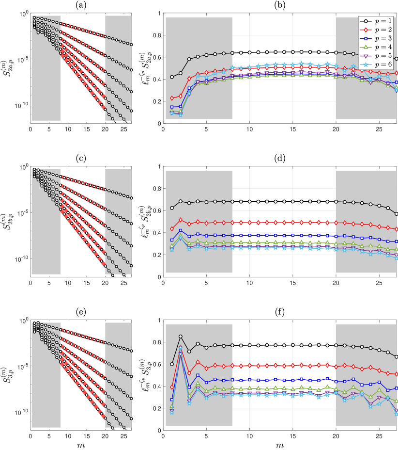
Figure 2: Same plots as in Fig. 1 for the multi-time structure functions: (a,b) $S_{2a,p}^{(m)}$, (c,d) $S_{2b,p}^{(m)}$, (e,f) $S_{3,p}^{(m)}$.

Another example of a time-scale homogeneous observable of degree $p$ is

$$O_{2b}[u(\cdot)]=|u_{0}(\Delta)|^{p/2}|u_{1}(0)|^{p/2}.$$ (45)

The respective family of observables (13) takes the form

$$O_{2b}^{(h,m,t)}[u(\cdot)]=\ell_{m}^{-2h}\,|u_{m}(t)|^{p/2}\big{|}u_{m+1}\big{(}t+\Delta^{(m,t)}\big{)}\big{|}^{p/2}.$$ (46)

The self-similarity relation (38) yields the two-time two-scale correlation function

$$S_{2b,p}^{(m)}=\Big{\langle}|u_{m}(t)|^{p/2}\big{|}u_{m+1}\big{(}t+\Delta^{(m,t)}\big{)}\big{|}^{p/2}\Big{\rangle}_{t}=f_{p}\,C[O_{2b}]\,\ell_{m}^{\zeta_{p}}.$$ (47)

We test this self-similarity relation in Figs. 2(c,d).

In the third example, we consider the three-time observable

$$O_{3}[u(\cdot)]=|u_{0}(0)|^{p/3}|u_{0}(\Delta)|^{p/3}|u_{0}(2\Delta)|^{p/3},$$ (48)

which is time-scale homogeneous of degree $p$. The resulting self-similarity relation reads

$$S_{3,p}^{(m)}=\Big{\langle}|u_{m}(t)|^{p/3}\big{|}u_{m}\big{(}t+\Delta^{(m,t)}\big{)}\big{|}^{p/3}\big{|}u_{m}\big{(}t+2\Delta^{(m,t)}\big{)}\big{|}^{p/3}\Big{\rangle}_{t}=f_{p}\,C[O_{3}]\,\ell_{m}^{\zeta_{p}}.$$ (49)

This self-similarity relation is verified in Figs. 2(e,f).

Other multi-time and multi-scale observables, which have the property of time-scale homogeneity, can be designed in a similar manner by changing the velocity terms and the time delays. For example, one can use $\Delta=1/|u(0)|$, which yields $\Delta^{(m,t)}=\ell_{m}/|u_{m}(t)|$. Another approach is to use observables that are integrated over time rather than dependent on specific time instants. For example, the observable

$$O[u(\cdot)]=\int_{0}^{\Delta}\big{|}u_{0}(0)\big{|}^{p_{1}}\big{|}u_{0}(s)\big{|}^{p_{2}}ds$$ (50)

is time-scale homogeneous of degree $p=p_{1}+p_{2}-1$. Then one derives

$$O^{(h,m,t)}[u(\cdot)]=\ell_{m}^{-1-hp}\int_{0}^{\Delta^{(m,t)}}\big{|}u_{m}(t)\big{|}^{p_{1}}\big{|}u_{m}(t+s)\big{|}^{p_{2}}ds.$$ (51)

The respective self-similarity rule (38) yields

$$\Big{\langle}\int_{0}^{\Delta^{(m,t)}}\big{|}u_{m}(t)\big{|}^{p_{1}}\big{|}u_{m}(t+s)\big{|}^{p_{2}}ds\Big{\rangle}_{t}\propto\ell_{m}^{1+\zeta_{p}}.$$ (52)

The upper limit of the inetegral can also be replaced by any multiple of $\Delta^{(m,t)}$ or, if convergent, by infinity. Power laws of similar kind were derived in several previous works [16, 4, 24, 26, 27] for average decorrelation times of fluctuations. Our self-similarity relation (38) unifies these power laws through their relation to time-scale homogeneous observables.

V.3 Single-time Kolmogorov multipliers

In this subsection we consider the self-similarity relation (39) corresponding to the special case $p=0$. Using this relation we explain a universal self-similar statistics of Kolmogorov multipliers. Such properties of Kolmogorov multipliers were detected and analyzed numerically in several previous works [1, 9, 6, 29], and their connection with hidden symmetry was revealed in [21, 23, 22].

The Kolmogorov multiplier at shell $m$ and time $t$ is defines as

$$w_{m}(t)=\left|\frac{u_{m}(t)}{u_{m-1}(t)}\right|.$$ (53)

Let us define the observables

$$O[u(\cdot)]=f\left(\left|\frac{u_{0}(0)}{u_{-1}(0)}\right|\right)\quad\Rightarrow\quad O^{(0,m,t)}[u(\cdot)]=f\left(\left|\frac{u_{m}(t)}{u_{m-1}(t)}\right|\right)=f\big{(}w_{m}(t)\big{)}.$$ (54)

One can see that $O$ is time-scale homogeneous of degree $0$ for any function $f:\mathbb{R}\mapsto\mathbb{R}$. The cumulative distribution function of the multiplier $F_{m}(x)=\mathrm{P}(w_{m}\leq x)$ is obtained as the average

$$F_{m}(x)=\big{\langle}O^{(0,m,t)}\big{\rangle}_{t},$$ (55)

where the observable is given by Eq. (54) with the indicator function $f=\mathbf{1}_{[0,x]}$. Using the self-similarity relation (39), we conclude that the multipliers have the same probability distribution at all shells of the inertial interval, and this distribution is universal with respect to forcing and viscosity. This conclusion naturally extends to a mutual distributions of several multipliers.

Similar argument applies to the phases multipliers defined as [1, 9]

$$\varphi_{m}(t)=\arg\big{[}u_{m-1}(t)u_{m}(t)u_{m+1}^{*}(t)\big{]}.$$ (56)

In this case we choose the observables

$$O[u(\cdot)]=f\big{(}\arg\left[u_{-1}(0)u_{0}(0)u_{1}^{*}(0)\right]\big{)}\quad\Rightarrow\quad O^{(0,m,t)}[u(\cdot)]=f\big{(}\varphi_{m}(t)\big{)}.$$ (57)

Again, one can see that $O$ is time-scale homogeneous of degree $0$. The cumulative distribution function of the phase multiplier is obtained by the same average (55) applied to the observables (57) with the indicator function $f=\mathbf{1}_{[-\pi,x]}$. The self-similarity rule (39) states that the probability distributions of phase multipliers are scale-independent in the inertial interval.

V.4 Multi-time Kolmogorov multipliers

Let us now extend the results of the previous subsection to multi-time multipliers. Using the turnover times $\Delta$ and $\Delta^{(m,t)}$ from Eqs. (41) and (43), we define

$$O[u(\cdot)]=f\left(\frac{u_{0}(\Delta)}{u_{0}(0)}\right)\quad\Rightarrow\quad O^{(0,m,t)}[u(\cdot)]=f\left(\frac{u_{m}\big{(}t+\Delta^{(m,t)}\big{)}}{u_{m}(t)}\right).$$ (58)

The observable $O^{(0,m,t)}$ corresponds to the two-time complex multiplier

$$\hat{w}_{m}(t)=\frac{u_{m}\big{(}t+\Delta^{(m,t)}\big{)}}{u_{m}(t)},$$ (59)

which measures the relative change of the shell variable $u_{m}(t)$ over one turnover time. The probability distribution of this multiplier can be expressed as

$$\mathrm{P}_{m}(\hat{w}_{m}\in A)=\big{\langle}O^{(0,m,t)}\big{\rangle}_{t},$$ (60)

where $A\subset\mathbb{C}$ is a measurable set and $f=\mathbf{1}_{A}$ is the corresponding indicator function. Then the self-similarity relation (39) states that this probability distributions does not depend on scale in the inertial interval.

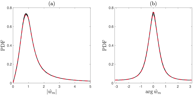
Figure 3: Solid black lines are PDFs for (a) absolute values and (b) phases of two-time complex multipliers $\hat{w}_{m}(t)$. Each panel shows eleven (almost undistinguishable) PDFs for $m=8,\ldots,18$. Dashed red lines show the same PDFs for $m=11$ and different boundary conditions (61).

Using numerical simulations, we plot in Fig. 3 the probability density functions (PDFs) for the absolute values (left panel) and the phases (right panel) of the multiples (59). These graphs confirm that the PDFs indeed collapse for the shells $m=8,\ldots,18$ from the inertial interval.

V.5 Universality with respect to viscosity and forcing

It is generally assumed that the statistically stationary state is independent of the Reynolds number outside the dissipation range, i.e., at scales of the inertial interval and the forcing range. In particular, such independence for the exponents $\zeta_{p}$ and prefactors in anomalous scaling laws (40) was verified numerically in [17]. Analogous study for the rescaled variables $U_{N}^{(m)}(\tau)$ was carried out in [22]. For our self-similarity relation (38), this implies that both prefactors $f_{p}$ and $C[O]$ are universal with respect to dissipation (viscosity). As an example, let us consider the two-time structure function $S_{2b,p}^{(m)}$ from Eq. (47). Figure 4(a) shows the compensated values $\ell_{m}^{-\zeta_{p}}S_{2b,p}^{(m)}$ for $p=5$ evaluated numerically with the increasing Reynolds numbers $\mathrm{Re}=10^{8}$, $10^{10}$ and $10^{12}$. This graphs demonstrate the convergence to the same constant value in the increasing inertial interval.

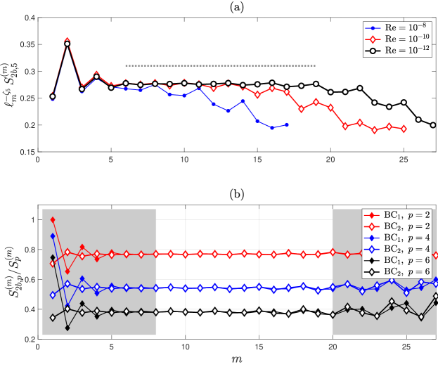
Figure 4: (a) Compensated values $\ell_{m}^{-\zeta_{p}}S_{2b,p}^{(m)}$ of the two-time structure function (47) of order $p=5$. Numerical results with increasing Reynolds numbers demonstrate convergence to the same constant value in an increasing inertial interval. A dotted constant line is shown for visual reference. (b) Ratios $S_{2b,p}^{(m)}/S_{p}^{(m)}$ of the structure functions for two different boundary conditions, $\mathrm{BC}_{1}$ and $\mathrm{BC}_{2}$. Their values converge to the same constant in the inertial interval for every $p=2,4$ and $6$.

Unlike viscosity, the change of forcing (boundary) conditions affects the statistically stationary state globally. Universal properties with respect to forcing for single-time structure functions were studied in [18], and here we extend these results to multi-time statistics. For numerical tests, we use the second boundary condition of the form

$$u_{0}(t)\equiv 1/2,\quad u_{-1}(t)\equiv 1,\quad u_{n}(t)\equiv 0,\quad n<-1.$$ (61)

The only forcing-dependent part of our self-similarity relation (38) is the prefactor $f_{p}$. It depends on the degree of homogeneity $p$, but not on a specific form of the observable. The other coefficient $C[O]$ in Eq. (38) does not depend on the forcing, but depends on the observable. We test these properties by measuring the ratio of expressions (38) for two different observables of the same degree $p$. Then the forcing-dependent factor $f_{p}$ cancels out and hence the ratio becomes independent of the forcing. We confirm this independence numerically in Fig. 4(b) by plotting the ratios

$$\frac{S_{2b,p}^{(m)}}{S_{p}^{(m)}}=\frac{C[O_{2b}]}{C[O]}$$ (62)

of the two- and one-time structure functions from Eqs. (47) and (40). The figure confirms that the ratios (62) coincide asymptotically in the inertial interval for two different boundary conditions: $\mathrm{BC}_{1}$ from Eq. (3) and $\mathrm{BC}_{2}$ from (61).

It is also interesting to see how the prefactor $f_{p}$ changes with the change of forcing (boundary conditions). We denote by $f_{p}^{\mathrm{BC}_{1}}$ and $f_{p}^{\mathrm{BC}_{2}}$ its values for the two boundary conditions under consideration. We find their ratio using the structure functions (40) and (47) as

$$\frac{f_{p}^{\mathrm{BC}_{1}}}{f_{p}^{\mathrm{BC}_{2}}}=\frac{S_{p}^{(m)}\textrm{ for }\mathrm{BC}_{1}}{S_{p}^{(m)}\textrm{ for }\mathrm{BC}_{2}}=\frac{S_{2b,p}^{(m)}\textrm{ for }\mathrm{BC}_{1}}{S_{2b,p}^{(m)}\textrm{ for }\mathrm{BC}_{2}}.$$ (63)

Here we specified that the structure functions in numerators and denominators are computed for $\mathrm{BC}_{1}$ and $\mathrm{BC}_{2}$, respectively. The ratios (63) obtained by numerical simulations for $m=11$ are presented in Fig. 5. They coincide for the one- and two-time structure functions, as predicted by Eq. (63). The inset shows the same plots on a vertical logarithmic scale, from which we conclude that the dependence of the ratios (63) on $p$ is not a power law. In particular, the dependence of $f_{p}$ on forcing cannot be reduced to a power of a single physical quantity (such as the energy flux [18]).

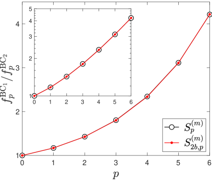
Figure 5: Ratios of forcing-dependent prefactors $f_{p}^{\mathrm{BC}_{1}}/f_{p}^{\mathrm{BC}_{2}}$ for $p=0,\ldots,6$ and fixed shell $m=11$. The inset shows the same plots on a vertical logarithmic scale.

Finally, for $p=0$ the self-similarity rule (39) is universal with respect to the forcing mechanism. According to Sections V.3 and V.4, this implies that the statistics of multipliers does not depend on forcing. For one-time Kolmogorov multiples, this observation goes back to earlier works [1, 9]. Dashed red lines in Fig. 3 verify this universality for the two-time multiplier (59).

VI Derivation of the self-similarity relation

This section presents the derivation of the self-similarity relation (38) and its special case (39) from the hidden scale invariance. For convenience, we divide this derivation into four steps, considered in the following subsections. The first steps relates $\mathcal{P}$ to another projector. The second steps express the observable $O^{(h,m,t)}$ in terms of a proper observable $O_{\star}^{(m,\tau)}$ for rescaled solutions. The third step does the same for their time averages. The derivation is completed in the fourth step, where we use the statistics of multipliers expressed in terms of Perron–Frobenius modes.

Our derivation is based on formal assumptions about the developed turbulent state: existence of the inertial interval, the restored hidden symmetry, ergodicity and Perron–Frobenius asymptotics. Because of these assumptions, our derivation does not reach the level of a rigorous mathematical proof. A possible direction towards a rigorous proof is to use the limit (35), which should be understood in a proper functional setting.

VI.1 Relationship between projectors

Let us introduce the operator

$$\mathcal{R}:{u}(\cdot)\mapsto\hat{u}(\cdot),\quad\hat{u}(r)=\frac{1}{A[{u}(0)]}\,u\left(\frac{r}{A[{u}(0)]}\right).$$ (64)

One can check using Eq. (21) that $A[\hat{u}(0)]=1$ and hence $\mathcal{R}[\hat{u}(\cdot)]=\hat{u}(\cdot)$. This means that $\mathcal{R}$ is a projector. In this subsection we prove that, if $u(t)$ solves the ideal system (5), then the projectors $\mathcal{R}$ and $\mathcal{P}$ are related as

$$\mathcal{R}=\mathcal{Q}\circ\mathcal{P}.$$ (65)

The transition operator $\mathcal{Q}$ acting on $U(\cdot)=\mathcal{P}[u(\cdot)]$ is defined as

$$\mathcal{Q}:U(\cdot)\mapsto\hat{u}(\cdot),\quad\hat{u}(r)=w(\tau)U(\tau),\quad r=\int_{0}^{\tau}\frac{ds}{w(s)},\quad w(\tau)=\exp\bigg{(}\int_{0}^{\tau}R[U(s)]ds\bigg{)},$$ (66)

with the function $R[U]$ from Eq. (30). The operator (66) combines the time-dependent scaling of the state with the transformation of times $\tau\mapsto r$.

Let us proceed with the derivation. Let $U(\cdot)=\mathcal{P}[u(\cdot)]$. First, we derive the useful identify

$$w(\tau)=\frac{A[u(t)]}{A[u(0)]},$$ (67)

where $\tau$ is given by Eq. (20). Expressing $w(\tau)$ from Eq. (66) and $R[U]$ from Eq. (30), we obtain

$$\begin{array}[]{rcl}\displaystyle\frac{d}{d\tau}\log w(\tau)&=&\displaystyle\sum_{j\geq 0}8^{-j}\Re\left(U^{*}_{-j}(\tau)B_{-j}[U(\tau)]\right)=\frac{1}{A^{3}[u(t)]}\sum_{j\geq 0}8^{-j}\Re\left(u^{*}_{-j}(t)B_{-j}[u(t)]\right)\\[17.0pt] &=&\displaystyle\frac{1}{A^{2}[u(t)]}\frac{d}{dt}A[u(t)]=\frac{1}{A[u(t)]}\frac{d}{dt}\log\frac{A[u(t)]}{A[u(0)]}.\end{array}$$ (68)

In this derivation, the second equality used expressions (20) with the quadratic form of the nonlinear term (2), while the third equality follows from the expression (21) and the ideal system (5). Integrating the left-hand side of Eq. (68) with respect to $\tau$ yields $\log w(\tau)$. Expressing $d\tau=A[u(t)]\,dt$ from Eq. (20), the same integration in the right-hand side of Eq. (68) yields $\log\big{(}A[u(t)]/A[u(0)]\big{)}$. This proves the identity (67).

Let us now consider the operator $\mathcal{R}$. Using Eq. (67) with relations (20), we express the function $\hat{u}(r)$ from Eq. (64) for $r=A[u(0)]t$ as

$$\hat{u}(r)=\frac{A[u(t)]}{A[u(0)]}\frac{u(t)}{A[u(t)]}=w(\tau)U(\tau),\quad\tau=\int_{0}^{t}A[u(s)]\,ds=\int_{0}^{r/A[u(0)]}A[u(s)]\,ds.$$ (69)

Differentiating the second relation with the use of $t=r/A[u(0)]$ and Eq. (67) yields

$$\frac{d\tau}{dr}=\frac{A[u(r/A[u(0)])]}{A[u(0)]}=\frac{A[u(t)]}{A[u(0)]}=w(\tau).$$ (70)

This equality is integrated as

$$r=\int_{0}^{\tau}\frac{ds}{w(s)}.$$ (71)

Combining Eqs. (69) and (71) with the definitions (64) and (66), we recover Eq. (65) as

$$\mathcal{R}[u(\cdot)]=\hat{u}(\cdot)=\mathcal{Q}[U(\cdot)]=\mathcal{Q}\circ\mathcal{P}[u(\cdot)].$$ (72)

VI.2 Reduction to a rescaled-velocity observable

Let now $u(t)$ be a solution of the viscous shell model (1), $U(\cdot)=\mathcal{P}[u(\cdot)]$ be the corresponding rescaled solution, and $O$ be a time-scale homogeneous observable of degree $p$. In this subsection we prove the relation

$$A_{m}^{-p}(t)\,O^{(h,m,t)}[u(\cdot)]=\ell_{m}^{(1-h)p}\,O_{\star}^{(m,\tau)}[U(\cdot)]$$ (73)

for any inertial interval observable $O^{(h,m,t)}$. Here $A_{m}(t)$ and $\tau$ are given by Eq. (28) and

$$O_{\star}=O\circ\mathcal{Q}$$ (74)

with the operator $\mathcal{Q}$ defined by Eq. (66).

For the derivation we proceed as follows. Using Eqs. (13) and (10) with property (36) we write

$$O^{(h,m,t)}=O\circ\mathcal{S}_{h}^{m}\circ\Phi^{t}=O\circ\mathcal{T}^{\ell_{m}^{h-1}}\circ\mathcal{S}^{m}\circ\Phi^{t}=\ell_{m}^{(1-h)p}\,O\circ\mathcal{S}^{m}\circ\Phi^{t}.$$ (75)

Since $\mathcal{T}^{\alpha}\circ\mathcal{T}^{1/\alpha}$ is the identity for any $\alpha>0$, we similarly express

$$O=O\circ\mathcal{T}^{\alpha}\circ\mathcal{T}^{1/\alpha}=\alpha^{-p}O\circ\mathcal{T}^{1/\alpha}.$$ (76)

Combining Eqs. (75) and (76) and taking $\alpha=1/A_{m}(t)$, we obtain

$$O^{(h,m,t)}[u(\cdot)]=\ell_{m}^{(1-h)p}A_{m}^{p}(t)\,O\circ\mathcal{T}^{A_{m}(t)}\circ\mathcal{S}^{m}\circ\Phi^{t}[u(\cdot)].$$ (77)

Using Eqs. (7) and (9) we write

$$\tilde{u}(\cdot)=\mathcal{S}^{m}\circ\Phi^{t}[u(\cdot)],\quad\tilde{u}_{n}(s)=\frac{u_{m+n}(s+t)}{\ell_{m}}.$$ (78)

Then, using Eqs. (21) and (28) we express

$$A_{m}(t)=A[\tilde{u}(0)].$$ (79)

This relation combined with the definition (8) yield

$$\mathcal{T}^{A_{m}(t)}[\tilde{u}(\cdot)]=\mathcal{R}[\tilde{u}(\cdot)],$$ (80)

where the operator $\mathcal{R}$ is defined in Eq. (64).

Since our relations refer to inertial interval observables, we can assume the ideal system (5) to be valid in all calculations. Hence, we can use the identity (65). Combining Eqs. (77), (78), (80) with (65), yields

$$\begin{array}[]{rcl}A_{m}^{-p}(t)\,O^{(h,m,t)}[u(\cdot)]&=&\ell_{m}^{(1-h)p}\,O\circ\mathcal{R}[\tilde{u}(\cdot)]=\ell_{m}^{(1-h)p}\,O\circ\mathcal{Q}\circ\mathcal{P}[\tilde{u}(\cdot)]\\[5.0pt] &=&\ell_{m}^{(1-h)p}\,O\circ\mathcal{Q}\circ\mathcal{P}\circ\mathcal{S}^{m}\circ\Phi^{t}[u(\cdot)]=\ell_{m}^{(1-h)p}\,O_{\star}\circ\mathcal{P}\circ\mathcal{S}^{m}\circ\Phi^{t}[u(\cdot)],\end{array}$$ (81)

where we substituted the definition (74) in the last equality. Using the commutation relations (12), (24) and (29), we have

$$\mathcal{P}\circ\mathcal{S}^{m}\circ\Phi^{t}[u(\cdot)]=\mathcal{P}\circ\Phi^{t}\circ\mathcal{S}^{m}[u(\cdot)]=\Phi^{\tau}\circ\mathcal{P}\circ\mathcal{S}^{m}[u(\cdot)]=\Phi^{\tau}\circ\mathcal{H}^{m}\circ\mathcal{P}[u(\cdot)]=\Phi^{\tau}\circ\mathcal{H}^{m}[U(\cdot)].$$ (82)

Substituting this relation into Eq. (81) and recalling the definition (31) yields Eq. (73).

VI.3 Relation between mean values

In this subsection we prove the relation

$$\big{\langle}O^{(h,m,t)}\big{\rangle}_{t}=\frac{\ell_{m}^{-ph}}{c_{m}}\Big{\langle}\Big{(}\prod_{N=-m+1}^{0}X_{N\star}^{(m,\tau)}\Big{)}^{p-1}O_{\star}^{(m,\tau)}\Big{\rangle}_{\tau},\quad c_{m}=\Big{\langle}\Big{(}\prod_{N=-m+1}^{0}X_{N\star}^{(m,\tau)}\Big{)}^{-1}\Big{\rangle}_{\tau},$$ (83)

where the observables $X_{N\star}:U(\cdot)\mapsto\mathbb{R}$ are defined as

$$X_{N\star}[U(\cdot)]=\sqrt{8^{-1}+\frac{8^{-1}|U_{N}[0]|^{2}}{\sum_{j\geq 1}8^{-j}|U_{N-j}(0)|^{2}}}.$$ (84)

For the derivation, let us first show that

$$\frac{A_{m+N}(t)}{A_{m+N-1}(t)}=2X_{N\star}^{(m,\tau)}[U(\cdot)],\quad\tau=\int_{0}^{t}A_{m}(s)ds.$$ (85)

These expressions describe a specific type of multipliers defined as ratios of the amplitudes $A_{m}(t)$ [20]. By definition (31), we have $X_{N\star}^{(m,\tau)}=X_{N\star}\circ\Phi^{\tau}\circ\mathcal{H}^{m}$. Using Eqs. (32), (84) and (28), elementary maniplations yield Eq. (85) as

$$\begin{array}[]{rcl}X_{N\star}^{(m,\tau)}[U(\cdot)]&=&\displaystyle\sqrt{8^{-1}+\frac{8^{-1}|U_{N}^{(m)}[\tau]|^{2}}{\sum_{j\geq 1}8^{-j}|U_{N-j}^{(m)}(\tau)|^{2}}}=\sqrt{\frac{8^{-1}\sum_{j\geq 0}8^{-j}|U_{N-j}^{(m)}(\tau)|^{2}}{\sum_{j\geq 1}8^{-j}|U_{N-j}^{(m)}(\tau)|^{2}}}\\[20.0pt] &=&\displaystyle\sqrt{\frac{\sum_{j\geq 0}8^{-j}|U_{N-j}^{(m)}(\tau)|^{2}}{\sum_{j\geq 0}8^{-j}|U_{N-1-j}^{(m)}(\tau)|^{2}}}=\sqrt{\frac{\sum_{j\geq 0}8^{-j}|u_{m+N-j}(t)|^{2}}{\sum_{j\geq 0}8^{-j}|u_{m+N-1-j}(t)|^{2}}}\\[20.0pt] &=&\displaystyle\frac{\ell_{m+N}A_{m+N}(t)}{\ell_{m+N-1}A_{m+N-1}(t)}=\frac{A_{m+N}(t)}{2A_{m+N-1}(t)}.\end{array}$$ (86)

Recall that $A_{0}(t)\equiv 1$ for the boundary conditions (3). Hence, using Eq. (85) we factorize

$$A_{m}(t)=\prod_{N=-m+1}^{0}\frac{A_{m+N}(t)}{A_{m+N-1}(t)}=\frac{1}{\ell_{m}}\prod_{N=-m+1}^{0}X_{N\star}^{(m,\tau)}[U(\cdot)].$$ (87)

Using Eq. (87) we express the observable $O^{(h,m,t)}$ from Eq. (73) as

$$O^{(h,m,t)}[u(\cdot)]=\ell_{m}^{-ph}\,\bigg{(}\prod_{N=-m+1}^{0}X_{N\star}^{(m,\tau)}[U(\cdot)]\bigg{)}^{p}O_{\star}^{(m,\tau)}[U(\cdot)].$$ (88)

Similarly, we write the relation between the times, $d\tau=A_{m}(t)dt$ from Eq. (28), as

$$dt=\ell_{m}\bigg{(}\prod_{N=-m+1}^{0}X_{N\star}^{(m,\tau)}[U(\cdot)]\bigg{)}^{-1}d\tau.$$ (89)

Using Eqs. (88) and (89), we express the average of $O^{(h,m,t)}$ in the form

$$\begin{array}[]{rcl}\big{\langle}O^{(h,m,t)}\big{\rangle}_{t}&=&\displaystyle\lim_{T\to\infty}\frac{\int_{0}^{T}O^{(h,m,t)}[u(\cdot)]dt}{\int_{0}^{T}dt}\\[20.0pt] &=&\displaystyle\ell_{m}^{-ph}\lim_{\tilde{T}\to\infty}\frac{\int_{0}^{\tilde{T}}\bigg{(}\prod_{N=-m+1}^{0}X_{N\star}^{(m,\tau)}[U(\cdot)]\bigg{)}^{p-1}O_{\star}^{(m,\tau)}[U(\cdot)]\,d\tau}{\int_{0}^{\tilde{T}}\bigg{(}\prod_{N=-m+1}^{0}X_{N\star}^{(m,\tau)}[U(\cdot)]\bigg{)}^{-1}d\tau},\end{array}$$ (90)

where the second equality is obtained by changing the integration time, $dt\mapsto d\tau$, with the corresponding integration limit $\tilde{T}=\int_{0}^{T}A_{m}(s)ds\to\infty$ as $T\to\infty$. Dividing the numerator and denominator by $\tilde{T}$ and taking a separate limit $\tilde{T}\to\infty$ above and below, one obtains relation (83).

VI.4 Integration using Perron–Frobenius modes

Let $x_{N}^{(m)}$ be a random variable whose distribution is determined by the stationary statistics of the observable $X_{N\star}^{(m,\tau)}[U(\cdot)]$. These observables are well-defined for $N\geq-m+1$. Without loss of generality we can set $x_{N}^{(m)}\equiv 1$ for $N\leq-m$. We denote a joint probability measure for these variables as $d\mu^{(m)}(x_{\ominus})$, where $x_{\ominus}=\big{(}x_{0},x_{-1},x_{-2},\ldots\big{)}$. Note that we have omitted the superscript $(m)$ for the arguments since it is present in the measure notation. Next, we introduce the measures

$$d\mu_{p}^{(m)}(x_{\ominus})=\frac{1}{c_{m}}\bigg{(}\prod_{N=-m+1}^{0}x_{N}\bigg{)}^{p-1}d\mu^{(m)}(x_{\ominus}),\quad c_{m}=\int\bigg{(}\prod_{N=-m+1}^{0}x_{N}\bigg{)}^{-1}d\mu^{(m)}(x_{\ominus}).$$ (91)

Using these measures, we write Eq. (83) as the integral

$$\big{\langle}O^{(h,m,t)}\big{\rangle}_{t}=\ell_{m}^{-ph}\int\big{\langle}O_{\star}^{(m,\tau)}\big{|}x_{\ominus}\big{\rangle}_{\tau}d\mu_{p}^{(m)}(x_{\ominus}),$$ (92)

where $\big{\langle}O_{\star}^{(m,\tau)}\big{|}x_{\ominus}\big{\rangle}_{\tau}$ denotes the conditional average of the observable $O_{\star}^{(m,\tau)}$.

According to Eq. (86), the observable $X_{N\star}^{(m,\tau)}$ is determined by the rescaled velocity $U_{N}^{(m)}(\tau)$ and its close neighbors. Whenever $O_{\star}^{(m,\tau)}$ is the inertial interval observable, its conditional average $\big{\langle}O_{\star}^{(m,\tau)}\big{|}x_{\ominus}\big{\rangle}_{\tau}$ depends only on the components of $x_{\ominus}$ from the inertial interval. In this case the hidden symmetry assumption (34) extends to the conditional averages, i.e., $\big{\langle}O_{\star}^{(m,\tau)}\big{|}x_{\ominus}\big{\rangle}_{\tau}$ does not depend on $m$. Additionally, the universality of the hidden-symmetric state implies the universality of $\big{\langle}O_{\star}^{(m,\tau)}\big{|}x_{\ominus}\big{\rangle}_{\tau}$ with respect to forcing and dissipation. Our derivation using Eq. (92) now relies on computing the measure $d\mu_{p}^{(m)}\big{(}x_{\ominus}\big{)}$ restricted to the inertial interval. This measure describes the amplitude multipliers and therefore does not depend on the observable, except for its dependence on the degree of homogeneity $p$.

In earlier works [20, 21, 22] we used the hidden symmetry hypothesis and derived the asymptotic form of the measure (91) in the inertial interval as

$$d\mu_{p}^{(m)}(x_{\ominus})\approx f_{p}\,\lambda_{p}^{m}\,d\nu_{p}(x_{\ominus}).$$ (93)

Here the quantity $\lambda_{p}>0$ is the Perron–Frobenius eigenvalue and $d\nu_{p}(x_{\ominus})$ is the corresponding eigenvector (probability measure), which are defined for specific positive operators in the framework of the statistically restored hidden symmetry. Both $\lambda_{p}$ and $d\nu_{p}(x_{\ominus})$ are universal together with the hidden-symmetric state. The coefficient $f_{p}$ is not universal and depends on the forcing and degree of homogeneity $p$. In the case $p=0$, Eq. (91) defines $d\mu_{p}^{(m)}(x_{\ominus})$ as a probability measure. Then, Eq. (93) determines

$$f_{0}=\lambda_{0}=1.$$ (94)

We do not repeat these derivations here and refer the reader to [22, Sec. III D] for details.

Substituting the asymptotic form (93) into Eq. (92) yields the self-similarity relation (38) with

$$\zeta_{p}=-\log_{2}\lambda_{p},\quad C[O]=\int\big{\langle}O_{\star}^{(m,\tau)}\big{|}x_{\ominus}\big{\rangle}_{\tau}d\nu_{p}(x_{\ominus}).$$ (95)

The quantity $C[O]$ does not depend on $m$ and is universal due to the identical properties of both $\big{\langle}O_{\star}^{(m,\tau)}\big{|}x_{\ominus}\big{\rangle}_{\tau}$ and $d\nu_{p}(x_{\ominus})$. Then the relation (39) for $p=0$ follows from Eq. (94).

VII Conclusion

Equations of the ideal (inviscid) Sabra shell model can be transformed by rescaling all variables and time with respect to the instantaneous turnover time at a given scale. The resulting system acquires a hidden symmetry that results from the fusion of the original space-time scaling symmetries. It was conjectured and confirmed numerically that the hidden symmetry is restored in the statistical sense within the inertial interval of the developed turbulence [19]. As a consequence, the anomalous scaling exponents of structure functions were obtained as the Perron–Frobenius eigenvalues of some positive operators based on hidden-symmetric statistics [21, 22]. These results were extended to the Navier–Stokes turbulence in [20, 23].

In this paper we derived a consequence of the restored hidden symmetry for the general (multi-time and multi-scale) statistics of the original variables and time. It is formulated in terms of observables that are homogeneous with respect to time scaling. Any such observable is shown to be self-similar in the inertial interval with the Hölder exponent $h=\zeta_{p}/p$, where $p$ is the degree of homogeneity and $\zeta_{p}$ is the usual anomalous exponent. In the derivation, we develop and use an operator formalism for symmetries, in which the rescaling procedure is represented as a projection.

As applications, we derive scaling rules for multi-time structure functions and explain universality properties of multi-time Kolmogorov multipliers. Here the condition of time-scale homogeneity requires that time differences in multi-time self-similar observables are measured in terms of instantaneous (time-dependent) turnover times. We construct examples of such observables and confirm their self-similarity by accurate numerical simulations.

Acknowledgments. This work was supported by CNPq grant 308721/2021-7, FAPERJ grant E-26/201.054/2022 and CAPES MATH-AmSud project CHA2MAN.

References

- [1] R. Benzi, L. Biferale, and G. Parisi. On intermittency in a cascade model for turbulence. Physica D, 65(1-2):163–171, 1993.
- [2] R. Benzi, L. Biferale, and M. Sbragaglia. A Gibbs-like measure for single-time, multi-scale energy transfer in stochastic signals and Shell Model of turbulence. Journal of Statistical Physics, 114:137–154, 2004.
- [3] L. Biferale. Shell models of energy cascade in turbulence. Annual Review of Fluid Mechanics, 35:441–468, 2003.
- [4] L. Biferale, G. Boffetta, A. Celani, and F. Toschi. Multi-time, multi-scale correlation functions in turbulence and in turbulent models. Physica D, 127(3-4):187–197, 1999.
- [5] L. Biferale, E. Calzavarini, and F. Toschi. Multi-time multi-scale correlation functions in hydrodynamic turbulence. Physics of Fluids, 23(8), 2011.
- [6] L. Biferale, A. A. Mailybaev, and G. Parisi. Optimal subgrid scheme for shell models of turbulence. Physical Review E, 95(4):043108, 2017.
- [7] X. M. de Wit, G. Ortali, A. Corbetta, A. A. Mailybaev, L. Biferale, and F. Toschi. Extreme statistics and extreme events in dynamical models of turbulence. Physical Review E, 109(5):055106, 2024.
- [8] J. Domingues Lemos and A. A. Mailybaev. Data-based approach for time-correlated closures of turbulence models. Physical Review E, 109(2):025101, 2024.
- [9] G. L. Eyink, S. Chen, and Q. Chen. Gibbsian hypothesis in turbulence. Journal of Statistical Physics, 113(5-6):719–740, 2003.
- [10] U. Frisch. Turbulence: the Legacy of A.N. Kolmogorov. Cambridge University Press, 1995.
- [11] U. Frisch and M. Vergassola. A prediction of the multifractal model: the intermediate dissipation range. Europhysics Letters, 14:439–444, 1991.
- [12] E. B. Gledzer. System of hydrodynamic type admitting two quadratic integrals of motion. Sov. Phys. Doklady, 18:216, 1973.
- [13] A. N. Kolmogorov. The local structure of turbulence in incompressible viscous fluid for very large Reynolds numbers. Dokl. Akad. Nauk SSSR, 30(4):299–303, 1941.
- [14] V. L’vov and I. Procaccia. Towards a nonperturbative theory of hydrodynamic turbulence: Fusion rules, exact bridge relations, and anomalous viscous scaling functions. Physical Review E, 54(6):6268, 1996.
- [15] V. S. L’vov, E. Podivilov, A. Pomyalov, I. Procaccia, and D. Vandembroucq. Improved shell model of turbulence. Phys. Rev. E, 58(2):1811, 1998.
- [16] V. S. L’vov, E. Podivilov, and I. Procaccia. Temporal multiscaling in hydrodynamic turbulence. Physical Review E, 55(6):7030, 1997.
- [17] V. S. L’vov, I. Procaccia, and D. Vandembroucq. Universal scaling exponents in shell models of turbulence: viscous effects are finite-sized corrections to scaling. Physical Review Letters, 81(4):802, 1998.
- [18] V. S. L’vov, R. A. Pasmanter, A. Pomyalov, and I. Procaccia. Strong universality in forced and decaying turbulence in a shell model. Physical Review E, 67(6):066310, 2003.
- [19] A. A. Mailybaev. Hidden scale invariance of intermittent turbulence in a shell model. Physical Review Fluids, 6(1):L012601, 2021.
- [20] A. A. Mailybaev. Hidden spatiotemporal symmetries and intermittency in turbulence. Nonlinearity, 35:3630–3679, 2022.
- [21] A. A. Mailybaev. Shell model intermittency is the hidden self-similarity. Physical Review Fluids, 7(3):034604, 2022.
- [22] A. A. Mailybaev. Hidden scale invariance of turbulence in a shell model: from forcing to dissipation scales. Physical Review Fluids, 8(5):054605, 2023.
- [23] A. A. Mailybaev and S. Thalabard. Hidden scale invariance in Navier–Stokes intermittency. Philosophical Transactions of the Royal Society A, 380:20210098, 2022.
- [24] D. Mitra and R. Pandit. Varieties of dynamic multiscaling in fluid turbulence. Physical Review Letters, 93(2):024501, 2004.
- [25] K. Ohkitani and M. Yamada. Temporal intermittency in the energy cascade process and local Lyapunov analysis in fully developed model of turbulence. Prog. Theor. Phys., 81(2):329–341, 1989.
- [26] R. Pandit, S. S. Ray, and D. Mitra. Dynamic multiscaling in turbulence. The European Physical Journal B, 64:463–469, 2008.
- [27] S. S. Ray, D. Mitra, and R. Pandit. The universality of dynamic multiscaling in homogeneous, isotropic Navier–Stokes and passive-scalar turbulence. New Journal of Physics, 10(3):033003, 2008.
- [28] T. Rithwik and S. R. Samriddhi. Revisiting the SABRA model: Statics and dynamics. EPL (Europhysics Letters), 120(3), 2017.
- [29] N. Vladimirova, M. Shavit, and G. Falkovich. Fibonacci turbulence. Physical Review X, 11:021063, 2021.