Quantum Down Sampling Filter for Variational Auto-encoder

Abstract

Variational Auto-encoders (VAEs) are crucial for generative modeling and image reconstruction, but their performance often degrades with low-resolution input (16x16 pixels), leading to blurred or inaccurate results. This study proposes a hybrid model that combines quantum computing in the VAE encoder (Q-VAE) and convolutional neural networks (CNNs) in the decoder. By upscaling the resolution from 16x16 to 32x32 during encoding, we assess the model’s ability to preserve key features while improving image resolution. We tested the model on the MNIST and USPS datasets, comparing it to VAE refered as classical VAE (C-VAE) and the classical direct-passing VAE (CDP-VAE), which uses windowing pooling filters. Evaluation using Fréchet Inception Distance (FID) and Mean Squared Error (MSE) shows that the Q-VAE outperforms both, suggesting its potential for image resolution enhancement and synthetic data generation.

1 Introduction

Variational Autoencoders (VAEs) have become foundational tools in generative modeling and image reconstruction, especially in tasks that require efficient and precise feature extraction from high-resolution data [1]. VAEs are part of the broader family of latent-variable models [2], wherein an encoder maps input data to a structured latent space, and a decoder reconstructs the data from this representation. Despite their success in a wide range of applications, VAEs often face challenges as latent space is often not expressive enough to model intricate relationships, often leading to blurry or low-quality output [3]. These limitations arise primarily from the difficulty of capturing complex high-resolution dependencies, which become especially apparent when dealing with large data sets (which consists of millions of images) or complex structures [5].

Recent advancements in quantum computing offer promising avenues for overcoming these challenges by exploiting quantum phenomena such as superposition and entanglement. These properties allow for more efficient data representation and processing, potentially overcoming some of the bottlenecks inherent in classical methods for generative modeling [6]. The integration of quantum circuits into neural networks, particularly within the VAE encoder, has shown potential to improve latent space representations, leading to enhanced feature extraction and more accurate reconstructions [7]. Quantum in VAE represents an example of such hybrid models, which leverage quantum operations to better capture the underlying data structure, making them especially well suited for high-resolution image tasks [6].

Recent advances in generative models have led to the increased use of low-resolution images, such as 8x8 or 16x16 pixels, as starting points for training medium-quality output [8]. This approach might seem counterintuitive because of the small size of these images, but it has proven effective for several reasons. Training generative models on low-resolution images allows for faster training times, as smaller images require less computational power and processing, enabling faster iterations and fine-tuning. In addition, low-resolution images force the model to focus on learning high-level patterns and structures rather than fine-grained details. This simplification helps the model build a strong foundation for understanding the essential features of the data. Once the model has learned to generate meaningful, broad structures at low resolution, it can then be used to upscale or refine the output to a medium resolution, such as 32x32, using techniques like super-resolution or progressive refinement. This method allows the model to generate more detailed and sharper images, while avoiding the computational difficulties that come with directly training on medium resolutions like 32x32.

Although 32x32-pixel images are commonly used in many applications, including image classification and generative modeling, classical models like VAEs struggle with these resolutions due to limitations in their architecture [9]. VAEs operate by encoding input data into a compressed probabilistic latent space that is then used to reconstruct the input image. However, with 32x32 images, the encoder has to condense a large amount of pixel information into a smaller latent space, often losing fine details in the process. This leads to blurred or artifact-filled reconstructions, as the latent space might not capture the complexity of the image at this resolution. The encoder’s limited capacity to represent detailed features in the latent space becomes particularly problematic for 32x32 images, which are still complex enough to contain important texture, color variation, and structural information. As a result, VAEs can struggle to generate high-quality images from these lower-resolution inputs [10]. The use of 32x32 resolution is prevalent in many machine learning applications, particularly in image classification tasks and generative modeling, as it strikes a balance between computational efficiency and sufficient detail. Datasets like CIFAR-10 and CIFAR-100, which consist of 32x32 pixel images, are standard benchmarks for evaluating generative models and classifiers [11]. Additionally, modern generative models often employ techniques like progressive training, where low-resolution images (8x8 or 16x16) are initially learned and then progressively refined to medium resolutions, such as 32x32 or beyond. This process stabilizes training and reduces the complexity associated with generating high-resolution outputs [12]. In practice, combining low-resolution training (e.g., 8x8 or 16x16) with upscaling techniques allows generative models to learn more efficiently and handle the complexities of higher-resolution images. By training on smaller images first, the models can focus on understanding the broader patterns in the data, then gradually increase the resolution to produce more detailed output. This method has potential to be useful for reducing computational load and improving the quality of the final images generated.

In this work, we introduce a novel Q-VAE that integrates quantum encoding techniques in the encoder while using Convolutional Neural Networks (CNNs) in the decoder. This hybrid architecture leverages the high expressiveness of quantum states to improve feature extraction and mitigate the blurriness often associated with classical VAEs. Unlike traditional quantum generative models, which typically operate on lower-resolution datasets (e.g. 8x8 or 16x16 pixels) [12], our approach is designed to handle medium-resolution inputs, such as 32x32 pixels, allowing the model to produce better-quality image reconstructions for more complex datasets. In the context of Q-VAE, we use MNIST and USPS datasets primarily due to their simplicity and relevance to early-stage exploration of quantum models in image generation. Both are grayscale datasets, which are less complex than color images, making them ideal for testing new techniques, particularly when working with emerging technologies like quantum computing in machine learning.

Since quantum computing, especially its integration into deep learning models, is still in the early stages, focusing on simpler datasets allows for a more controlled environment where we can better understand the impact of quantum techniques on model performance. Furthermore, the datasets used in this study, such as MNIST and USPS (with image resolutions of 28x28 and 16x16 pixels, respectively), are relatively small in size, which is advantageous when exploring the potential of quantum circuits for feature extraction and latent space representation. Their reduced resolution helps reduce the computational burden compared to higher-resolution images. To ensure a fair evaluation, the MNIST dataset is first down-sampled from 28x28 to 16x16 pixels, and then, like the USPS dataset, it is up-sampled to 32x32 pixels before being used as input to assess our model’s performance.

By focusing on grayscale images, we reduce the complexity of the problem, allowing for clearer insights into how quantum techniques can improve feature extraction and image reconstruction, particularly for simpler tasks like recognizing digits. Once the approach is successfully validated on these datasets, the methods can be extended to more complex and higher-resolution data, such as color images or higher resolutions.

Quantitative analysis has been performed to compare the effectiveness of the model using common performance metrics, such as the Fréchet Inception Distance (FID) and the Mean Squared Error (MSE), which are essential to assess the quality of generated images and the representation of the latent space [18, 19]. Thus, by leveraging these datasets, we can benchmark the Q-VAE against traditional models,to explore that if quantum component brings measurable improvements to the generative process. In summary the following contributions have been made in this paper:

• Introduces a new model quantum VAE (Q-VAE), where quantum encoding is applied only in the encoder, simplifying the model and improving the feature extraction capabilities.

• Compares Q-VAE with the classical Direct Passing CDP-VAE, highlighting performance differences due to the inclusion of quantum encoding in the encoder.

• Avoids quantum entanglements or layers in the encoder, focusing solely on an efficient quantum encoding circuit for latent space encoding.

• Minimizes quantum-trainable parameters, leading to more efficient model training and better utilization of quantum resources.

• Evaluate whether quantum encoding improves the generative quality and the latent space representation compared to classical methods.

• Investigates whether converting images from low resolution (16x16) to medium resolution (32x32) improves model performance.

The structure of this paper is as follows. Section 2 provides a review of related work on classical VAEs and their integration with quantum computing. Section 3 presents the background on Variational Autoencoders (VAEs). In Section 4, the methodology for the proposed quantum-enhanced VAE model is introduced. Section 5 outlines the numerical simulations conducted, while Section 6 discusses the performance analysis. Finally, Section 7 concludes the paper, summarizing the key findings and suggesting potential avenues for future research.

2 Related Research

In recent years, variational auto-encoders (VAEs) have garnered significant attention in generative modeling, especially for image reconstruction tasks [21]. Traditional VAEs are praised for their ability to encode data into a structured latent space and regenerate approximations of the input. However, classical VAEs often suffer from blurred reconstructions, [3], prompting research to improve VAE architectures for better image quality and feature extraction [25, 26, 27]. Several studies have focused on enhancing VAE performance using convolutional architectures [43, 30, 31, 32]. Gatopoulos et al. introduced convolutional VAEs to better capture image features, surpassing the performance of fully connected architectures in medium-resolution data sets such as CIFAR-10 and ImageNet32 [28]. Furthermore, combining VAE with adversarial training, such as in Adversarial Autoencoders (AAE) [33], incorporates discriminator networks to enhance the visual quality of generated images, address the blurriness issues inherent in classical VAEs, and improve machine learning applications. In addition, anti-adversarial VAEs [34, 35] and VAE-GAN hybrids [36] enhance image generation by incorporating adversarial training, leading to sharper images by reducing blurriness [37].

Quantum Machine Learning (QML) has emerged as a promising field, with studies exploring the integration of quantum circuits into generative models. Quantum GANs (QGANs) leverage quantum computing to enhance the data representation and image generation capabilities of GANs. Although QGANs are not directly related to VAEs, they represent a quantum-based generative approach that improves data diversity and generation quality [39]. Quantum Variational Autoencoders [40, 41, 42, 43, 44, 45] build on the foundational work by Khoshaman et al., who proposed a quantum VAE where the latent generative process is modeled as a quantum Boltzmann machine (QBM). Their approach demonstrates that quantum VAE can be trained end-to-end using a quantum lower bound to the variational log-likelihood, achieving state-of-the-art performance on the MNIST dataset [38]. They have used Log-Likelihood (LL) and Evidence Lower Bound (ELBO) as the measurement and have shown quantum VAE confidence level for the numerical results is smaller than ±0.2 in all cases. Gircha et al. further advanced the quantum VAE architecture by incorporating quantum circuits in both the encoder, which utilizes multiple rotations, and the decoder [42]. These quantum VAE models primarily focus on leveraging quantum methods in the latent space representation, enhancing the generative capabilities of VAEs.

This paper addresses a gap in the literature where quantum techniques are primarily used in hybrid models for the encoder, while the decoder remains classical. Our proposed model is unique in that it leverages quantum encoding with a single rotation gate and measurement solely in the encoder, distinguishing it from other approaches.

3 Background

Variational Auto-encoders (VAEs) are widely recognized as powerful generative models in machine learning. They are based on a probabilistic framework where an encoder network maps input data $\mathbf{x}$ to a latent distribution $q(\mathbf{z}|\mathbf{x})$, and a decoder network reconstructs the data from the latent variables $\mathbf{z}$ as shown in equation 1 [4].

$$L_{\theta,\phi}(x)=\mathbb{E}_{q_{\phi}(z|x)}\left[\log p_{\theta}(x,z)-\log q_{\phi}(z|x)\right]$$ (1)

where $\mathbb{E}_{q(\mathbf{z}|\mathbf{x})}$ represents the expectation with respect to the approximate posterior $q(\mathbf{z}|\mathbf{x})$. The reconstruction term encourages the model to generate data points that are similar to the observed data, while the KL divergence regularizes the learned latent variables by pushing the approximate posterior towards the prior distribution. Although VAEs have been successful in many domains, including image generation and anomaly detection, they often face significant challenges when applied to high-resolution data. This issue can arise because the latent space is often not expressive enough to model the intricate relationships. [14].

3.1 Encoder

A classical VAE encoder is typically implemented as a fully connected network or a Convolutional Neural Network (CNN), with the aim of mapping the input data to a lower-resolution latent space. The primary objective of the encoder is to process the input data $x$, transform it through a series of hidden layers, and output two parameters: the mean $\mu$ and the log variance $\log(\sigma^{2})$, which are used for variational inference [1]. In the case of image data, the input image is first reshaped into a vector and passed through multiple fully connected layers. The transformations performed by these layers help extract important features from the input. For example, given an input image of dimension 1024 (flattened from a $32\times 32$ image), the encoder progressively reduces the resolution’s, often mapping the input image $x_{0}$ into a lower-resolution space $x_{1}$.

3.1.1 CNN or Fully Connected Layers in Encoders

CNNs are particularly useful for image-based data because they can capture local spatial patterns (e.g., edges, textures) by using convolution layers. These convolution layers progressively down-sample the input image and extract high-level features, while the fully connected layers act to compress these features into a more compact latent representation. In CNN-based encoders, after the convolution layers extract relevant patterns, fully connected layers are used to map the high-resolution feature maps into the latent space. This approach allows the model to better capture spatial dependencies while still benefiting from the representational power of fully connected layers.

3.1.2 Windowing and Pooling for Resolution Reduction

Pooling techniques such as max pooling or average pooling play a critical role in reducing the spatial resolution of the input data while retaining important features. In max pooling, for example, the maximum value in a small region (or window) of the input image is selected, effectively reducing the image’s resolution while retaining the most significant features within each region. Average pooling operates similarly, but instead computes the average value of each window. These pooling operations are vital for reducing computational complexity while preserving essential information for later stages of the model. Adaptive pooling is another technique often used in encoders to ensure that feature maps have consistent sizes, regardless of the input size. Adaptive pooling adjusts the pooling operation to produce fixed-sized output maps, which is particularly useful when working with images of varying resolutions. This resolution reduction helps the model focus on more abstract features without losing key information, enabling more efficient learning in the latent space.

3.2 Latent Space Encoding

Finally, the encoder outputs the mean $\mu$ and the log variance $\log(\sigma^{2})$, which parameterize the variational distribution. These are computed as follows:

$$\mu=\text{fc}_{\mu}(h_{2}),$$ (2)

$$\log(\sigma^{2})=\text{fc}_{\log\_var}(h_{2}),$$ (3)

where $\mu$ and $\log(\sigma^{2})$ are vectors of dimension latent_dim, which is 16 in our case.

The proposed architecture effectively combines quantum and classical components, leveraging quantum-enhanced feature extraction for downstream Neural Network processing.

3.3 Decoder

The decoder in a Variational Auto-encoder (VAE) is designed to transform the lower-resolution latent variable $z$, produced by the encoder, back into a high-resolution data space, reconstructing the input data. The decoder typically consists of multiple layers, including fully connected and transposed convolution layers, which progressively reconstruct the input data’s spatial and feature dimensions. The core function of the decoder is to ensure that the reconstructed data match closely the original input, enabling the model to learn both the global structure and the local details of the data. As with the encoder, the decoder is trained to minimize the reconstruction error, often using a loss function that combines both the likelihood of the data given the latent variables and a regularization term that encourages smoothness in the latent-space representation.

3.3.1 Latent Variable Transformation

The decoding process begins by passing the latent variable $z$ through a fully connected layer to map it to a higher resolution feature space. This transformation creates a tensor that matches the expected dimensions for the next layers in the decoder, such as the transposed convolution layers. The fully connected layer enables the decoder to effectively learn a mapping from the compact latent space back to the data space, ensuring that relevant information is maintained during this transformation.

3.3.2 Transposed Convolutions

Once the latent variable is transformed into the higher-resolution space, it is passed through a series of transposed convolution (also known as de-convolution) layers.These layers up-sample the tensor, progressively restoring the original spatial dimensions of the input data. Each transposed convolution layer learns to refine the spatial resolution of the image while preserving important features. Transposed convolution layers have been shown to be highly effective in generating high-resolution outputs from low-resolution latent representations. They are capable of learning hierarchical features of the data, capturing both local details and global structure during the reconstruction process. By applying non-linear activation functions, such as ReLU, between the transposed convolution layers, the model introduces the necessary complexity to capture intricate patterns in the data.

3.3.3 Reconstruction

The final stage of the decoding process involves producing the reconstructed image. This is typically done by passing the output of the last transposed convolution layer through a sigmoid activation function to ensure that the pixel values lie within the valid range (e.g., between 0 and 1 for normalized image data). The output of this step is the reconstructed image, which should ideally match the original input data.

3.4 Quantum Computing in Variational Auto-encoder

Quantum computing has shown promise in enhancing generative models due to its ability to represent information in quantum states. Unlike classical models, which rely on deterministic mappings, quantum encoders can utilize superposition and entanglement to encode data into a potentially much larger computational space, enabling the model to learn richer and more compact latent representations [20]. Quantum circuits can efficiently explore large state spaces, leveraging the Hilbert space to represent data points in ways that are not possible with classical methods [15]. Mathematically, quantum encoders can represent the latent variables $\mathbf{z}$ as quantum states $|\psi\rangle\in\mathcal{H}$, where $\mathcal{H}$ is the Hilbert space. A quantum encoder might take the form of a unitary operator $U_{\theta}$ applied to an initial quantum state $|\mathbf{x}\rangle$, mapping the input data $\mathbf{x}$ to a quantum state that encodes the latent representation that map the medium-dimensional data into a more compact, or lower-dimensional space.

$$|\psi\rangle=U_{\theta}|\mathbf{x}\rangle,$$ (4)

where $U_{\theta}$ is a quantum operation that performs the encoding. This encoding could be leveraged to provide a quantum-enhanced latent space that could more efficiently represent complex structures within the data. Quantum states encoded in this way can capture correlations in data that are hard to model classically, such as in the case of medium-resolution images.

The advantage of quantum properties has potential to improve tasks like image reconstruction and anomaly detection, overcoming challenges like blurred images often encountered with classical VAEs.

4 Proposed Methodology

In this work, we introduce a novel down-sampling filter for quantum variational auto-encoders (Q-VAE) that relies exclusively on quantum encoding for feature extraction. The paper investigates three distinct architectures for Variational Auto-encoders (VAEs), each employing different encoding mechanisms to evaluate their feature extraction capabilities: Quantum VAE (Q-VAE), Classical VAE (C-VAE), and Direct Passing VAE (CDP-VAE). The framework of these models has been presented in Figure 1. The goal of this comparison is to assess the effectiveness of quantum computing, classical neural networks, and simplified encoding strategies in capturing and processing data for subsequent reconstruction. While each model shares a common decoder architecture, the encoders differ in their approach, enabling the study of how each influences the encoding process and the quality of the reconstructed output.

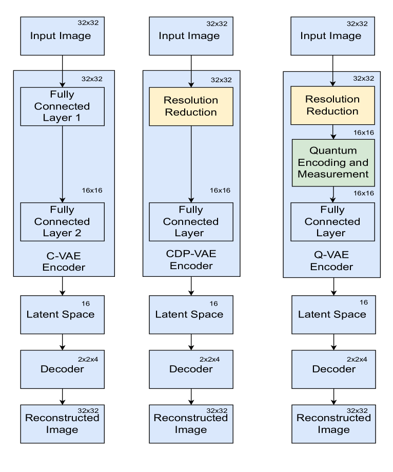
Figure 1: Flowchart for (a) C-VAE, (b) CDP-VAE and (c) Q-VAE.

4.1 Classical VAE (C-VAE) Encoder

The Classical VAE (C-VAE) uses a traditional fully connected neural network as the encoder, which processes the input data through a series of hidden layers to output the mean ($\mu$) and log variance ($\log(\sigma^{2})$) of the latent space distribution. This distribution is then sampled to obtain the latent variable $z$, which represents the encoded data in a lower-resolution space. While the C-VAE relies entirely on classical neural networks for encoding, it remains highly effective in modeling data distributions and is widely used in practical applications. The decoder, typically a CNN, reconstructs the input from this low-resolution latent space, generating an output image or data structure that approximates the original input, also shown in Figure 1.

4.2 Classical Direct Passing (CDP-VAE) Encoder

The Direct Passing VAE (CDP-VAE) adopts a more simplified approach to encoding by using windowing pooling. In this method, the input data (e.g., an image) is divided into 2x2 pixel windows, and only the first pixel of each window is retained, discarding the other three. This process reduces the resolution of the input data while preserving the most significant features. The reduced input is then passed through a fully connected layer for further encoding into the latent space. The CDP-VAE encoder is particularly useful for computationally constrained environments, where reducing the complexity of the encoding process can lead to faster computations while still capturing essential information for reconstruction. The Classical Direct Passing Architecture (CDP) for the encoder as shown in Figure 1 introduces a method to reduce resolution and simplify data processing. Instead of fully processing all pixels through multiple transformations, this architecture selectively passes pixel values directly to subsequent layers. Specifically, it utilizes a windowing approach where a group of four neighboring pixels is considered, but only the first pixel in the window is retained, while the remaining three pixels are discarded. This selective passing reduces the input resolution, focusing on preserving key information. The retained pixel is then forwarded through an fully connected layer for further processing.

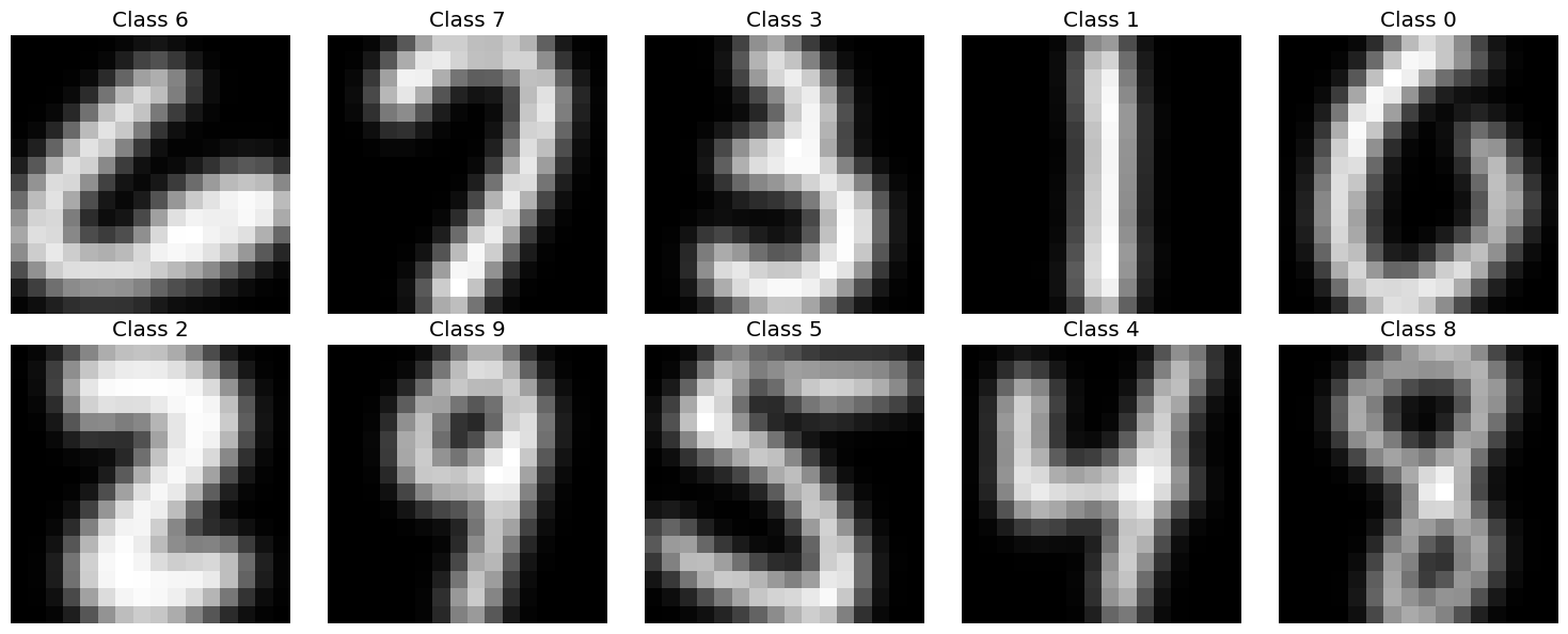
Figure 2: USPS image Direct Passing filter conversion to 16x16

Windowing and Pooling for Resolution Reduction: The input image $x$ undergoes a selective passing mechanism, where only the first pixel from every 2x2 window is retained. This operation can be mathematically represented as:

$$[x_{\text{reduced}}=\text{Resample}(x),$$ (5)

where $x_{\text{reduced}}$ represents the resolution-reduced image also shown in figure 2, and $\text{Resample}(x)$ is a function that selects every other pixel from the original image to achieve the desired down-sampling.

For instance, if the input image $x$ is of dimension $32\times 32$, this resolution reduction process reduces it to $16\times 16$.

4.3 Quantum VAE (Q-VAE) Encoder

The Quantum VAE (Q-VAE) integrates quantum computing into the encoding process, replacing the traditional classical neural network encoder with a quantum circuit as shown in Figure 1. The quantum encoder maps the input data into a quantum state representation, leveraging quantum superposition to capture complex relationships in the data. Quantum encoding enhances performance by converting the input into quantum states, enabling the Q-VAE to apply rotations to the data. The quantum-enhanced feature extraction is paired with a classical CNN decoder that reconstructs the input data, combining the strengths of quantum processing for feature extraction with classical techniques for data reconstruction.

The Q-VAE encoder compresses input data by encoding it into a lower-resolution latent space representation. It consists of a quantum circuit as shown in Figure 3, integrated with a classical fully connected layer.

The encoder transforms the input data $X$ into two key outputs: the mean $\mu$ and the log variance $\log(\sigma^{2})$ of the latent space distribution:

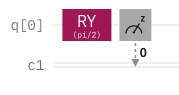
Figure 3: Quantum circuit for Quantum Variational Auto-encoder

The quantum encoding network, illustrated in Figure 2, uses a quantum encoding designed to process 16x16 pixel images that is the output of windowing pooling layer.

$$R_{Y}(x_{1})=\exp\left(-i\frac{x_{1}}{2}Y\right),$$ (6)

where $R_{Y}$ is the rotation gate around the $Y$-axis. The rotation gate $R_{Y}(\theta)$ can be expressed in terms of sine and cosine as:

$$R_{Y}(\theta)=\exp\left(-i\frac{\theta}{2}Y\right)=\cos\left(\frac{\theta}{2}\right)I-i\sin\left(\frac{\theta}{2}\right)Y$$ (7)

where $I$ is the identity matrix and $Y$ is the Pauli $Y$-matrix. The explicit matrix form is:

$$R_{Y}(\theta)=\begin{pmatrix}\cos\left(\frac{\theta}{2}\right)&-\sin\left(\frac{\theta}{2}\right)\\ \sin\left(\frac{\theta}{2}\right)&\cos\left(\frac{\theta}{2}\right)\end{pmatrix}$$ (8)

For the rotation gate applied to the first pixel, $R_{Y}(x_{1})$ becomes:

$$R_{Y}(x_{1})=\begin{pmatrix}\cos\left(\frac{x_{1}}{2}\right)&-\sin\left(\frac{x_{1}}{2}\right)\\ \sin\left(\frac{x_{1}}{2}\right)&\cos\left(\frac{x_{1}}{2}\right)\end{pmatrix}$$ (9)

The Pauli-$Z$ operator is applied to measure the quantum state and extract the latent variables $z$. The Pauli-$Z$ measurement flips the qubit’s state depending on the computational basis, effectively capturing the binary features of the image as shown in Figure 4.

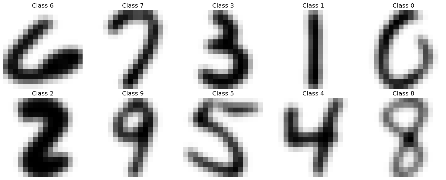
Figure 4: USPS Image resolution reduction from Quantum Circuit

Mathematically, the Pauli-$Z$ operator acts on the quantum state $\left|\psi\right\rangle$ as follows:

$$Z\left|0\right\rangle=\left|0\right\rangle,\quad Z\left|1\right\rangle=-\left|1\right\rangle$$ (10)

where $Z$ flips the phase of the qubit in the $\left|1\right\rangle$ state, while leaving the $\left|0\right\rangle$ state unchanged. This operation effectively translates quantum information into meaningful latent variables for the model. The resulting latent variables $z$ are given by:

$$z=\text{Measurement}(\left|\psi\right\rangle,Z)$$ (11)

After the quantum circuit processes the input image and extracts quantum features, the output of the quantum circuit, as shown in figure 4, is passed to fully connected layer. This transition enables the integration of quantum-encoded features with classical deep learning architectures. The quantum circuit produces an output, typically in the form of a reduced-resolution feature map or a vector. Let the output from the quantum circuit be denoted as $q_{\text{out}}$, where:

$$q_{\text{out}}=\text{QuantumCircuit}(x)$$ (12)

Here, $x$ is the input image, and $q_{\text{out}}$ represents the quantum-enhanced feature representation. The resolutionity of $q_{\text{out}}$ corresponds to the number of measurements or qubits used in the quantum circuit.

4.4 Shared Decoder Architecture

Despite the differences in their encoding mechanisms, all three models, C-VAE, CDP-VAE and Q-VAE share a common decoder architecture. This decoder is responsible for reconstructing the input data from the latent space representation. The decoder begins by transforming the latent variable \( z \) into a medium-resolution space through fully connected layers. Then, a series of transposed convolution (de-convolution) layers are used to progressively up-sample the data, restoring the original spatial dimensions. Finally, the output is passed through a sigmoid activation function to ensure that the pixel values are within the valid range (e.g,, between 0 and 1 for image data). This shared decoder allows for a fair comparison of the encoding techniques, with the focus on how the different encoders influence the quality of the reconstructed image.

5 Numerical Simulation

To assess the performance of our proposed model, we first need to preprocess the input image data. The preprocessing steps are as follows:

5.1 MNIST Dataset Pre-Processing

We utilized MNIST to determine whether the performance improvements observed in USPS could be replicated with MNIST. To enhance the model’s ability to generalize across different image sizes, we perform the following preprocessing steps also shown in Figure 5:

1. Cropping: Initially, the center of each image is cropped to remove any surrounding whitespace, reducing the image size from $28\times 28$ pixels to a smaller region that more tightly focuses on the handwritten digit (important features). The cropping ensures that the model receives more relevant features of the digits.

2. Resizing to $16\times 16$: After cropping, the image is resized to $16\times 16$ pixels. This step reduces the image resolution, making it easier for the model to process while still retaining key features of the digit. This process will help us to get same resolution dataset like USPS to see if MNIST also show improvement or not.

3. Resizing to $32\times 32$: Finally, the image is resized to $32\times 32$ pixels. This larger size is used for feeding the images into the neural network model, which is optimized to process medium resolution images. This resizing allows the model to capture finer details of the digits, enhancing its ability to reconstruct and classify the images effectively[16].

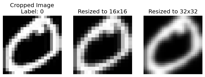
(a)

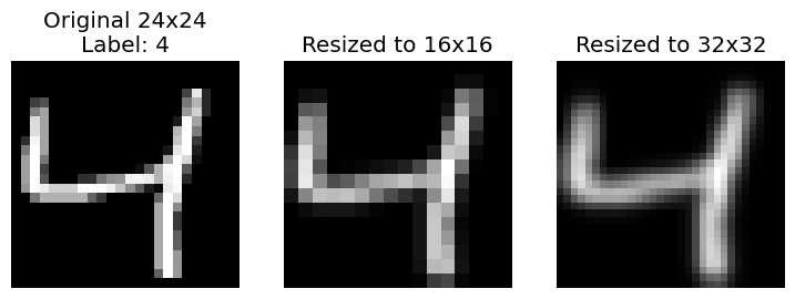
(b)

Figure 5: MNIST Image cropped for digit then transformed to 16x16 to 32x32.

This resizing step ensures compatibility with the input size of the model while retaining the features necessary for effective representation learning.

5.2 USPS Dataset Pre-Processing

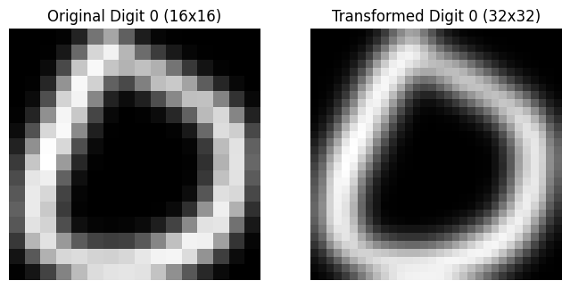
(a)

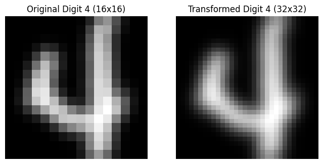
(b)

Figure 6: USPS Image transformed from 16x16 to 32x32.

USPS dataset has an image size 16x16. The interpolation method used during resizing adjusts the pixel values to fit the larger image grid, enabling the model to be tested with standard image input sizes, such as 32x32. USPS image conversion is shown in Figure 6.

5.3 Experimental Setup

In this section, we describe the hyper-parameters and settings used for training the models. We are implementing our algorithm on the Pennylane quantum simulator. Hyper-parameters to run the algorithm were carefully selected to ensure stable training while optimizing performance for all the models.

5.3.1 Hyper-parameters

In our training process, several key hyper-parameters were used to ensure efficient learning and model convergence. The learning rate was set to $0.001$ for all the models. This learning rate controls how much the model’s weights are updated in response to the computed gradients, providing a stable training process while allowing sufficient progress over the course of the training. The models were trained for 200 epochs, with each epoch representing one full pass of the data set through the model. This duration was chosen to ensure that the models had enough time to learn the underlying features of the data, while regular monitoring of the validation loss helped prevent over-fitting. A batch size of $400$ was used, which means that $400$ images were processed together before updating the model parameters. This batch size was selected to balance computational efficiency and the stability of gradient estimation, helping smooth gradient updates and ensuring more stable training. For optimization, we used the Adam optimizer, which is known for its adaptive learning rate that adjusts based on the first and second moments of the gradients. The Adam optimizer is particularly effective for models with many parameters and large datasets. The loss function used was the Binary Cross-Entropy Loss (BCELoss), with the argument reduction = ’sum’, which ensures that the individual losses across all pixels are summed rather than averaged. This choice emphasizes the total error in the reconstruction of the images. To visualize the progress of the model over time, the variables were used to store a grid of reconstructed images at various epochs. These images allowed us to visually assess how well the models were reconstructing the images as training progressed. These configurations were chosen to ensure effective model training, allowing the models to learn from the data efficiently and perform well in both reconstruction and evaluation tasks.

6 FID and MSE Performance Evaluation and Discussion

To evaluate the performance of the proposed models, we used a combination of several key metrics: the Fréchet Inception Distance (FID) score[18], training and testing loss, and Mean Squared Error (MSE)[19].

Each of these metrics provides distinct insights into the model’s ability to generate better-quality images and generalize to new data: Fréchet Inception Distance (FID) Score measures the similarity between the distribution of real and generated images. A lower FID score indicates that the generated images are closer in distribution to the real images, reflecting higher image fidelity and quality. The FID score is particularly useful for assessing the realism of generated images in generative models. Mean Squared Error (MSE) measures the average squared difference between the generated and real images. A lower MSE indicates that the generated images are closer to the real images in terms of pixel-wise accuracy. This metric is commonly used to evaluate the reconstruction quality in generative models, with lower values indicating better performance. By combining these metrics, we gain a comprehensive understanding of how well our models perform in terms of both image quality and generalizability.

The FID score was computed for 1) images reconstructed from the input images and 2) images generated from random noise, giving us insight into how well the models perform in generating realistic images from these two different sources of input.

The results are shown in table 1 below:

Table 1: Experimental Results

Datasets	FID Score for Image Reconstruction	FID Score for Image Generation	MSE
C-MNIST	40.7	94.4	0.0093
CDP-MNIST	39.7	93.3	0.0092
Q-MNIST	37.3	78.7	0.0088
C-USPS	50.4	73.1	0.0070
CDP-USPS	42.9	66.1	0.0065
Q-USPS	38.5	57.6	0.0058

The performance of all the models on the MNIST dataset was assessed by calculating the FID score using latent space representations as shown in Figure 7:

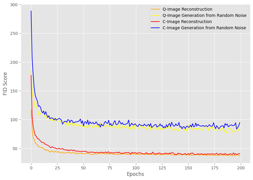
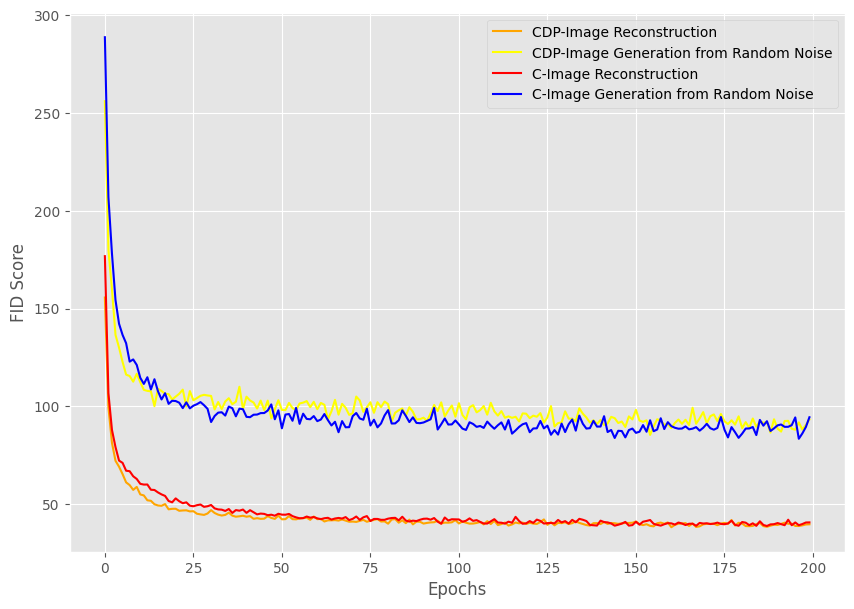
Figure 7: (a) MNIST FID Score for Quantum Variational Auto-encoder and (b) MNIST Direct Passing FID Score for Variational Auto-encoder.

For MNIST, the C-VAE achieves an FID score of 40.7 , indicating a reasonable ability to reconstruct images. CDP-VAE, demonstrates a slight improvement over the C-VAE with an FID score of 39.7 and then to Q-VAE, further improving upon CDP-VAE. The Q-VAE leverages quantum gates such as RY rotations to encode the data into a quantum state and Pauli-Z measurements bring quantum state to classical data, achieving a superior FID score of 37.3. This improved score suggests that the quantum model produces more faithful image reconstructions, capturing complex relationships in the data more effectively than the classical model. Although CDP-VAE approach is less complex, it still lacks the advanced feature extraction capabilities of the Q-VAE, which ultimately leads to lower reconstruction fidelity.

For the USPS dataset, the Q-VAE achieved an impressive FID score of 57.6, indicating better-quality image reconstructions and strong performance in terms of both fidelity and distribution similarity to the original dataset. This result highlights the effectiveness of the Q-VAE in handling simpler grayscale datasets, where it demonstrates superior feature extraction and reconstruction capabilities.

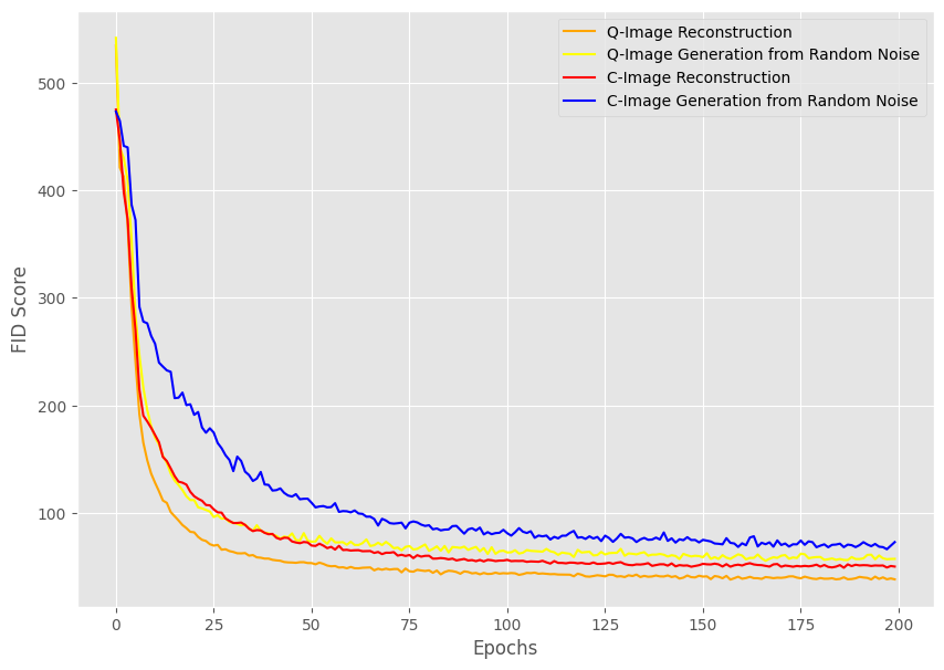
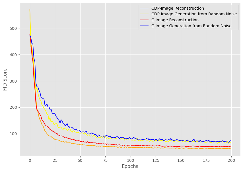
Figure 8: (a) USPS FID Score for Variational Quantum Auto encoder and (b) USPS Direct Passing FID Score for Variational Auto encoder.

Despite its simplicity, the CDP-VAE still achieved relatively good performance on the USPS dataset, with an FID score of 66.1 as shown in Figure 8.

On the MNIST dataset, C-VAE, with an MSE of 0.0093, showed slightly higher error compared to the Q-VAE, indicating that while it performs well, its feature extraction capabilities are not as advanced as those of the quantum model. Despite its relatively low MSE, the classical model’s performance is constrained by the limitations of traditional neural network-based encoding and decoding methods, which cannot capture the full complexity of the data as efficiently as quantum circuits. The CDP-VAE, with an MSE of 0.0092, performs little better then C-VAE While Q-VAE achieved the lowest MSE of 0.0088, demonstrating its ability to produce high-fidelity reconstructions compared to the other models. This is consistent with the Q-VAE’s superior performance across other metrics such as training and testing loss. The quantum-based encoding method enables the Q-VAE to extract richer feature representations, leading to more accurate reconstructions. The quantum model’s ability to capture complex dependencies between pixels allows it to outperform classical approaches, even when dealing with highly structured images like those in the MNIST dataset.

6.1 Reconstructed Images:

Figure 9 displays reconstructed grayscale digit images from the MNIST dataset, arranged in a grid format. The input image is first downscaled from 28x28 to 16x16, and then upscaled to 32x32. This sequence reveals that some images lose details during resolution reduction, leading to inaccuracies in their reconstruction. For example, the digit ’3’ in the 4th row and 1st column is successfully reconstructed by the Quantum VAE (Q-VAE), whereas the Classical VAE (C-VAE) and Direct Passing VAE (CDP-VAE) struggle to generate a well-defined version. However, in the 5th row and 3rd column, the digit ’0’ shows noticeable noise due to the resolution reduction, making it difficult to reconstruct accurately. In this case, C-VAE incorrectly generates a ’7’, while Q-VAE produces a hybrid image that blends ’7’ and ’0’. Most digits retain their recognizable shapes, but some exhibit blurriness or distortions as column 3, row 5 and ’6’ its difficult to recognise the image as ’7’ and ’9’, indicating challenges in capturing finer details during the reconstruction process. These issues may stem from factors such as limited latent space resolution’s used for the model (i.e 16), preprocessing steps like resizing or normalization, or suboptimal model architecture. Interestingly, prior evaluations using metrics like the FID have demonstrated that quantum-based approaches, particularly Quantum Variational Autoencoders (Q-VAE), achieve superior image quality on MNIST. The observed FID scores confirm that quantum-enhanced and hybrid methods produce sharper and more detailed reconstructions compared to classical models.

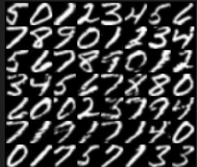
(a) Input Image

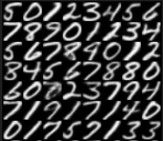
(b) C-VAE

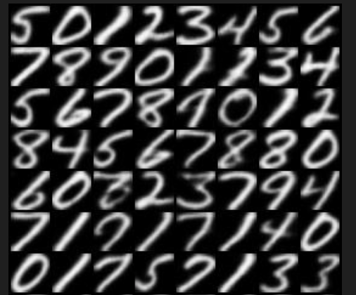
(c) CDP-VAE

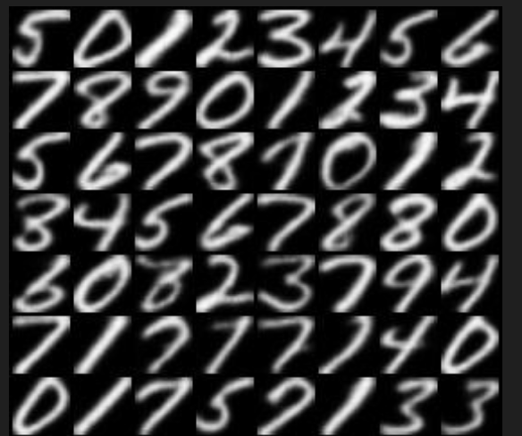
(d) Q-VAE

Figure 9: Comparing Classical and Quantum Reconstructed Images. (a) MNIST Input First Down-sampled from 28x28 to 16x16 then Up-sampled Image from 16x16 to 32x32 resolution (b) Classical VAE Image Reconstructions, (c) MNIST CDP-VAE reconstructed images and (d) MNIST Q-VAE reconstructed images for Variational Autoencoder.

USPS images reconstructed from 3 different VAE models have been shown in Figure 10.

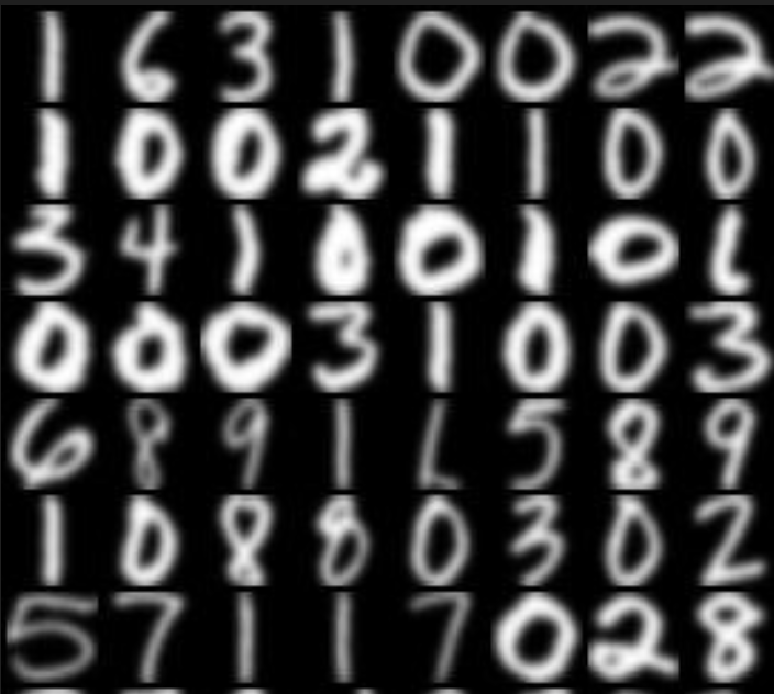
(a) Input Image

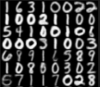
(b) C-VAE

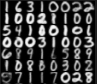
(c) CDP-VAE

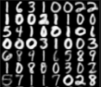
(d) Q-VAE

Figure 10: Comparing Classical and Quantum Reconstructed Images. (a) USPS Input Up-sampled Image from 16x16 to 32x32 resolution (b) Classical VAE Image Reconstructions, (c) USPS CDP-VAE reconstructed images and (d) USPS Q-VAE reconstructed images for Variational Autoencoder.

While this score indicates that the model can generate images with reasonable fidelity (i.e., the generated images resemble real USPS digits), it lags behind the performance of the Q-VAE. The quantum model’s ability to leverage more complex transformations in the latent space for image reconstruction enables it to capture more intricate patterns and feature representations in the data. This allows the Q-VAE to achieve lower FID scores (indicating higher image fidelity) compared to the CDP-VAE and C-VAE as seen in the results for the USPS dataset. For MSE, the Q-VAE again outperformed the other models, achieving a score of 0.0058. This lower error indicates that the quantum model is particularly effective at capturing the more complex, medium-resolution patterns in the USPS images. The Q-VAE’s quantum-enhanced encoding allows it to extract intricate features from the grayscale images, leading to more accurate reconstructions. Its performance on USPS highlights the potential of quantum circuits in improving image generation tasks, especially for datasets with more complex structures compared to MNIST. The C-VAE, with an MSE of 0.0070, performed worse than the Q-VAE and CDP-VAE on USPS, reflecting the same trend observed in MNIST. While still a competitive model, the C-VAE’s ability to reconstruct images is limited by its classical encoding mechanism. The model performs well, but its lack of advanced feature extraction techniques prevents it from achieving the same reconstruction quality as the Q-VAE. The CDP-VAE with an MSE of 0.0065, performance is better than the C-VAE on MNIST, it still lags behind both the Q-VAE on USPS. While reconstructed images we can see Q-VAE is reconstructing very well competing with C-VAE and CDP-VAE.

6.2 New Generated Images:

The performance of the three models in handling random noise varies considerably. The generated images presented were captured at epoch 200. The Classical VAE requires more time to converge, necessitating longer training. Therefore, we evaluate the model at epoch 200 to assess its performance after sufficient training. While initial epochs Q-VAE has shown fast convergence at epoch 20, while other models were unable to generate digits even at epoch 20 .The Q-VAE outperforms the other models, achieving an FID score of 78.7 at epoch 200. This suggests that the Q-VAE is more resilient to noise, as it is capable of generating better-quality images even when starting from random noise inputs. In contrast, the C-VAE struggles with random noise, resulting in a much higher FID score of 94.4, indicating poor performance in reconstructing images from noisy inputs. The CDP-VAE also faces challenges with noise but performs slightly better than the C-VAE, with an FID score of 93.3. While both the C-VAE and CDP-VAE show limitations in noise handling, the Q-VAE demonstrates a notable advantage in generating more realistic images in the presence of noise. MNIST generated images from noise, have been shown below in Figure 11:

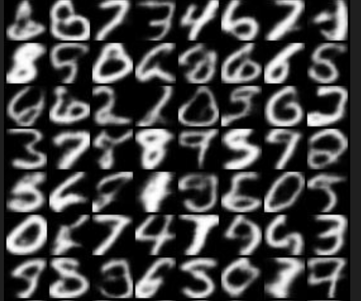
(a) C-VAE MNIST New Generated Images

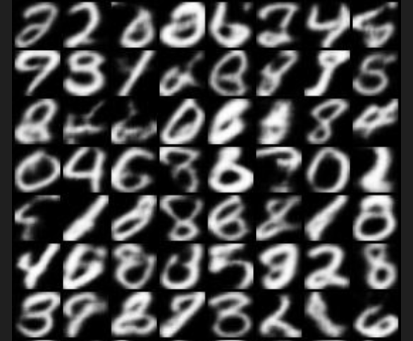
(b) CDP-VAE New Generated Images

(c) Q-VAE New Generated Images

Figure 11: MNIST New Generated Images from Random Noise

Figure 11 shows newly generated grayscale digit images, likely synthesized from random noise using VAE. These images are organized in a grid format, with varying levels of clarity and detail. While some digits are clearly defined and resemble their expected shapes, others appear blurry, distorted, or lack fine structural details, indicating limitations in the model’s ability to fully capture the underlying data distribution. These artifacts could result from constraints such as an insufficiently expressive latent space, challenges in training stability, or limitations in the model architecture. For instance, models with lower-resolution latent spaces may struggle to encode the nuanced variations required to generate sharp, realistic images.

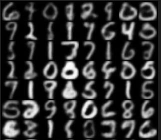
(a) C-VAE USPS New Generated Images

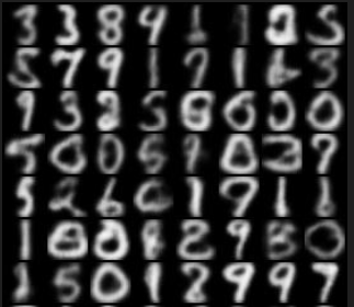
(b) CDP-VAE New Generated Images

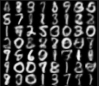
(c) Q-VAE New Generated Images

Figure 12: USPS New Generated Images from Random Noise

Interestingly, Q-VAE have demonstrated better performance in similar tasks, as reflected in improved FID scores. Q-VAE, in particular, have shown a remarkable ability to generate better-quality images from noise These operations are highly effective at capturing complex patterns and correlations in medium-resolution data, enabling more detailed and coherent outputs. Figure 12 shows how well Quantum can generate new images from noise while using only quantum superposition. The quantum advantage enables the model to effectively capture complex patterns from random noise, producing high-quality, leading to more realistic images [17] This highlights the advantage of quantum-based encoding in generating better-quality images, particularly in tasks that require nuanced and medium-resolution data representations, such as image reconstruction or generation.

6.2.1 Trainable Parameters

The results indicates that our proposed model Q-VAE and its similar approach in classical, CDP-VAE, both have shown significant improvement over C-VAE architectures in terms of parameter efficiency. Specifically, the C-VAE has a total of 407,377 trainable parameters, with 299,424 parameters dedicated to the encoder and 107,953 parameters assigned to the decoder. In contrast, the Quantum VAE significantly reduces the number of trainable parameters, totaling only 144,977 parameters. This is achieved by the quantum model’s more compact encoder, which contains only 37,024 parameters, a dramatic reduction compared to the classical VAE. This reduction highlights the efficiency of the quantum approach in learning and representing complex features with a smaller number of parameters, enabling better latent space compression.

Despite this reduction in parameters, the decoder structure remains similar between the quantum and classical models, both utilizing 107,953 parameters. This consistency in the decoder ensures that the Quantum VAE maintains comparable image reconstruction capabilities to the classical model, while benefiting from the quantum encoder’s enhanced efficiency. The lower parameter count in the QVAE encoder illustrates the potential of quantum circuits to offer a more resource-efficient alternative for training and generating better-quality image reconstructions. These findings underscore the practical benefits of quantum computing in optimizing VAE architectures, especially in tasks that require high-fidelity image generation and accurate reconstruction. While classical VAEs remain a strong choice for many machine learning applications, the Q-VAE shows promising advancements, particularly in fields where image quality and computational efficiency are paramount. Potential applications of quantum VAEs include digital imaging, healthcare diagnostics, and creative arts, where high-quality image generation is critical. However, despite these advantages, the adoption and effectiveness of Q-VAE still face challenges, including issues related to the scalability of quantum hardware and the complexity of quantum algorithms. Continued research and development in quantum machine learning are essential for unlocking the full potential of quantum-enhanced models, pushing the boundaries of what is achievable in generative modeling and real-world applications.

7 Conclusion

In this study, we introduce the Quantum Down-sampling Filter for Variational Auto-encoder (Q-VAE), a novel model that integrates quantum computing into the encoder component of a traditional VAE. Our experimental results demonstrate that Q-VAE offers significant advantages over classical VAE architectures across various performance metrics. In particular, Q-VAE consistently outperforms classical VAE, achieving lower FID scores, indicating superior image fidelity and the ability to generate better-quality reconstructions. The quantum-enhanced encoder captures more intricate features of the images, leading to improved generative performance. We evaluated the model on digit datasets such as MNIST and USPS, initially up-scaled to 32x32 for consistency. For a fair comparison, we also tested our quantum-enhanced model alongside a classical counterpart and a model mimicking classical behavior, referred to as Classical Direct Passing (CDP-VAE). One more key finding of this study is the significant reduction in the number of trainable parameters in the Q-VAE’s and CDP-VAE’s encoder. With only 37,024 parameters, the Q-VAE dramatically reduces computational complexity compared to the classical VAE, which contains over 407,000 trainable parameters. This reduction highlights the efficiency of quantum-based encoding methods, which offers the potential for more scalable and resource-efficient models. The results highlight the practical advantages of incorporating quantum computing into VAEs, particularly for tasks that require high-quality image generation and feature extraction. The Q-VAE not only improves image quality, but also enhances computational efficiency, making it a promising candidate for future applications in areas such as computer vision, data synthesis, and beyond. These findings suggest that further exploration of quantum-enhanced machine learning techniques could unlock new possibilities in generative modeling and image reconstruction, offering both performance improvements and computational savings.

References

- [1] L. Pinheiro Cinelli, M. Araújo Marins, E. A. Barros da Silva, and S. Lima Netto, "Variational Autoencoder," in Variational Methods for Machine Learning with Applications to Deep Networks, Springer International Publishing, 2021, pp. 111–149.
- [2] B. Everett, An Introduction to Latent Variable Models, Springer Science & Business Media, 2013.
- [3] S. H. Khan, M. Hayat, and N. Barnes, "Adversarial Training of Variational Auto-Encoders for High Fidelity Image Generation," in 2018 IEEE Winter Conference on Applications of Computer Vision (WACV), IEEE, 2018, pp. 1312–1320.
- [4] D. P. Kingma and M. Welling, "An introduction to variational autoencoders," Foundations and Trends® in Machine Learning, vol. 12, no. 4, pp. 307
- [5] C. Andrews, A. Endert, B. Yost, and C. North, "Information Visualization on Large, High-Resolution Displays: Issues, Challenges, and Opportunities," Information Visualization, vol. 10, no. 4, pp. 341–355, 2011.
- [6] J. Tian, X. Sun, Y. Du, S. Zhao, Q. Liu, K. Zhang, and D. Tao, "Recent Advances for Quantum Neural Networks in Generative Learning," IEEE Transactions on Pattern Analysis and Machine Intelligence, vol. 45, no. 10, pp. 12321–12340, 2023.
- [7] S. Ahmed, C. Sánchez Muñoz, F. Nori, and A. F. Kockum, "Classification and Reconstruction of Optical Quantum States with Deep Neural Networks," Physical Review Research, vol. 3, no. 3, pp. 033278, 2021.
- [8] G. Gonçalves, "A Comparative Study of Data Augmentation Techniques for Image Classification: Generative Models vs. Classical Transformations," M.S. thesis, Universidade de Aveiro, 2020.
- [9] O. Laousy, "Deep Learning Methods for Localization, Segmentation, and Robustness in Medical Imaging," Ph.D. thesis, Université Paris-Saclay, 2024.
- [10] D. E. Diamantis, P. Gatoula, A. Koulaouzidis, and D. K. Iakovidis, "This Intestine Does Not Exist: Multiscale Residual Variational Autoencoder for Realistic Wireless Capsule Endoscopy Image Generation," IEEE Access, vol. 12, pp. 25668–25683, 2024.
- [11] L. Brigato, B. Barz, L. Iocchi, and J. Denzler, "Image Classification with Small Datasets: Overview and Benchmark," IEEE Access, vol. 10, pp. 49233–49250, 2022.
- [12] S. V. Armstrong, S. Pallickara, S. Ghosh, and J. F. Breidt, "Transformer, Diffusion, and GAN-Based Augmentations for Contrastive Learning of Visual Representations," 2024.
- [13] J. R. Hershey and P. A. Olsen, "Approximating the Kullback-Leibler Divergence Between Gaussian Mixture Models," in 2007 IEEE International Conference on Acoustics, Speech and Signal Processing (ICASSP’07), IEEE, vol. 4, pp. IV-317, 2007.
- [14] T. Hu, F. Chen, H. Wang, J. Li, W. Wang, J. Sun, and Z. Li, "Complexity Matters: Rethinking the Latent Space for Generative Modeling," Advances in Neural Information Processing Systems, vol. 36, 2024.
- [15] M. Schuld and N. Killoran, "Quantum Machine Learning in Feature Hilbert Spaces," Physical Review Letters, vol. 122, no. 4, pp. 040504, 2019.
- [16] D. Duarte, F. Nex, N. Kerle, and G. Vosselman, "Multi-resolution feature fusion for image classification of building damages with convolutional neural networks," Remote Sensing, vol. 10, no. 10, pp. 1636, 2018.
- [17] Y. Altmann, S. McLaughlin, M. J. Padgett, V. K. Goyal, A. O. Hero, and D. Faccio, "Quantum-inspired computational imaging," Science, vol. 361, no. 6403, pp. eaat2298, 2018.
- [18] Y. Yu, W. Zhang, and Y. Deng, "Frechet Inception Distance (FID) for Evaluating GANs," China University of Mining Technology Beijing Graduate School, vol. 3, 2021.
- [19] T. O. Hodson, T. M. Over, and S. S. Foks, "Deconstructing mean squared error," Journal of Advances in Modeling Earth Systems, vol. 13, no. 12, pp. e2021MS002681, 2021.
- [20] S. R. Shah and M. Vatsa, "Enhancing Quantum Diffusion Models with Pairwise Bell State Entanglement," in Proceedings of the International Conference on Pattern Recognition, pp. 347-361, Springer, Cham, 2025.
- [21] J. Tomczak and M. Welling, "VAE with a VampPrior," in International Conference on Artificial Intelligence and Statistics, PMLR, 2018, pp. 1214–1223.
- [22] J. Peng, D. Liu, S. Xu, and H. Li, "Generating diverse structure for image inpainting with hierarchical VQ-VAE," in Proceedings of the IEEE/CVF Conference on Computer Vision and Pattern Recognition, 2021, pp. 10775–10784.
- [23] A. Razavi, A. Van den Oord, and O. Vinyals, "Generating diverse high-fidelity images with VQ-VAE-2," in Advances in Neural Information Processing Systems, vol. 32, 2019.
- [24] T. Bepler, E. Zhong, K. Kelley, E. Brignole, and B. Berger, "Explicitly disentangling image content from translation and rotation with spatial-VAE," in Advances in Neural Information Processing Systems, vol. 32, 2019.
- [25] H. W. L. Mak, R. Han, and H. H. Yin, "Application of variational autoencoder (VAE) model and image processing approaches in game design," Sensors, vol. 23, no. 7, pp. 3457, 2023.
- [26] A. A. Neloy and M. Turgeon, "A comprehensive study of auto-encoders for anomaly detection: Efficiency and trade-offs," Machine Learning with Applications, vol. 100572, 2024.
- [27] M. Elbattah, C. Loughnane, J. L. Guérin, R. Carette, F. Cilia, and G. Dequen, "Variational autoencoder for image-based augmentation of eye-tracking data," Journal of Imaging, vol. 7, no. 5, pp. 83, 2021.
- [28] I. Gatopoulos, M. Stol, and J. M. Tomczak, "Super-resolution variational auto-encoders," arXiv preprint arXiv:2006.05218, 2020.
- [29] Y. Wang, D. Li, L. Li, R. Sun, and S. Wang, "A novel deep learning framework for rolling bearing fault diagnosis enhancement using VAE-augmented CNN model," Heliyon, vol. 10, no. 15, 2024.
- [30] B. Dai and D. Wipf, "Diagnosing and enhancing VAE models," arXiv preprint arXiv:1903.05789, 2019.
- [31] X. Hou, L. Shen, K. Sun, and G. Qiu, "Deep feature consistent variational autoencoder," in 2017 IEEE Winter Conference on Applications of Computer Vision (WACV), pp. 1133–1141, 2017. DOI: https://doi.org/10.1109/WACV.2017.00134.
- [32] Z. Yang, Z. Hu, R. Salakhutdinov, and T. Berg-Kirkpatrick, "Improved variational autoencoders for text modeling using dilated convolutions," in International Conference on Machine Learning (ICML), PMLR, vol. 70, pp. 3881–3890, 2017.
- [33] A. Makhzani, J. Shlens, N. Jaitly, I. Goodfellow, and B. Frey, "Adversarial autoencoders," arXiv preprint arXiv:1511.05644, 2015.
- [34] J. Kos, I. Fischer, and D. Song, "Adversarial examples for generative models," in 2018 IEEE Security and Privacy Workshops (SPW), pp. 36–42, 2018.
- [35] S. Sinha, S. Ebrahimi, and T. Darrell, "Variational adversarial active learning," in Proceedings of the IEEE/CVF International Conference on Computer Vision, pp. 5972–5981, 2019.
- [36] M. Cheng, F. Fang, C. C. Pain, and I. M. Navon, "An advanced hybrid deep adversarial autoencoder for parameterized nonlinear fluid flow modelling," Computer Methods in Applied Mechanics and Engineering, vol. 372, pp. 113375, 2020.
- [37] A. Jabbar, X. Li, and B. Omar, "A survey on generative adversarial networks: Variants, applications, and training," ACM Computing Surveys (CSUR), vol. 54, no. 8, pp. 1–49, 2021.
- [38] A. Khoshaman, W. Vinci, B. Denis, E. Andriyash, H. Sadeghi, and M. H. Amin, "Quantum variational autoencoder," Quantum Science and Technology, vol. 4, no. 1, pp. 014001, 2018.
- [39] O. Ambacher, J. Majewski, C. Miskys, A. Link, M. Hermann, and M. Eickhoff, "Pyroelectric properties of Al (In) GaN/GaN hetero- and quantum well structures," Journal of Physics: Condensed Matter, vol. 14, no. 13, pp. 3399, 2002.
- [40] A. Rocchetto, E. Grant, S. Strelchuk, G. Carleo, and S. Severini, "Learning hard quantum distributions with variational autoencoders," npj Quantum Information, vol. 4, no. 1, pp. 28, 2018.
- [41] N. Gao, M. Wilson, T. Vandal, W. Vinci, R. Nemani, and E. Rieffel, "High-dimensional similarity search with quantum-assisted variational autoencoder," in Proceedings of the 26th ACM SIGKDD International Conference on Knowledge Discovery and Data Mining, pp. 956–964, 2020.
- [42] A. I. Gircha, A. S. Boev, K. Avchaciov, P. O. Fedichev, and A. K. Fedorov, "Training a discrete variational autoencoder for generative chemistry and drug design on a quantum annealer," arXiv preprint arXiv:2108.11644, 2021.
- [43] G. Wang, J. Warrell, P. S. Emani, and M. Gerstein, "-QVAE: A Quantum Variational Autoencoder utilizing Regularized Mixed-state Latent Representations," arXiv preprint arXiv:2402.17749, 2024.
- [44] I. A. Luchnikov, A. Ryzhov, P. J. Stas, S. N. Filippov, and H. Ouerdane, "Variational autoencoder reconstruction of complex many-body physics," Entropy, vol. 21, no. 11, pp. 1091, 2019.
- [45] M. Bhupati, A. Mall, A. Kumar, and P. K. Jha, "Deep Learning-Based Variational Autoencoder for Classification of Quantum and Classical States of Light," Adv. Phys. Res., vol. 2024, pp. 2400089, 2024.