Scalable Cosmic AI Inference using Cloud Serverless Computing with FMI

Abstract

Large-scale astronomical image data processing and prediction is essential for astronomers, providing crucial insights into celestial objects, the universe’s history, and its evolution. While modern deep learning models offer high predictive accuracy, they often demand substantial computational resources, making them resource-intensive and limiting accessibility. We introduce the Cloud-based Astronomy Inference (CAI) framework to address these challenges. This scalable solution integrates pre-trained foundation models with serverless cloud infrastructure through a Function-as-a-Service (FaaS) Message Interface (FMI). CAI enables efficient and scalable inference on astronomical images without extensive hardware. Using a foundation model for redshift prediction as a case study, our extensive experiments cover user devices, HPC (High-Performance Computing) servers, and Cloud. CAI’s significant scalability improvement on large data sizes provides an accessible and effective tool for the astronomy community. The code is accessible at https://github.com/UVA-MLSys/AI-for-Astronomy.

1 Introduction

Astronomical images are vital to modern astrophysics, offering key insights into celestial objects, such as their shape Willett et al. (2013), distance Hubble (1929), and other fundamental characteristics that define our understanding of the universe. Large surveys like the Dark Energy Spectroscopic Instrument (DESI) Fan et al. (2019) and the Sloan Digital Sky Survey (SDSS) Gunn et al. (1998) provide extensive image datasets with unique attributes. For example, SDSS images consist of five spectral bands—u, g, r, i, and z—each focused on specific wavelengths: Ultraviolet (u) at 3543 Å, Green (g) at 4770 Å, Red (r) at 6231 Å, Near Infrared (i) at 7625 Å, and Infrared (z) at 9134 Å Murrugarra-Llerena and Hirata (2017).

Deep learning foundation models trained on large-scale astronomical image datasets have proven to be powerful tools for improving the accuracy and efficiency of tasks such as redshift prediction, morphology classification, and similarity search Hayat et al. (2021); Lanusse et al. (2023); Fathkouhi and Fox (2024). Figure 5 highlights several notable deep-learning architectures that leverage astronomical images for prediction. For example, AstroCLIP Lanusse et al. (2023) uses an image transformer with a 307M-parameter encoder, pretrained on approximately 197K images. AstroMAE Fathkouhi and Fox (2024) combines frozen pretrained weights with fine-tunable parameters, totaling 10.4M learnable parameters. Similarly, Henghes et al. (2022) trained their model on 1 million SDSS images using 7.8M parameters. In comparison, AstroMAE, trained on about 650K images, showed significant performance improvements over the Henghes et al. (2022) model in redshift prediction.

While these models yield impressive results, their large parameter counts require substantial computational resources, making both training and inference resource-intensive. The memory and computing resources on a standalone device become a limitation for users to run on large datasets and foundation models. There is a need for advanced infrastructure to overcome the limit of high-performance inference accessibility for many users Neely (2021). Serverless computing is a recently popular Function-as-a-Service (FaaS) Li et al. (2022), that lets developers write cloud functions in high-level languages (e.g. Python) and takes care of the complex infrastructure management itself.

This study proposes a highly scalable serverless computing framework for using AWS AWS (2024) to enhance the accessibility of a pretrained foundation model for astronomical images. This effectively reduces the computational demands on individual users. In summary, we offer the following contributions:

• A novel Cloud-based Astronomy framework (named “Cloud-based Astronomy Inference” (CAI)) to significantly enhance the scalability of foundation model inference on large astronomical images.

• Detailed experiments on the redshift prediction task using real-world galaxy images from the SDSS survey, comparing CAI’s performance with other computing devices (e.g. personal, and HPC).

• Our comprehensive performance analysis with inference time and throughput demonstrates that CAI effectively improves the scalability of foundation model inference in astronomy.

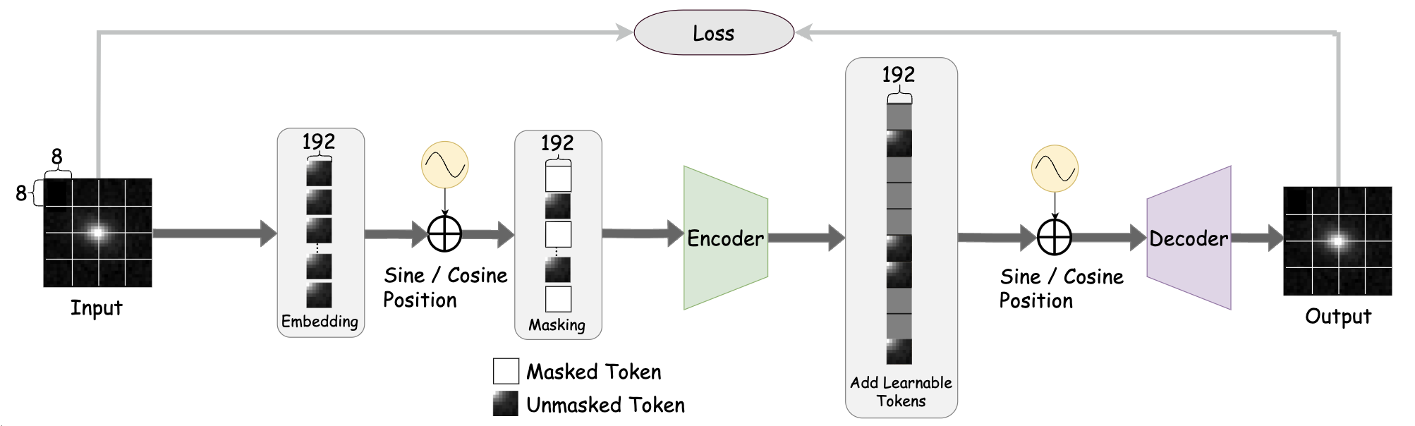
Figure 1: The architecture of masked autoencoder of AstroMAE Fathkouhi and Fox (2024).

2 Related Work

The immense size of astronomy datasets has made cloud services essential for efficiently storing and processing this data. Faaique (2024) highlighted the significant challenges such massive volumes pose, emphasizing cloud computing as a key solution to managing these issues. Kim and Hahm (2011) investigated requirements for cloud computing used by scientists dealing with the increasing size of big science datasets. Gill and Buyya (2020) accepted the invaluable nature of cloud computing for large astronomy datasets and used an astronomy case study to test their proposed cloud computing model that improves failure management. Khlamov et al. (2022) argued that cloud services are nearly indispensable for managing astronomy datasets, especially those dense in metadata and images. In their study on variable star photometry, they implemented a Software-as-a-Service (SaaS) model to effectively address the substantial storage demands.

De Prado et al. (2014) leveraged cloud computing for the Mosaic tool, enabling the rapid and efficient creation of sky mosaics from images captured across different sky regions. Zhang et al. (2020) implemented the distributed astronomy image processing toolkit called Kira by running Apache Spark on an Amazon EC2 cloud. Their speed-up results and throughput indicate that this parallelized computing method is compatible with astronomy applications. Sen et al. (2022) underscored the minimal scalability concerns of cloud services, noting the effectiveness of cloud-based distributed frameworks for tasks like redshift prediction. Furthermore, Parra-Royón et al. (2024) leveraged Function-as-a-Service (FaaS) models and decision-making systems to manage the computationally intensive processing of radio astronomy data.

These studies highlight the essential role of cloud services in overcoming the computational and storage challenges inherent in modern astronomical research. To our knowledge, no prior work has leveraged serverless computing AWS (2024) to enhance the scalability of foundation models for astronomical images.

3 Problem Statement

In astronomical imaging, much of the research has focused on enhancing deep learning model performance, with comparatively less attention to scaling inference capabilities. Although recent foundation models, trained on extensive astronomical image datasets, demonstrate versatility across various tasks, their high parameter count limits usability and scalability due to infrastructure constraints. To address this, a scalable framework is essential for efficient inference on large image volumes without added financial burdens. We introduce Cloud-based Astronomy Inference (CAI), which employs the Function-as-a-Service (FaaS) Message Interface (FMI) Böhringer (2022) to enhance the scalability of foundation models trained on astronomical images. Based on our review, CAI is the first framework specifically designed to address the inference scalability of foundation models in astronomical imaging.

Although dark energy constitutes approximately 95% of the universe’s energy, our understanding of this mysterious force remains profoundly limited. Investigating and exploring its nature requires a large-scale collection of galaxy images, supported by advanced cosmological methods and theories Jones et al. (2024). A cornerstone of these methods is the precise determination of a critical parameter: redshift. Redshift measures how much the light from a celestial object has been stretched, providing crucial insights into the distances of these objects and the expansion of the universe Hubble (1929).

In this study, we assess CAI’s scalability by applying it to redshift prediction. For this purpose, we selected AstroMAE due to its superior performance and because it is pretrained on a larger dataset, which may enhance generalization compared to AstroCLIP. Future work will explore the scalability of additional models discussed in this context.

4 Methodology

We first collect the AstroMAE model pretrained on the large astronomy dataset. Then deploy it to our proposed cloud architecture for inference scalability benchmark.

4.1 AstroMAE

AstroMAE Fathkouhi and Fox (2024) is a recent foundation model that captures general patterns in galaxy images for redshift prediction. It has two major phases:

4.1.1 Pretraining:

Figure 1 illustrates the pretraining process of AstroMAE’s masked autoencoder Devlin (2018). The masked autoencoder aims to reconstruct masked patches using unmasked ones. We mask 75% of the embedded patches, the remaining 25% are fed into the encoder. Initially, images are segmented into uniform patches of size 5×8×8 and embedded into 192-dimensional vectors with positional embedding.

The reconstructed masked patches are compared to their original patches, enabling the model to learn meaningful representations. To promote learning of data patterns instead of memorizing patch positions, the embeddings are randomly shuffled before being input to the encoder. Compared to other pretraining methods like contrastive learning Chen et al. (2020), the masked autoencoder does not rely on specific augmentations, which can potentially increase the dataset size and computational demands. In contrast, AstroMAE’s masked autoencoder processes 25% patches, making it significantly more efficient. A crucial step for working on large astronomy data. AstroMAE also uses a modified ViT Wang et al. (2022), that contains a parallel convolutional module and performs even better.

4.1.2 Fine-tuning:

During fine-tuning, the decoder is removed, leaving a frozen encoder that works with two additional models: a parallel Inception model and a magnitude block. The outputs from the frozen encoder, Inception model, and magnitude block are first processed through several layers individually, then concatenated and passed through additional layers for final processing.

Let $V\in R^{I}$ represent the image data and $O\in R^{M}$ represent the magnitude data, where $I$ and $M$ denote the dimensions of the image and magnitude data spaces, respectively.

A frozen pretrained encoder $E:{R}^{I}\rightarrow{R}^{C}$ generates a latent space representation $L_{E}$ from the image $V$:

$$L_{E}=E(V).$$ (1)

Similarly, an inception model $W:{R}^{I}\rightarrow{R}^{Q}$ extracts features $L_{W}$ from the same image of Figure 2a).

$$L_{W}=W(V).$$ (2)

The magnitude data $O$ from Figure 2b) is processed through a magnitude block $S:{R}^{M}\rightarrow{R}^{T}$, resulting in magnitude features $L_{T}$:

$$L_{T}=S(O).$$ (3)

To further process these image features, AstroMAE applies two fully connected layers with a ReLU activation in between to both $L_{E}$ and $L_{W}$. The resulting features are denoted as $L_{EC}$ and $L_{WC}$, representing the processed outputs of the frozen encoder and the inception model in Figure 2c), respectively.

$$L_{EC} =FC(\text{ReLU}(FC(L_{E}))),$$ (4)

$$L_{WC} =FC(\text{ReLU}(FC(L_{W}))).$$ (5)

Finally, the redshift prediction $P^{RS}$ is obtained as shown in Figure 2d) by concatenating $L_{T}$, $L_{EC}$, and $L_{WC}$, and then passing them through two fully connected layers with a ReLU activation function in between:

$$P^{RS}=FC(\text{ReLU}(FC(\text{Concat}(L_{T},L_{EC},L_{WC}))))$$ (6)

The predicted redshift $P^{RS}$ is compared with the actual redshift $R^{RS}$, and the cost is calculated using the Mean Squared Error (MSE) over $N$ samples:

$$\text{MSE}=\frac{1}{N}\sum_{i=1}^{N}\left(P^{RS}_{i}-R^{RS}_{i}\right)^{2}$$ (7)

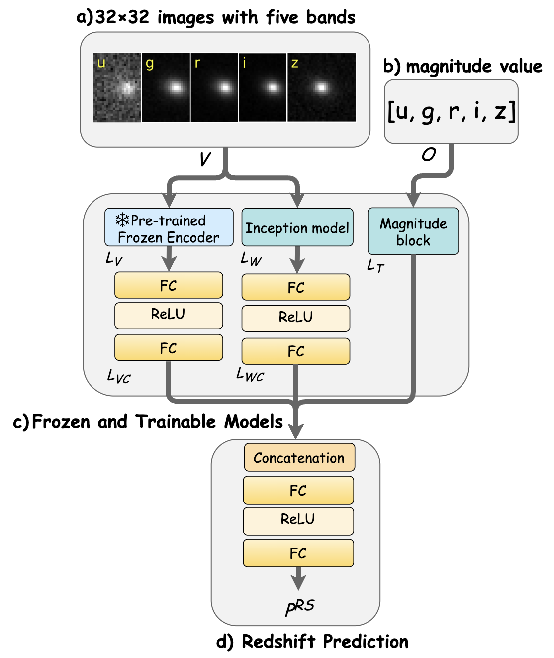
Figure 2: AstroMAE fine-tuning architecture.

Table 1: Redshift Prediction Using Various Architectures with AstroMAE Fathkouhi and Fox (2024).

Training Type	Architecture	MSE	MAE
Supervised Training (from scratch)	plain-ViT-magnitude	0.00077	0.01871
	pcm-ViT-magnitude	0.00057	0.01604
	Henghes et al. (2022)	0.00058	0.01568
	plain-ViT	0.00097	0.02123
	pcm-ViT	0.00063	0.01686
	Inception-only	0.00064	0.01705
Fine-Tuning	plain-ViT-magnitude	0.00068	0.01740
	pcm-ViT-magnitude	0.00060	0.01655
	plain-AstroMAE	0.00056	0.01558
	pcm-AstroMAE	0.00053	0.01520
	plain-ViT	0.00086	0.01970
	pcm-ViT	0.00084	0.01945
	plain-ViT-inception	0.00059	0.01622
	pcm-ViT-inception	0.00059	0.01601

Table 4.1.2 shows the performance of various architectures combining a pretrained encoder, magnitude block, and the inception model. Rows labeled “from-scratch” denote models where both plain-ViT Dosovitskiy (2020) and pcm-ViT Wang et al. (2022) are initialized and trained entirely from scratch. In contrast, the fine-tuning section includes models where pcm-ViT and plain-ViT are pretrained and frozen during the fine-tuning. All modules in Table 4.1.2 adhere to the architecture shown in Figure 2.

The AstroMAE encoder is pretrained on 80% of the data, 10% for validation, and the remaining 10% for fine-tuning. For fine-tuning, this 10% is further split into 70% for training, 10% for validation, and 20% for testing. The results in Table 4.1.2 are based on inference over the 20% testing samples from the fine-tuning model. The results underscore the rationale behind AstroMAE’s architectural choices.

Plain-ViT and pcm-ViT models exhibit better results compared to their from-scratch counterparts due to pretraining. Pcm-ViT outperforms plain-ViT in both cases, suggesting that self-attention alone lacks high-frequency information, which convolutional layers intuitively capture. The Inception-only model does not outperform pcm-ViT trained from scratch. This highlights that while high-frequency information captured by the inception module is beneficial, broader, low-frequency patterns are also essential for accurate redshift prediction. Similarly, pcm-ViT and plain-ViT achieve better results when combined with the inception model. So AstroMAE incorporates the Inception model, enhancing the model’s ability to capture detailed features.

Moreover, the image data alone may be insufficient for optimal redshift predictions. A comparison between pcm-ViT and plain-ViT inception models with the proposed AstroMAE incorporating an additional magnitude block, as shown in Figure 2, supports this insight. So magnitude values for each image band are integrated during fine-tuning. Given the superior performance of pcm-AstroMAE, it has been selected for this study.

4.2 Proposed Framework: CAI

Analyzing large astronomical data requires advanced distributed systems to handle concurrent jobs at scale. We propose a novel cloud architecture called Cloud-based Astronomy Inference (CAI), using AWS serverless AWS (2024) techniques to solve this challenge with significant speed-up improvement. Figure 3 shows an overview of the proposed framework. It has the following steps:

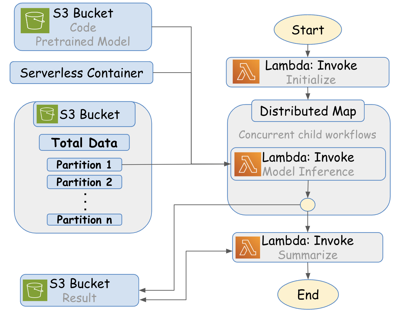
Figure 3: CAI framework overview using AWS serverless computing. It uses the AWS S3 bucket for data, code, and result storage. The state machine defines the workflow steps using AWS lambda functions and distributed maps. Parallel execution is achieved through data partitions for almost linear high-performance inference scaling.

1. Initialization: Defines the parameters and configurations of each child workflow based on the input payload. Then, it returns the parameter array with the state output. The concurrent job array size is the image data size divided by the smallest partition size. E.g. if the data and partition size is 1GB and 25MB respectively, the number of partitions is $\left\lceil 1024\div 25\right\rceil=41$.

2. Data Partitioning: The total data is split into smaller sizes so that each lambda function can work with one small partition at a time during distributed processing. We use a maximum of 25MB of data per partition (arbitrarily chosen. Section 5.7 shows results for different partition sizes). This keeps the data loading time low and allows batch data processing. This is important because too large data can potentially get out of memory (AWS Lambda has a maximum of 10GB memory).

3. Distributed Processing: This step is where concurrent job processing is done based on each input item from the initialization. It uses the following AWS components:

   • S3 Bucket: Storage for code, the pre-trained model, and data. Each child process loads the code, model, and partitioned data (assigned by the initialization state). We use the Python Boto3 library to interact and interface with our AWS S3 Bucket.

   • Serverless Container: The container is a custom AWS Lambda runtime created that includes all required software dependencies. The AWS Lambda function performing model inference is executed inside this runtime. Within this container, we also use the FMI AllReduce collective operation to capture the summation of average running time within the executing pairs of AWS Lambda serverless containers. This algorithm is highly optimized and uses a recursive doubling algorithm implemented by the library. Collectives allows for processing time delineation compared to the overall execution time reported by AWS Lambda. Additionally, with collectives, we can analyze the impact of overhead on the overall execution of our Lambda function outside the running Python code.

   • Distributed Map: The distributed map state iteratively executes its child jobs based on the input array. We can control how many jobs run concurrently. Each Lambda job has a maximum of 10GB of RAM available (AWS limitation). The model inference is done in this step independently for each partition and runs on CPU.

4. Summarize Results: The results from each job are summarized by this lambda function for final evaluation.

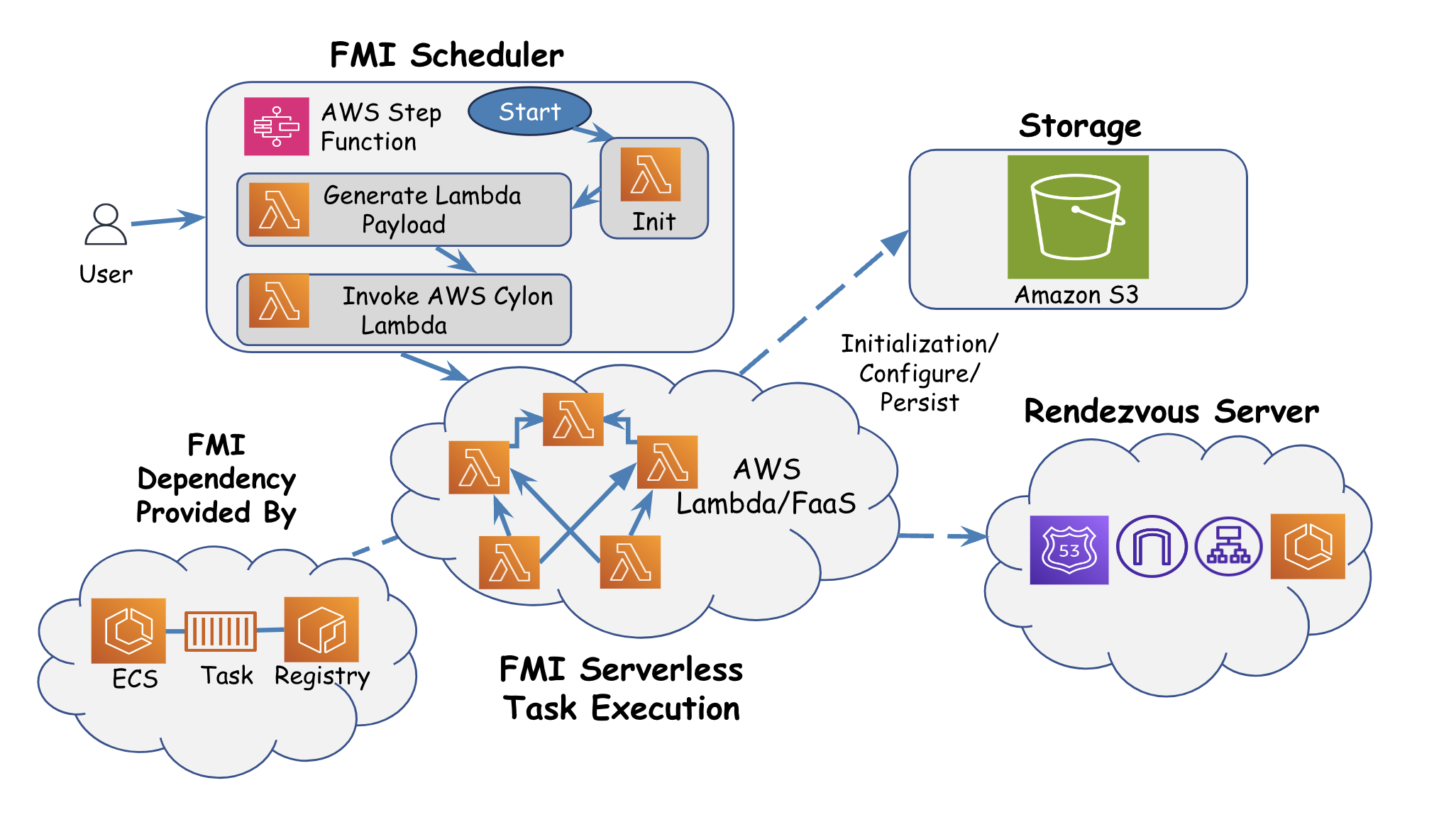
Figure 4: CAI: The Architecture of Serverless Cloud with FMI for Cosmic AI Inference.

As part of this work, we introduce and include a novel integration with FMI, FaaS Message Interface Böhringer (2022) for communication over Amazon AWS Lambda and collective operations, as illustrated in 4. This is not supported by default in AWS but offers performance benefits related to message passing between the Lambda functions. FMI supports the following collective operations: 1) send/receive, 2) broadcast, 3) gather, 4) scatter, 5) reduce, 6) all reduce, and 7) scan. Additional operations and languages can be easily added based on the abstract design of the library. FMI uses a rendezvous server during the initialization phase to exchange IP addresses and establish point-to-point connections between a pair of AWS Lambda functions. Functions can pass useful messages or perform collective operations during the later stages (e.g., model inference) once direct communication is established.

5 Experiments

We intend to showcase how CAI is a novel approach for computing redshift prediction compared to other devices. This section thoroughly outlines the dataset used in our experiment, the metrics we use to assess each device, the experimental setup, and the analysis of our results.

5.1 Dataset

The dataset used in this study is prepared following Fathkouhi and Fox (2024) and originates from Pasquet et al. (2019). It has 659,857 galaxy images derived from SDSS DR8 Aihara et al. (2011). Each image has dimensions of 64$\times$64$\times$5 and is annotated with 64 physical properties, including class, metallicity, and age, along with unique IDs for cross-referencing with other SDSS physical property tables. These images were captured using a 2.5-meter dedicated telescope at Apache Point Observatory in New Mexico and were already background-subtracted and photometrically calibrated. Pasquet et al. (2019) further processed the images by resampling them onto a common grid of overlapping frames and applying the Lánczos-3 resampling kernel Duchon (1979) to enhance image quality and reduce artifacts. The images are center-cropped to a final size of 32$\times$32$\times$5, and the magnitude values for each band, along with the redshift, are obtained using the Astroquery library Ginsburg et al. (2019). The resulting dataset, consisting of images and magnitudes as inputs and redshift as the target, is then prepared for model training.

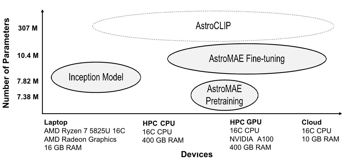
Figure 5: The parameter counts for recent deep learning-based methods developed for astronomy images, capable of inference across diverse computing environments—including a personal laptop, HPC CPUs, HPC GPUs, and our proposed cloud-based framework, CAI. A pre-trained AstroMAE model is used for the inference scaling experiments.

5.2 Implementation

We used Python 3.11 with PyTorch 2 as the core framework. Also, NumPy 1.2 and Pandas 2.2 for data analytics. Additionally, Timm 0.4.12 was independently installed to provide access to specific model architectures compatible with PyTorch Paszke et al. (2019). The FMI and Boto3 libraries were used on AWS for the CAI implementation.

5.3 AstroMAE model

AstroMAE provides two pretrained models: the first is pretrained using 80% of the data, as discussed earlier, and the second, which is employed in this study, is pretrained using the entire dataset. Both pretraining and fine-tuning are conducted on four A100 GPUs. Pretraining takes approximately three days while fine-tuning on the full dataset requires around 10 hours.

5.4 Evaluation Metrics

To determine the scalability of performing redshift inference on each device, we evaluate using the metrics outlined and defined in Table 2.

Table 2: Evaluation Metrics

Evaluation Metric	Description
Memory Capacity	Maximum Dataset Size that can complete the redshift inference (GB)
Inference Time	Total time to complete redshift inference in seconds (s)
Throughput	Bits of data transmitted per second (bps)

These metrics effectively measure scalability. Processors that can complete inference on the full dataset are strongly preferred to those that cannot due to their memory limitations. When working with large astronomy datasets, this is more crucial. Faster model inference allows researchers to conduct more analyses. Lastly, a higher throughput means more data can be processed in less time. These metrics are interdependent, and an ideal scalable framework can complete the inference on the full dataset and maximize inference throughput while minimizing time. We measure inference time using the PyTorch Profiler.

For CAI, since it is running parallel jobs, we calculate the inference time as the time needed to finish the Distributed Model Inference state (Figure 3) from the AWS step machine. The throughput is also calculated similarly, based on total bits calculated by all jobs divided by the total time to finish this state.

5.5 Experiment Setup

We compare the following processors: a personal laptop, HPC CPU, HPC GPU, and our proposed CAI. Figure 5 shows their specifications and Table 3 lists the maximum dataset size they can handle. A batch size of 512 is used throughout the experiment. Each experiment combination is repeated three times and the average metrics are reported.

Table 3: Processors’ maximum dataset size.

Processor	Maximum Dataset Size (GB)	Number of Images
Personal Laptop	8	418,323
HPC GPU	12.6 (Full dataset)	659,857
HPC CPU	12.6 (Full dataset)	659,857
CAI	12.6 (Full dataset)	659,857

First, we investigate how varying dataset sizes affect inference time, benchmarking the scalability of each device. The complete dataset is partitioned into incremental sizes: 1 GB, 2 GB, 4 GB, 6 GB, 8 GB, 10 GB, and 12.6 GB (the full dataset). This allows us to evaluate the total inference time on different devices and identify the maximum dataset size each device can handle. Second, we examine the impact of batch size on throughput (bps) across different devices. Batch sizes of 32, 64, 128, 256, and 512 are tested using a fixed dataset size of 1 GB. Finally, we evaluate the choice of partition size for CAI, using 25MB, 50MB, 75MB, and 100MB. This shows how different partition size choices could impact the inference time and throughput.

5.6 Performance Results and Analysis

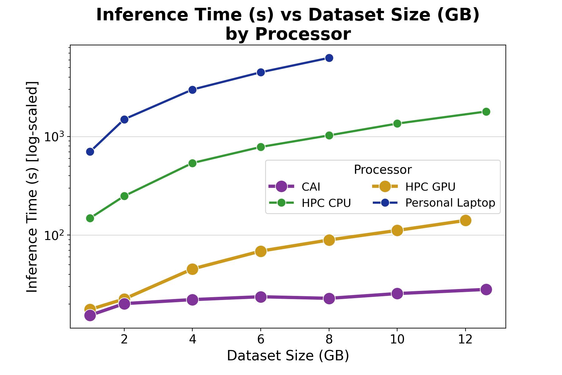
Figure 6: Inference time vs dataset size by processor (batch size 512). Each combination is run three times and the average is reported. CAI performs better than an HPC GPU with its consistent scaling with increasing data size.

Figure 6 shows that the inference time increases with data size. The personal laptop could not perform inference on the larger dataset sizes and is much slower due to memory limitations. The HPC with GPU is way faster than with CPU and personal laptop. However, CAI maintains a considerably stable inference time and performs best, due to its parallel executions, which is more evident with larger data sizes.

Model inference on the total data takes 1793 s, 140.8 s, and 28 s on the HPC CPU, HPC GPU, and CAI, respectively. The personal laptop could run to a maximum of 8GB and took 6283 s on average. This showcases personal devices are limited by memory and not feasible for the long run-times with astronomy data. Our proposed CAI is an attractive approach due to the faster inference speed despite running on CPU only.

Figure 7 shows the throughput of the devices for 1GB data size. 1GB was chosen due to the limitation of the personal laptop taking significant time with small batch size and larger data. Both the HPC GPU and CAI have significantly higher throughputs. CAI has the highest throughput (bps) for batch sizes 32, 64, and 128 (0.25B bps, 0.34B bps, and 0.42B bps respectively). The HPC GPU has the highest throughput (bps) for batch sizes 256 and 512 (0.42B bps and 0.61B bps). After CAI and the HPC GPU, the HPC CPU tends to have the next highest throughput, and then lastly, the personal laptop.

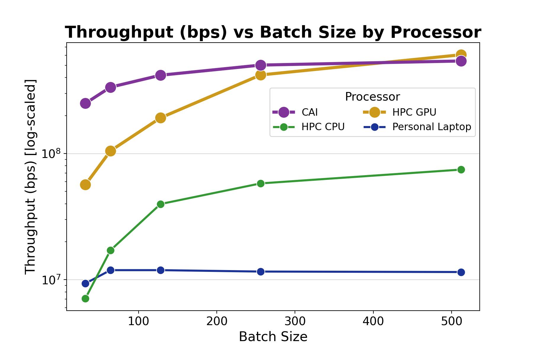
Figure 7: Average throughput (bps) vs batch size by single node device to serverless computing using the 1GB dataset on a log scale. Three executions were completed for each batch size and processor combination, and the average throughput is displayed.

The trend of throughput (bps) by the processor is that throughput (bps) increases as batch size increases, and the throughput increase rate declines with increasing batch sizes. This is because there is an overhead computation cost at the beginning of iterating through each batch. The smaller batch sizes have more batches to iterate through, so although we might expect data to be processed quicker with smaller batch sizes, the increased frequency of the overhead computational cost can add up and lower the throughput. In fact, in Figure 7, CAI appears to plateau at the batch size of 256, and the personal laptop appears to plateau at the batch size of 64.

5.7 Serverless Computing for Scalable Cosmic AI

Figure 8 shows the CAI average model inference time in seconds for different data sizes. This complements Figure 6 but shows the CAI performance in more detail. The inference time here is the runtime of the Model Inference State (Figure 3), which completes only when all concurrent Lambda functions are done. This ensures we get the correct performance in practice. The individual Lambda jobs finish much faster, but that doesn’t truly reflect the throughput.

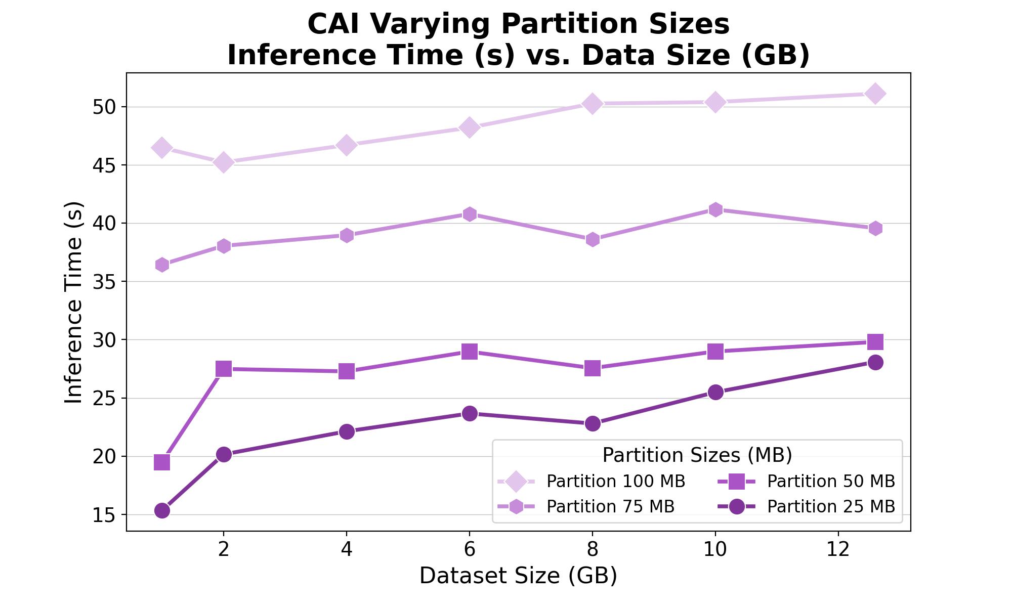
Figure 8: CAI average model inference time for different data sizes. The average time stays almost linear despite scaling up the data size due to concurrent jobs.

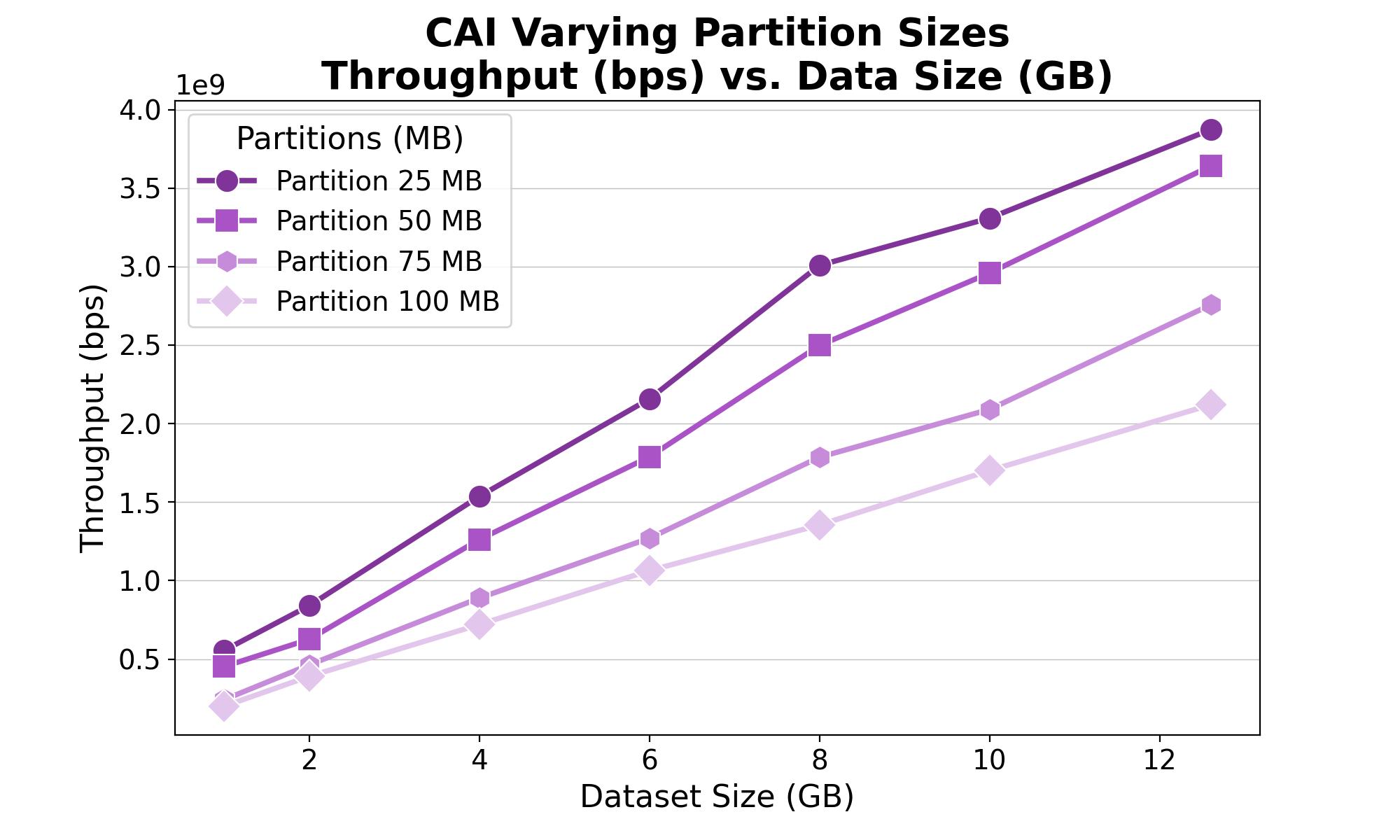
Figure 9: CAI Average Throughput for Different Data Sizes. These results are over concurrent jobs and use batch size 512) for different partition sizes.

Despite increasing the dataset size, the inference time in CAI is almost constant. For example, for the 100 MB partition, the average inference time for the 1 GB dataset is 23.02 s and only increases by 1.56 s to 24.58 s for the full 12.6 GB dataset. Furthermore, for the 25 MB partition, the average inference time for the 1 GB dataset is 6.56 s and subtly decreases by 0.73 s to 5.83 s for the full 12.6 GB dataset. This is due to the parallel processing of the large data into smaller partitions. Since each child workflow is running model inference on a small partition of data independently, the overall run time depends mostly on the execution time for that partition.

Figure 9 shows the throughput for those different partition sizes across data sizes. For each dataset size, the 25 MB partition has the highest throughput, then the 50 MB partition, then the 75 MB partition, and lastly, the 100 MB partition. At the full dataset size of 12.6 GB, the 25 MB partition has an average throughput of 18.04B bps, the 50 MB partition has an average throughput of 9.70B bps, the 75 MB partition has an average throughput of 6.66B bps, and the 100 MB partition has an average throughput of 5.12B bps. With a smaller partition, we can use more concurrent jobs, increasing the throughput.

Runtime Cost analysis: AWS Lambda costs are based on requests and the duration time related to the execution of the Lambda function. For CAI, we use three AWS Lambda functions: 1) data-parallel-init-fmi, 2) cosmic-executor, and 3) resultSummary. The material cost is the number of executions of the cosmic executor. The costs for 1) and 2) are marginal based on the fact that these are only single executions for a given job (i.e., 25GM, 50GB, 75GM, or 100GB partition(s)), and each of these lambda functions is provisioned very conservatively with 128MB memory and 512MB ephemeral storage. AWS published guidance indicates Lambda costs for the CAI use case to be based on architecture (x86 or ARM), memory, ephemeral storage, and data transfer for CAI. We have provisioned our cosmic-executor AWS Lambda function as follows:

Memory	Ephemeral	Timeout	Snapshot
10240MB	10240MB	15min0sec	None

Table 4: Data Parallel AWS Lambda configuration

The cost of invoking the CAI cosmic-executor AWS Lambda function is $0.00001667 per GB-second of computation time. It should also be mentioned that we have small S3 costs related to storage (our S3 Bucket is around 50GB) and data transfer. For the experiments conducted in the aggregate, this amounts to $0.023 per GB, and data transfer costs $0.005 per 1,000 requests. This cost is non-material, similar to costs related to executing the data-parallel-init-fmi and resultSummary AWS Lambda function. Figure 3 shows that our framework calls the Lambda function during initialization, parallel processing, and summarization. Table 5 summarizes some example cases to estimate the computation cost for our task. The number of requests is how often the Lambda function was called, which is the number of concurrent jobs (data divided by partition size).

Partition	Requests	Lambda Duration	Memory	Cost ($)
25MB	517	5.70 s	2.8GB	0.16
50MB	259	10.8 s	4.0GB	0.20
75MB	173	15.7 s	5.9GB	0.30
100MB	130	21.0 s	7.0GB	0.38

Table 5: An estimation of AWS computation cost for inference on the total dataset. Cost in US cents is $requests\times duration(s)\times memory(GB)$.

All this amounts to under five US dollars to execute the experiments. As mentioned, CAI uses the FMI library for summation and the all-reduce collective to generate metrics related to the average time required to execute the Lambda function pairs. Collective operations are used as a portable interface for parallel programming. Replacing send/receive operations with collectives increases performance and facilitates debugging and maintenance. Collectives also lead to a ”…”division of labor: the programmer thinks in terms of these primitives and the library is responsible for implementing them efficiently.”Peter Sanders (2009). For example, we determined the average summation time to be measured across twelve AWS Lambda functions for a 1 GB partition processing inference to be 44.012 seconds without resorting to manual calculation or another process to calculate this result. This accurately measures the processing time across AWS Lambda functions and allows researchers a clear view of execution time as a function of cost. One novelty aspect of CAI is related to the costs of executing astronomy inference compared to similar costs on HPC clusters or other ”rack and stack infrastructure.” Coupling this with the integration of FMI allows researchers to utilize a configured lambda function’s processing capability fully. With FMI, we can configure a fleet of AWS Lambda functions and bypass a subset of the costs related to invocation by using communication between AWS Lambda functions in the form of Nat Traversal or point-to-point communication.

6 Conclusion and Future Work

This paper presents a novel cloud-based framework, CAI, designed to enhance the inference scalability of foundation models trained on astronomical images. Our study highlights the essential role of cloud services in overcoming the computational and storage challenges inherent in modern astronomical research. We have leveraged serverless computing to enhance the scalability of foundation models via partitions and data parallel optimizations.

To showcase the attractive capabilities of CAI, we used a recent foundation model, fine-tuned for redshift prediction, in our experiments. Comprehensive evaluations across varying dataset sizes and computing devices demonstrate CAI’s robustness in scaling almost linearly on the inference and high throughput for large-scale astronomical image datasets. Note that this framework can be applied to additional critical astronomy inference tasks, such as morphology classification and star formation history. Future work will also involve testing other foundation models developed for astronomical images and spectra. Moreover, we plan to integrate the FMI communication interface into the open-source Cylon Perera et al. (2024) library. This will build upon the high-performance communication libraries currently supported (e.g., MPI, UCC/UCX, Gloo).

7 Acknowledgement

This work is partly supported by NSF grant CCF-1918626 Expeditions: Collaborative Research: Global Pervasive Computational Epidemiology, and NSF Grant 2200409 for CyberTraining:CIC: CyberTraining for Students and Technologies from Generation Z.

References

- Aihara et al. (2011) Aihara H, Prieto C, An D et al. (2011) The eighth data release of the sloan digital sky survey: first data from sdss-iii. The Astrophysical Journal Supplement Series 193(2): 29.
- AWS (2024) AWS (2024) Serverless. https://aws.amazon.com/serverless .
- Böhringer (2022) Böhringer R (2022) Fmi: The faas message interface. In: Master’s thesis, ETH Zurich.
- Chen et al. (2020) Chen T, Kornblith S, Norouzi M and Hinton G (2020) A simple framework for contrastive learning of visual representations. In: III HD and Singh A (eds.) Proceedings of the 37th International Conference on Machine Learning, Proceedings of Machine Learning Research, volume 119. PMLR, pp. 1597–1607. URL https://proceedings.mlr.press/v119/chen20j.html.
- De Prado et al. (2014) De Prado R, García-Galán S, Expósito J, López L and Reche R (2014) Processing astronomical image mosaic workflows with an expert broker in cloud computing. Image Processing & Communications 19(4): 5.
- Devlin (2018) Devlin J (2018) Bert: Pre-training of deep bidirectional transformers for language understanding. arXiv preprint arXiv:1810.04805 .
- Dosovitskiy (2020) Dosovitskiy A (2020) An image is worth 16x16 words: Transformers for image recognition at scale. arXiv preprint arXiv:2010.11929 .
- Duchon (1979) Duchon C (1979) Lanczos filtering in one and two dimensions. Journal of Applied Meteorology and Climatology 18(8): 1016–1022.
- Faaique (2024) Faaique M (2024) Overview of big data analytics in modern astronomy. International Journal of Mathematics, Statistics, and Computer Science 2: 96–113.
- Fan et al. (2019) Fan X, McGreer I, Patej A, Alvarez A, Choi Y, Jannuzi B and Zaritsky D (2019) Overview of the desi legacy imaging surveys.
- Fathkouhi and Fox (2024) Fathkouhi A and Fox G (2024) Astromae: Redshift prediction using a masked autoencoder with a novel fine-tuning architecture. In: 2024 IEEE 20th International Conference on e-Science (e-Science). IEEE, pp. 1–10.
- Gill and Buyya (2020) Gill SS and Buyya R (2020) Failure management for reliable cloud computing: A taxonomy, model, and future directions. Computing in Science & Engineering 22(3): 52–63. 10.1109/MCSE.2018.2873866.
- Ginsburg et al. (2019) Ginsburg A, Sipőcz B, Brasseur C et al. (2019) Astroquery: an astronomical web-querying package in python. The Astronomical Journal 157(3): 98.
- Gunn et al. (1998) Gunn J, Carr M, Rockosi C, Sekiguchi M, Berry K, Elms B and Brinkman J (1998) The sloan digital sky survey photometric camera. The Astronomical Journal 116(6): 3040.
- Hayat et al. (2021) Hayat M, Stein G, Harrington P, Lukić Z and Mustafa M (2021) Self-supervised representation learning for astronomical images. The Astrophysical Journal Letters 911(2): L33.
- Henghes et al. (2022) Henghes B, Thiyagalingam J, Pettitt C, Hey T and Lahav O (2022) Deep learning methods for obtaining photometric redshift estimations from images. Monthly Notices of the Royal Astronomical Society 512(2): 1696–1709.
- Hubble (1929) Hubble E (1929) A relation between distance and radial velocity among extra-galactic nebulae. Proceedings of the National Academy of Sciences 15(3): 168–173.
- Jones et al. (2024) Jones E, Do T, Li YQ, Alfaro K, Singal J and Boscoe B (2024) Redshift prediction with images for cosmology using a bayesian convolutional neural network with conformal predictions. The Astrophysical Journal 974(2): 159.
- Khlamov et al. (2022) Khlamov S, Savanevych V, Briukhovetskyi O, Trunova T and Tabakova I (2022) Colitec virtual observatory platform for the cloud computing analysis of light curves for the variable stars. In: 2022 IEEE 9th International Conference on Problems of Infocommunications, Science and Technology (PIC S&T). IEEE, pp. 1–4.
- Kim and Hahm (2011) Kim H and Hahm J (2011) Light-weight cloud job management system for data intensive science. In: 2011 Fourth IEEE International Conference on Utility and Cloud Computing. pp. 377–381. 10.1109/UCC.2011.63.
- Lanusse et al. (2023) Lanusse F, Parker L, Golkar S, Bietti A, Cranmer M, Eickenberg M and Ho S (2023) Astroclip: cross-modal pre-training for astronomical foundation models. In: NeurIPS 2023 AI for Science Workshop.
- Li et al. (2022) Li Y, Lin Y, Wang Y, Ye K and Xu C (2022) Serverless computing: state-of-the-art, challenges and opportunities. IEEE Transactions on Services Computing 16(2): 1522–1539.
- Murrugarra-Llerena and Hirata (2017) Murrugarra-Llerena J and Hirata N (2017) Galaxy image classification. In: E-Proceedings.
- Neely (2021) Neely B (2021) Cloudy with a chance of peptides: accessibility, scalability, and reproducibility with cloud-hosted environments. Journal of Proteome Research 20(4): 2076–2082.
- Parra-Royón et al. (2024) Parra-Royón M, Rodríguez-Gallardo Á, Sánchez-Expósito S et al. (2024) Bringing computation to the data: A moea-driven approach for optimising data processing in the context of the ska and srcnet. In: 2024 IEEE International Conference on Evolving and Adaptive Intelligent Systems (EAIS). IEEE, pp. 1–8.
- Pasquet et al. (2019) Pasquet J, Bertin E, Treyer M et al. (2019) Photometric redshifts from sdss images using a convolutional neural network. Astronomy & Astrophysics 621: A26.
- Paszke et al. (2019) Paszke A, Gross S, Massa F, Lerer A, Bradbury J, Chanan G, Killeen T, Lin Z, Gimelshein N, Antiga L et al. (2019) Pytorch: An imperative style, high-performance deep learning library. Advances in neural information processing systems 32.
- Perera et al. (2024) Perera N, Sarker AK, Shan K, Fetea A, Kamburugamuve S, Kanewala TA, Widanage C, Staylor M, Zhong T, Abeykoon V et al. (2024) Supercharging distributed computing environments for high-performance data engineering. Frontiers in High Performance Computing 2: 1384619.
- Peter Sanders (2009) Peter Sanders aJLT JochenS Peck (2009) Two-treealgorithms for full bandwidth broadcast, reduction and scan. Parallel Comput : 581–594.
- Sen et al. (2022) Sen S, Agarwal S, Chakraborty P et al. (2022) Astronomical big data processing using machine learning: A comprehensive review. Experimental Astronomy 53: 1–43. 10.1007/s10686-021-09827-4.
- Wang et al. (2022) Wang D, Zhang Q, Xu Y et al. (2022) Advancing plain vision transformer toward remote sensing foundation model. IEEE Transactions on Geoscience and Remote Sensing 61: 1–15.
- Willett et al. (2013) Willett K, Lintott C, Bamford S, Masters K, Simmons B, Casteels K and Thomas D (2013) Galaxy zoo 2: detailed morphological classifications for 304,122 galaxies from the sloan digital sky survey. Monthly Notices of the Royal Astronomical Society 435(4): 2835–2860.
- Zhang et al. (2020) Zhang Z, Barbary K, Nothaft FA, Sparks ER, Zahn O, Franklin MJ, Patterson DA and Perlmutter S (2020) Kira: Processing astronomy imagery using big data technology. IEEE Transactions on Big Data 6(2): 369–381. 10.1109/TBDATA.2016.2599926.