A partition cover approach to tokenization

Abstract

Tokenization is the process of encoding strings into tokens from a fixed vocabulary of size $k$ and is widely utilized in Natural Language Processing applications. The leading tokenization algorithm today is Byte Pair Encoding (BPE), which formulates the tokenization problem as a compression problem and tackles it by performing sequences of merges. In this work, we formulate tokenization as an optimization objective, show that it is NP-hard via a simple reduction from vertex cover, and propose a polynomial-time greedy algorithm GreedTok. Our formulation naturally relaxes to the well-studied weighted maximum coverage problem which has a simple $(1-1/e)$-approximation algorithm GreedWMC. Through empirical evaluations on real-world corpora, we show that GreedTok outperforms BPE, while achieving a comparable objective score as GreedWMC (which could have achieved a higher score due to relaxation).

1 Introduction

Tokenization is the process of encoding strings into tokens from a fixed vocabulary of size $k$ and is widely utilized in Natural Language Processing (NLP) applications. With the growing popularity of Large Language Models (LLMs) today, there is significant interest in improving our understanding of tokenization as tokenization is integral to the architecture of these LLMs. It is not unthinkable that even a minor increase in tokenization performance can result in reasonable accumulated savings in compute resources. For instance, LLMs such as LLaMA [TLI⁺23] and Mistral [JSM⁺23] use fixed-length context windows that may benefit from tokenizers with better compression utility enabling the fitting of more information within its context window. There are also prompt-based [WWS⁺22, YYZ⁺23] and finetuning [FTL⁺23] strategies to improve LLM performance by increasing the number of tokens processed.

A common way to formalize the tokenization problem is to frame it as a compression problem where one tries to minimize the ratio of tokens produced from tokenizing the input data. The leading tokenization algorithm today is Byte Pair Encoding (BPE) [Gag94, SHB16], chosen by most LLMs [KHM⁺23], which formulates the tokenization problem as a compression problem and tackles it by performing a sequence of pairwise merges. Due to its popularity, there have been a multitude of recent works analyzing the theoretical properties of BPE [ZMG⁺23, KV24, WBP24].

Contributions.

In this work, we deviate from the usual compression ratio formulation of tokenization and merge-based algorithms.

1. We formulate an optimization objective formulation of the tokenization problem which is more general than the merge-based ones in prior works [ZMG⁺23, KV24]. These prior formulations are based on merging tokens in a bottom-up fashion where they restrict any solution to construct tokens from the existing set of tokens in pairwise merges. However, the idea of tokenization is simply to efficiently represent a corpus with a judiciously selected set of tokens, whose construction is independent of such merge patterns. As we will see, our formulation does not have such merging requirements and subsumes these prior formulations in the following sense: a solution to these prior formulations is valid in our formulation while a solution to our general formulation need not be based on bottom-up parwise merges.

2. We provide a simple and intuitive proof that tokenization is NP-hard in our optimization objective formulation via a reduction from vertex cover [Kar72]. While there has a been a recent concurrent work [WBP24] that also showed that the tokenization problem is NP-hard, our proof is arguably simpler due to our formulation.

3. We propose a polynomial-time greedy algorithm GreedTok that does not rely on a sequence of pairwise token merges. Instead, GreedTok only requires an ordering of the chosen tokens, facilitating the use of custom token sets in solving the tokenization problem; see Section 4.3 and the discussion in Section 6. We evaluated GreedTok against BPE on four real-world corpora, at different compression utility (mean number of tokens per word) targets. Our empirical evaluations showed that GreedTok outperforms BPE in terms of compression utility, with an average of 3% and up to 5% fewer tokens per word when compared on the same vocabulary size $k$. To reach similar compression utility, our experiments show that GreedTok requires an average 13% fewer number of tokens than BPE. Our implementation and experiments can be found at https://github.com/PreferredAI/pcatt.

4. While we do not have any formal approximation guarantees for GreedTok at this point in time, since our formulation naturally relaxes to the well-studied weighted maximum coverage problem [Kar72, CK08] which has a simple $(1-1/e)$-approximation algorithm GreedWMC [Hoc96], we empirically show that GreedTok and GreedWMC achieve a similar objective function value for large $k$, which holds for practical scenarios, despite the latter being a relaxed problem.

Related work.

Recently, there are a flurry of works that seek to analyze tokenization. Zouhar et al. [ZMG⁺23] first attempted the formalization of BPE with their formulation (bottom-up tokenization problem) restricting the sequential inclusion of new tokens to be built from merges between two tokens in the existing vocubulary. Kozma and Voderholzer [KV24] is another concurrent work proving bottom-up tokenization problem, and its more general variant, is APX-complete using linear reduction [PY88] from maximum cut [Kar72] in cubic graphs. They also showed that BPE approximates a worst-case factor of between 0.333 and 0.625 for their general variant. Whittington, Bachmann, and Pimentel [WBP24] is a concurrent work that proved that the general tokenization problem (direct tokenization problem in their work) and bottom-up tokenization problem are NP-complete from the reduction of the maximum 2-satisfiability problem. The smallest grammar problem [CLL⁺05] is a kind of compression problem different from the tokenization problem. Their differences, mainly tokenization compresses using a fixed $k$ token vocabulary size, are elegantly explained in [WBP24]. Aside from theoretical analysis, there are also empirical-based investigations, such as [LBM23] and [SFWN23] that examine the practical downstream impact of tokenizer selection on NLP problems. Compared to the previous and concurrent works, our NP-hardness proof is arguably simpler due to our formulation. We also provide a new tokenization algorithm that is empirically competitive in NLP scenarios.

Outline of paper.

After giving our general optimization formulation for tokenization in Section 2, we prove that it is NP-hard in Section 3. GreedTok is designed in Section 4 and Section 5 contains our empirical evaluation against real world corpora. Finally, we conclude with some discussions in Section 6.

Notation.

We use standard set notations such as $|\mathbf{A}|$ to represent the size of set $\mathbf{A}$, and standard asymptotic notations such as $O(\cdot)$. Numbers are represented with small letters, strings/words with capital letters, and sets with bold letters. Unordered sets are denoted by $\{\cdot\}$ and ordered tuples are denoted by $(\cdot)$. We describe words in plaintext, e.g., hello, or as a tuple of singletons, e.g., (h,e,l,l,o).

2 A general optimization formulation for the tokenization problem

Let us fix an alphabet $\mathbf{\Sigma}$ of interest. A corpus $\mathcal{C}=(\mathbf{W},\textsc{count})$ is a collection of words $\mathbf{W}\subseteq\mathbf{\Sigma}^{+}$ and count function $\textsc{count}:\mathbf{W}\to\mathbb{N}$. Meanwhile, for any word $W\in\mathbf{\Sigma}^{+}$ and a given set of tokens $\mathbf{S}\subseteq\mathbf{\Sigma}^{+}$, $\textsc{partition}(W,\mathbf{S})$ is the minimum number of tokens from $\mathbf{S}$ that can sequentially concatenate to form $W$. For example, the word $W=\text{abc}$ can be formed by concatenating tokens ab and c, but not with tokens ac and b, although the union of symbols in both cases generates the symbols of $W$. The metric of using small number of total tokens to represent a corpus is also sometimes referred to as the compression utility.

Problem 1 (The tokenization search problem Tok).

Fix an alphabet set $\mathbf{\Sigma}$ and define $\mathbf{B}=\{(W):W\in\mathbf{\Sigma}\}$ as the base set of singleton tokens. Given positive integers $k$, a corpus $\mathcal{C}=(\mathbf{W},\textsc{count})$, and a set of candidate tokens $\mathbf{T}\subseteq\mathbf{\Sigma}^{+}$, the tokenization problem is to find a subset $\mathbf{S}\subseteq\mathbf{T}$ of tokens such that $|\mathbf{S}|\leq k$ and $\sum_{W\in\mathbf{W}}\textsc{partition}(W,\mathbf{S}\cup\mathbf{B})\cdot\textsc{count}(W)$ is minimized.

When proving that a problem is NP-hard, one typically transforms it into its decision variant because NP-hardness is defined in terms of decision problems. Once the decision variant is proven to be NP-hard, the corresponding search problem is also said to be NP-hard because solving the search variant implicitly solves the decision variant since one can search over the problem parameters (in our case, the value $\ell$).

Problem 2 (The tokenization decision problem).

Fix an alphabet set $\mathbf{\Sigma}$ and define $\mathbf{B}=\{(W):W\in\mathbf{\Sigma}\}$ as the base set of singleton tokens. Given positive integers $k,\ell\in\mathbb{N}_{>0}$, a corpus $\mathcal{C}=(\mathbf{W},\textsc{count})$, and a set of candidate tokens $\mathbf{T}\subseteq\mathbf{\Sigma}^{+}$, the tokenization problem is to decide whether there is a subset $\mathbf{S}\subseteq\mathbf{T}$ of tokens such that $|\mathbf{S}|\leq k$ and $\sum_{W\in\mathbf{W}}\textsc{partition}(W,\mathbf{S}\cup\mathbf{B})\cdot\textsc{count}(W)\leq\ell$.

There is a subtle difference between our formulation and the prior formulations of the tokenization problem, such as those in [ZMG⁺23, KV24]. Instead of viewing the problem as a form of string compression, our formulation boils the tokenization problem down to a simple question: Are two adjacent singletons within a string represented by the same token? This is because the essence of tokenization only requires that each singleton of every word is represented by exactly one token from the final token set. This viewpoint frees us from the perspective of designing merge sequences which we view as an artefact of analyses based off algorithms that rely on merge sequences for tokenization, such as BPE. We further discuss our formulation in Section 4.2.

3 Tokenization is NP-hard

In this section, we will prove that the tokenization decision problem (Problem 2) is NP-hard by reducing the vertex cover problem, which is known to be NP-hard [Kar72], to it. Given a graph $\mathcal{G}=(\mathbf{V},\mathbf{E})$, where $\mathbf{V}$ is the set of vertices and $\mathbf{E}$ is the set of edges, a vertex cover is a subset $\mathbf{S}\subseteq\mathbf{V}$ of vertices such that $|\mathbf{S}\cap\{U,V\}|\geq 1$ for every edge $\{U,V\}\in\mathbf{E}$. The decision variant of the vertex cover problem is then to decide whether a given graph $\mathcal{G}$ has a vertex cover of size at most a given integer $k$.

Theorem 1.

The tokenization problem is NP-hard.

Proof.

We will prove this by reducing the vertex cover problem, which is known to be NP-hard [Kar72], to the tokenization problem. Given an arbitrary vertex cover problem instance, we show how to construct a corresponding tokenization instance. Then, we argue that the derived tokenization problem instance is a YES instance if and only if the original vertex cover problem instance is a YES instance. In this proof, for clarity, we will write words $W\in\mathbf{W}$ as a tuple of singletons instead of usual plaintext, e.g. (h,e,l,l,o) instead of hello.

Construction.

Consider an arbitrary vertex cover problem given by the graph $\mathcal{G}=(\mathbf{V},\mathbf{E})$ over $n$ vertices $\mathbf{V}=\{V_{1},\ldots,V_{n}\}$ and a positive integer $k\in\mathbb{N}_{\geq 0}$. To construct an instance of the tokenization problem, we first define the alphabet as follows: $\mathbf{\Sigma}=\{V_{1},\ldots,V_{n},@\}$ where $@$ is an additional symbol which we will use later. So, we have $\mathbf{B}=\{(V_{1}),\ldots,(V_{n}),(@)\}$. For each edge $\{V_{i},V_{j}\}\in\mathbf{E}$ with $i<j$, we create a word $W_{i,j}=(@,V_{i},@,V_{j},@)$ and define the set of words as $\mathbf{W}=\{W_{i,j}:\{V_{i},V_{j}\}\in\mathbf{E}\}$ where each word has count 1, i.e. $\textsc{count}(W)=1$ for all $W\in\mathbf{W}$. Then, we define the set of candidate tokens $\mathbf{T}=\{(@,V_{i},@):V_{i}\in\mathbf{V}\}$. Finally, we set $\ell=3|\mathbf{W}|=3|\mathbf{E}|$ and associate the parameter $k$ in the vertex cover problem instance to the corresponding parameter $k$ in the tokenization problem instance. One can check that this derived tokenization instance can be constructed in polynomial time.

Observation.

Observe that every word $W\in\mathbf{W}$ has length 5 and each token in $\mathbf{S}$ has length 3, so $\textsc{partition}(W,\mathbf{S}\cup\mathbf{B})$ will either be 3, when there is some token in $\mathbf{S}$ that is a contiguous subword of $W$, or 5 otherwise. For instance, given the word $W_{i,j}=(@,V_{i},@,V_{j},@)$, we have $\textsc{partition}(W_{i,j},\mathbf{S}\cup\mathbf{B})=3$ if and only if at least one of $(@,V_{i},@)$ or $(@,V_{j},@)$ is chosen in $\mathbf{S}$ (both could be in $\mathbf{S}$). Furthermore, since all words have count 1, the tokenization problem becomes finding $\mathbf{S}\subseteq\mathbf{T}$ such that $|\mathbf{S}|\leq k$ and $\sum_{W\in\mathbf{W}}\textsc{partition}(W,\mathbf{S}\cup\mathbf{B})\leq\ell=3|\mathbf{W}|$.

YES instance of tokenization problem to YES instance of vertex cover.

Suppose there exists a subset $\mathbf{S}\subseteq\mathbf{T}$ of tokens such that $|\mathbf{S}|\leq k$ and $\sum_{W\in\mathbf{W}}\textsc{partition}(W,\mathbf{S}\cup\mathbf{B})\leq\ell=3|\mathbf{W}|$. Then, from the observation above, we know that this can only happen when $\textsc{partition}(W,\mathbf{S}\cup\mathbf{B})=3$ for every $W\in\mathbf{W}$. This implies that for each word $W_{i,j}$, at least one of $(@,V_{i},@)$ or $(@,V_{j},@)$ is chosen in $\mathbf{S}$. Therefore, $\mathbf{S}_{\mathcal{G}}=\{V_{i}\in\mathbf{V}:(@,V_{i},@)\in\mathbf{S}\}$ is a subset of size $|\mathbf{S}_{\mathcal{G}}|=|\mathbf{S}|\leq k$ and corresponds to a vertex cover of the original graph $\mathcal{G}$.

YES instance of vertex cover to YES instance of tokenization problem.

Suppose the original vertex cover instance for graph $\mathcal{G}=(\mathbf{V},\mathbf{E})$ has a vertex cover $\mathbf{S}_{\mathcal{G}}$ of size $|\mathbf{S}_{\mathcal{G}}|\leq k$. Then, let us define $\mathbf{S}=\{(@,V_{i},@)\in\mathbf{\Sigma}^{+}:V_{i}\in\mathbf{S}_{\mathcal{G}}\}$ as the set of chosen tokens of size $|\mathbf{S}|=|\mathbf{S}_{\mathcal{G}}|\leq k$. Since $\mathbf{S}_{\mathcal{G}}$ is a set cover for $\mathcal{G}$, by construction of $\mathbf{W}$, we see that $\textsc{partition}(W,\mathbf{S}\cup\mathbf{B})=3$ for all $W\in\mathbf{W}$. Therefore, $\sum_{W\in\mathbf{W}}\textsc{partition}(W,\mathbf{S}\cup\mathbf{B})=3|\mathbf{W}|$. ∎

Example 1.

Consider a vertex cover instance on a graph $\mathcal{G}=(\mathbf{V},\mathbf{E})$ with vertices $\mathbf{V}=\{V_{1},\ldots,V_{5}\}$ and edges $\mathbf{E}=\{\{V_{1},V_{2}\},\{V_{1},V_{4}\},\{V_{1},V_{5}\},\{V_{2},V_{3}\},\{V_{2},V_{4}\},\{V_{3},V_{5}\}\}$ where the subset $\mathbf{S}=\{V_{1},V_{3},V_{4}\}$ is a vertex cover of size $|\mathbf{S}|=k=3$. Fig. 1 illustrates the corresponding tokenization problem instance created according to the construction in the proof of Theorem 1.

Figure 1: An example tokenization problem instance construction according to the proof of Theorem 1. The tokens corresponding to the vertex cover $\mathbf{S}=\{V_{1},V_{3},V_{4}\}$ are underlined in $\mathbf{T}$. A possible tokenization of $\mathbf{W}$ using $\mathbf{S}\cup\mathbf{B}$ is also given with tokens in $\mathbf{S}$ being underlined, showing that each word in $\mathbf{W}$ only needs 3 tokens.

4 GreedTok: Our greedy tokenization algorithm

4.1 Challenges in designing an efficient algorithm for Problem 1

Earlier, in Section 3, we showed that the tokenization problem is NP-hard. Developing efficient algorithms for NP-hard problems typically involves strategies that trade off between exactness, runtime, and solution quality. Since we are interested in efficient and practical solutions to the tokenization problem on large instances, we look towards developing approximate solutions that run in polynomial time, i.e. we would forgo the idea of designing a fixed-parameter tractable algorithms. In the following, we discuss two common approaches to design efficient algorithms for NP-hard problems with provable approximation guarantees and explain why they do not work for our situation.

The first approach is to show that the problem at hand is submodular or supermodular, and then apply known algorithmic frameworks to design a corresponding solution. For example, submodular problems are known to admit $(1-1/e)$-approximate greedy algorithms [NWF78]. Using $2^{\mathbf{T}}$ to denote the powerset of $\mathbf{T}$, submodular and supermodular set functions are defined as follows:

Definition 2 (Submodular Set Function).

A real-valued set function $f:2^{\mathbf{T}}\to\mathbb{R}$ is submodular if $f(\mathbf{A}\cup\{C\})-f(\mathbf{A})\geq f(\mathcal{A}\cup\{C\})-f(\mathcal{A})$ for all $\mathbf{A}\subseteq\mathcal{A}\subseteq\mathbf{T}$ and $C\in\mathbf{T}\setminus\mathcal{A}$.

Definition 3 (Supermodular Set Function).

A real-valued set function $f:2^{\mathbf{T}}\to\mathbb{R}$ is supermodular if $f(\mathbf{A}\cup\{C\})-f(\mathbf{A})\leq f(\mathcal{A}\cup\{C\})-f(\mathcal{A})$ for all $\mathbf{A}\subseteq\mathcal{A}\subseteq\mathbf{T}$ and $C\in\mathbf{T}\setminus\mathcal{A}$.

Informally speaking, submodular functions represent diminishing returns while supermodular functions represent increasing returns. In the context of the tokenization problem, the set $\mathbf{T}$ represents the candidate set of all possible tokens. Unfortunately for us, Problem 1 is neither submodular nor supermodular; see Table 1.

Single word corpus $W=\text{scaredy}$ with $\textsc{count}(W)=1$
Case 1		Case 2
$\mathbf{X}=\{\text{care}\}$	$f(\mathbf{X})=f(\mathbf{X}\cup\{Z\})=4$	$\mathbf{X}=\{\text{care}\}$	$f(\mathbf{X})=4$
$\mathbf{Y}=\{\text{care, edy}\}$	$f(\mathbf{Y})=4$	$\mathbf{Y}^{\prime}=\{\text{care, scared}\}$	$f(\mathbf{Y}^{\prime})=f(\mathbf{Y}^{\prime}\cup\{Z^{\prime}\})=2$
$Z=\text{scar}$	$f(\mathbf{Y}\cup\{Z\})=2$	$Z^{\prime}=\text{dy}$	$f(\mathbf{X}\cup\{Z^{\prime}\})=3$
$0=f(\mathbf{X}\cup\{Z\})-f(\mathbf{X})>f(\mathbf{Y}\cup\{Z\})-f(\mathbf{Y})=-2$		$-1=f(\mathbf{X}\cup\{Z^{\prime}\})-f(\mathbf{X})<f(\mathbf{Y}^{\prime}\cup\{Z^{\prime}\})-f(\mathbf{Y}^{\prime})=0$

Table 1: The above table shows that the objective function of Problem 1 is neither supermodular nor submodular. Suppose we wish to tokenize the word $W=\text{scaredy}$ with candidate token set $\mathbf{T}=\{\text{care, edy, scar, scared, dy}\}$ and singletons $\{\text{s,c,a,r,e,d,y}\}$, and the function $f$ outputs the smallest possible number of final tokens used to represent $W$, i.e. the objective function of Problem 1 on a single word corpus. Observe that $\mathbf{X}\subseteq\mathbf{Y}\subseteq\mathbf{T}$, $Z\in\mathbf{T}\setminus\mathbf{Y}$, $\mathbf{X}\subseteq\mathbf{Y}^{\prime}\subseteq\mathbf{T}$, and $Z^{\prime}\in\mathbf{T}\setminus\mathbf{Y}^{\prime}$. In case 1, using $\mathbf{X}$ to tokenize $W$ results in using 4 tokens $(\text{s, care, d, y})$ and one can check that using $\mathbf{X}\cup\{Z\}$ also results in 4 tokens. On the other hand, using $\mathbf{Y}$ results in 4 tokens $(\text{s, care, d, y})$ but using $\mathbf{Y}\cup\{Z\}$ results in 2 tokens $(\text{scar, edy})$. Therefore, $f(\mathbf{X}\cup\{Z\})-f(\mathbf{X})>f(\mathbf{Y}\cup\{Z\})-f(\mathbf{Y})$ and thus $f$ is not supermodular. On the other hand, in case 2, using $\mathbf{Y}^{\prime}$ and $\mathbf{Y}^{\prime}\cup\{Z^{\prime}\}$ to tokenize $W$ results in 2 tokens $(\text{scared, y})$ while using $\mathbf{X}\cup\{Z^{\prime}\}$ results in 3 tokens $(\text{s, care, dy})$. Therefore, $f(\mathbf{X}\cup\{Z^{\prime}\})-f(\mathbf{X})<f(\mathbf{Y}^{\prime}\cup\{Z^{\prime}\})-f(\mathbf{Y}^{\prime})$ and thus $f$ is not submodular.

The second approach is to relax the original problem into one that is efficiently solvable and then prove approximation guarantees by relating between the relaxed solution to the original problem. For example, one can formulate the NP-hard vertex cover problem as an integer linear program, relax the integral constraints, solve the resulting linear program in polynomial time, and round the fractional solution back into an integral solution that corresponds to an actual vertex cover. This approach yields a 2-approximation algorithm for the vertex cover problem, e.g. see [WS11, Section 1.2]. Alas, real-world NLP problems involve large corpora which translates to problem instances with an extremely large number of variables and constraints which makes this relax-and-round paradigm practically infeasible.

4.2 An equivalent mixed integer program formulation

To design our algorithm GreedTok for the tokenization problem, we first show an equivalent formulation of Problem 1 in terms of a mixed integer program (MIP). The rationale behind this is two-fold. First, the MIP formulation offers a more straightforward and intuitive framework for defining our greedy algorithm. This clarity simplifies the process of understanding and implementing the algorithm within the given constraints. Second, the MIP formulation naturally lends itself to a relaxation to the well-established weighted maximum coverage problem (WMC), which is known to be submodular and has a corresponding greedy algorithm GreedWMC that provably achieves an $(1-1/e)$-approximation; see [Hoc96, Section 3.9]. While we are unable to formally prove guarantees for GreedTok, the relaxation to WMC allows us to empirically evaluate the performance of GreedTok on tokenization problem instances via a comparison to GreedWMC.

To begin, let us define $\textsc{cover}(W,\mathbf{S})$ as the maximum number of adjacent singletons in $W$ that can be concatenated to form tokens in $\mathbf{S}$ without using any singleton more than once. Now, recalling the definition of $\textsc{partition}(W,\mathbf{S}\cup\mathbf{B})$ from Problem 1, we see that $|W|+1=\textsc{partition}(W,\mathbf{S}\cup\mathbf{B})+\textsc{cover}(W,\mathbf{S})$ for any word $W$. For example, $\textsc{cover}(W=\text{scaredy},\mathbf{S}=\{\text{care, edy}\})=4$ since we can concatenate adjacent singletons $(\text{c,a,r,e})$ into $\text{care}\in\mathbf{S}$. Note that $\textsc{cover}(W=\text{scaredy},\mathbf{S}=\{\text{care, edy}\})\neq 4+3=7$ because we cannot use the singleton ‘e’ twice. Meanwhile, $\textsc{partition}(W=\text{scaredy},\mathbf{S}\cup\mathbf{B}=\{\text{care, edy}\}\cup\{\text{s,c,a,r,e,d,y}\})=4$ via s␣care␣d␣y, where ␣ represents a split between the tokens. Thus, we can rewrite the minimization objective using partition in Problem 1 in terms of a maximization objective using cover:

$$\;\min\sum_{W\in\mathbf{W}}\textsc{count}(W)\cdot\textsc{partition}(W,\mathbf{S}\cup\mathbf{B})$$

$$= \;\min\sum_{W\in\mathbf{W}}\textsc{count}(W)\cdot(|W|+1-\textsc{cover}(W,\mathbf{S})) |W|+1=\textsc{partition}(W,\mathbf{S}\cup\mathbf{B})+\textsc{cover}(W,\mathbf{S})$$ (Since )

$$= \;\max\sum_{W\in\mathbf{W}}\textsc{count}(W)\cdot(\textsc{cover}(W,\mathbf{S})-|W|-1)$$

$$= \;\max\sum_{W\in\mathbf{W}}\textsc{count}(W)\cdot\textsc{cover}(W,\mathbf{S}) \sum_{W\in\mathbf{W}}\textsc{count}(W)\cdot(|W|+1) \mathcal{C}=(\mathbf{W},\textsc{count})$$ (Since is a constant with respect to the corpus )

Henceforth, we use Tok to refer to both minimization and maximization versions of the tokenization problem.

Now, recall that $\mathbf{W}$ represents the set of words in the corpus with each word $W=(W_{1},\ldots,W_{|W|})\in\mathbf{W}$ having length $|W|$ and $\textsc{count}(W)\geq 1$. Although our general formulation allows for any possible set of candidate tokens $\mathbf{T}$, we need to consider all possible substrings of length $\geq 2$ in order to find an optimal solution for the given corpus. There are at most $|\mathbf{T}|\leq\sum_{W\in\mathbf{W}}\left(\binom{|W|}{2}-|W|\right)$ such substrings, where $\binom{|W|}{2}$ chooses the “start” and “end”, and $-|W|$ ignores singletons. Notationally, we write $A\subseteq B$ to mean that $A$ is a substring of $B$, e.g. $\text{for}\subseteq\text{force}$. As a remark, we use 1-based indexing for the MIP that follows.

To formulate Problem 1 as an MIP, our goal is to choose a subset $\mathbf{S}\subseteq\mathbf{T}$ of size $|\mathbf{S}|\leq k$ such that the following objective is maximized, encoding $\max\sum_{W\in\mathbf{W}}\textsc{count}(W)\cdot\textsc{cover}(W,\mathbf{S})$:

$$\max\sum_{W\in\mathbf{W}}c_{W}\cdot\left(\sum_{i=1}^{|W|-1}m^{W}_{i,i+1}\right)$$ (1)

with the following binary variables, where $c_{W}=\textsc{count}(W)$:

• $x_{T}\in\{0,1\}$, for all tokens $T\in\mathbf{T}$
  Did we choose token $T\in\mathbf{T}$, i.e. $T\in\mathbf{S}$?

• $m^{W}_{1,2},\ldots,m^{W}_{|W|-1,|W|}$ $\in\{0,1\}$, for all words $W\in\mathbf{W}$
  Are the $i^{th}$ singleton $W_{i}$ and the $(i+1)^{th}$ singleton $W_{i+1}$ covered by the same token?

• $m^{W,T}_{1,2},\ldots,m^{W,T}_{|W|-1,|W|}$ $\in\{0,1\}$, for all words $W\in\mathbf{W}$ and tokens $T\in\mathbf{T}$
  Did token $T\in\mathbf{S}$ cover the $i^{th}$ singleton $W_{i}$ and the $(i+1)^{th}$ singleton $W_{i+1}$?

under the following constraints:

$$\sum_{T\in\mathbf{T}}x_{T} \leq k$$ (2)

$$x_{T} \geq m^{W,T}_{i,i+1} (W_{i},W_{i+1})\subseteq T \forall W\in\mathbf{W},\forall T\in\mathbf{T},\forall i\in\{1,\ldots,|W|-1\}$$ if (3)

$$\sum_{T\in\mathbf{T}}m^{W,T}_{i,i+1} \geq m^{W}_{i,i+1} \forall W\in\mathbf{W},\forall T\in\mathbf{T},\forall i\in\{1,\ldots,|W|-1\}$$ (4)

$$\sum_{T\in\mathbf{T}}m^{W,T}_{i,i+1} \leq 1 \forall W\in\mathbf{W},\forall T\in\mathbf{T},\forall i\in\{1,\ldots,|W|-1\}$$ (5)

$$m^{W,T}_{i,i+1} =m^{W,T}_{i+1,i+2} (W_{i},W_{i+1},W_{i+2})\subseteq T \forall W\in\mathbf{W},\forall T\in\mathbf{T},\forall i\in\{1,\ldots,|W|-2\}$$ if (6)

$$\sum_{T\in\mathbf{T}}m^{W,T}_{s-1,s} \leq 1-m^{W,T}_{s,s+1} T (W_{s},W_{s+1}) \forall W\in\mathbf{W},\forall T\in\mathbf{T},\forall s\in\{2,\ldots,|W|-1\}$$ if starts with (7)

$$\sum_{T\in\mathbf{T}}m^{W,T}_{e,e+1} \leq 1-m^{W,T}_{e-1,e} T (W_{e-1},W_{e}) \forall W\in\mathbf{W},\forall T\in\mathbf{T},\forall e\in\{2,\ldots,|W|-1\}$$ if ends with (8)

We remark that the objective Eq. 1 can be re-expressed as $\max\sum_{T\in\mathbf{T}}\sum_{W\in\mathbf{W}}\sum_{i=1}^{|W|-1}c_{W}\cdot m^{W,T}_{i,i+1}$, making Eq. 4 redundant. However, this current formulation is useful for showing how to relax Tok to WMC later.

Now, let us interpret and explain the constraints. Eq. 2 models the constraint that we are choosing a subset of size $|\mathbf{S}|\leq k$. Eq. 3 models the constraint that we can only use $T\in\mathbf{T}$ to cover if it is chosen in $\mathbf{S}$. Eq. 4 models the constraint that if a cover happened between two adjacent singletons, then a relevant $T\in\mathbf{T}$ must have been chosen in $\mathbf{S}$. However, Eq. 5 models the constraint of only covering two adjacent singletons with a single relevant $T\in\mathbf{S}$. Eq. 6 models the constraint of covering the entire substring $T\in\mathbf{T}$, or leave it uncovered. Eq. 7 and Eq. 8 model the constraints preventing the chosen substring $T\in\mathbf{T}$ from sharing the cover with another partially overlapping $T$.

In the following examples, we succinctly write $m^{W}$ and $m^{W,T}$ in the forms of $(m^{W}_{1,2},m^{W}_{2,3},\dots,m^{W}_{|W|-1,|W|})$ and $(m^{W,T}_{1,2},m^{W,T}_{2,3},\dots,m^{W,T}_{|W|-1,|W|})$ respectively, for any word $W\in\mathbf{W}$ and token $T\in\mathbf{T}$.

Example 2.

Consider the word $W=\text{ababa}$ and the token $T=\text{aba}$ has $x_{T}=1$, i.e. $T\in\mathbf{S}\subseteq\mathbf{T}$. If we only use $T$ to cover singletons in $W$ with left-to-right priority, then the resultant tokenized form of $W$ is aba␣b␣a. So, $m^{W}=(1,1,0,0)$, $m^{W,T}=(1,1,0,0)$, and $m^{W,T^{\prime}}=(0,0,0,0)$ for all $T^{\prime}\in\mathbf{T}\setminus\{T\}$. Observe that the $0$ bits in $m^{W}$ precisely denote the partitioning positions within $W$. Furthermore, the constraints Eq. 5 and Eq. 6 ensure that $T$ is the only token that occupies the first two adjacent singletons, while constraints Eq. 7 and Eq. 8 prevent an invalid overlap of $T$ for the last two adjacent singletons. Now, suppose if we also have $T^{\prime}=\text{ba}$ with $x_{T^{\prime}}=1$. Using both $T$ and $T^{\prime}$ to tokenize $W$ results in aba␣ba with $m^{W}=(1,1,0,1)$, $m^{W,T}=(1,1,0,0)$, $m^{W,T^{\prime}}=(0,0,0,1)$, and $m^{W,T^{\prime\prime}}=(0,0,0,0)$ for all $T^{\prime\prime}\in\mathbf{T}\setminus\{T,T^{\prime}\}$.

Example 3.

Tokenizing the word $W=\text{abcdef}$ using only tokens $S_{1}=\text{bc}$ and $S_{2}=\text{de}$ yields a␣bc␣de␣f. This corresponds to $m^{W}=(0,1,0,1,0)$, $m^{W,S_{1}}=(0,1,0,0,0)$, $m^{W,S_{2}}=(0,0,0,1,0)$, and $m^{W,T}=(0,0,0,0,0)$ for all $T\in\mathbf{T}\setminus\{S_{1},S_{2}\}$. Meanwhile, tokenizing the word $W=\text{abcdef}$ using only token $S_{3}=\text{bcde}$ yields a␣bcde␣f, corresponding to $m^{W}=(0,1,1,1,0)$, $m^{W,S_{3}}=(0,1,1,1,0)$, and $m^{W,T}=(0,0,0,0,0)$ for all $T\in\mathbf{T}\setminus\{S_{3}\}$. Observe that using token $S_{3}$ alone directly accomplishes what a typical bottom-up pairwise merge sequence from BPE would do: apply $S_{1}$ to merge ‘b’ with ‘c’, $S_{2}$ to merge ‘d’ with ‘e’, then $S_{3}$ to merge ‘bc’ with ‘de’.

4.2.1 Relation to the weighted maximum coverage problem

Like the vertex cover problem, the weighted maximum coverage problem (WMC) is NP-hard problem [Kar72, WS11, Hoc96]. Given a set of unique elements $\mathbf{L}=\{L_{1},\dots,L_{|\mathbf{L}|}\}$ and their corresponding weights $\mathcal{W}=\{w_{1},\dots,w_{|\mathbf{L}|}\}$, a collection of sets $\mathbf{U}=\{U_{1},\dots,U_{|\mathbf{U}|}\}$ where $U\in\mathbf{U}\subseteq\mathbf{L}$, and a number $k$, we want to find a subset $\mathbf{U}^{\prime}\subseteq\mathbf{U}$ such that $|\mathbf{U}^{\prime}|\leq k$ and the total weights of covered elements $\sum_{L_{i}\in\bigcup\mathbf{U}^{\prime}}w_{i}$ is maximized. Formulating WMC as a mixed integer program, we have the objective:

$$\max\sum_{L_{i}\in\mathbf{L}}w_{i}\ell_{i}$$ (9)

with the following variables:

• $\ell_{i}\in\{0,1\}$, for all $L_{i}\in\mathbf{L}$
  Did we choose element $L_{i}\in\mathbf{L}$, i.e. is $L_{i}$ covered?

• $\mu_{j}\in\{0,1\}$, for all $U_{j}\in\mathbf{U}$
  Did we choose set $U_{j}\in\mathbf{U}$, i.e. is $U_{j}\in\mathbf{U}^{\prime}$?

under the following constraints:

$$\sum_{U_{j}\in\mathbf{U}}\mu_{j} \leq k$$ (10)

$$\sum_{L_{i}\in U_{j}}^{\mathbf{U}}\mu_{j} \geq\ell_{i} \forall\ell_{i}\in\mathbf{L}$$ (11)

Let us now interpret and explain the constraints. Eq. 10 limits the number of selected sets $\leq k$. Eq. 11 ensures that if an element is covered, at least one of the sets containing the element must be included in $\mathbf{U}^{\prime}$. To see that WMC is a relaxation of Tok, we first establish a mapping between the variables between Tok and WMC:

• $m^{W}_{i,i+1}$ $\to$ $\ell_{i}$
  decision of covering adjacent singletons $\to$ decision of covering element

• $x_{T}$ $\to$ $\mu_{j}$
  decision of including $T\in\mathbf{S}$ $\to$ decision of including $U\in\mathbf{U}^{\prime}$

• $m^{W,T}_{i,i+1}$ $\to$ $L_{i}\in U_{j}$
  adjacent singletons in $W$ and $T$ $\to$ element membership in set

• $\sum_{W\in\mathbf{W}}c_{W}$ $\to$ $w_{i}$
  sum count of $W$ with adjacent singletons $\to$ weight of element

Next, comparing the objectives, we can see that Eq. 1 and Eq. 9 have the exact same objective when utilizing the mapping between variables. Finally, we demonstrate a relaxation of Tok’s constraints:

• Eq. 2 and Eq. 10 are equivalent
  select at most $k$ number of $T$ and $U$ respectively

• Combining Eq. 3 and Eq. 4 gives us Eq. 11.
  $\sum_{T\in\mathbf{T}}x_{T}\geq\sum_{T\in\mathbf{T}}m^{W,T}_{i,i+1}\geq m^{W}_{i,i+1}\to\sum_{L_{i}\in U_{j}}^{\mathbf{U}}\mu_{j}\geq\ell_{i}$

• We remove the constraints Eq. 5, Eq. 6, Eq. 7, and Eq. 8.

Notice that for Tok, we disentangle Eq. 3 and Eq. 4 using the specification of $m^{W,T}_{i,i+1}$ to enable LABEL:{eq:merge-at-most-once}, limiting the covering of an element to one selected set.

Implication.

From our relaxation, it is clear that both Tok and WMC share the same objective while the latter has less constraints and thus can achieve a higher objective value. Knowing that GreedWMC is an $(1-1/e)$-approximate solution to WMC tells us that it would also achieve at least $(1-1/e)$ the maximum attainable objective value on the same problems in Tok. Note that while it is possible that GreedWMC attains an even higher value than the optimum for Tok, because constraints were dropped, the solution obtained by GreedWMC may not correspond to a valid tokenization. Despite this, if GreedTok achieves an objective value that is close to GreedWMC, then one can infer that GreedTok achieves a similar $(1-1/e)$ approximation ratio for the tokenization problem.

4.3 A polynomial-time greedy algorithm

We now informally describe our GreedTok algorithm in a succinct and intuitive manner. There are two parts to this: (1) choosing $\mathbf{S}$ from $\mathbf{T}$, and (2) tokenizing words $\mathbf{W}$ using $\mathbf{S}$.

We begin by constructing the candidate token set $\mathbf{T}$ by considering all substrings of length at least 2 within the words $\mathbf{W}$ in the corpus. Then, for any $\mathbf{S}\subseteq\mathbf{T}$, let us define $f(\mathbf{S})$ as the MIP (see Section 4.2) objective value attained by $\mathbf{S}\subseteq\mathbf{T}$. Starting with $\mathbf{S}=\emptyset$, we simply iterate through all $T\in\mathbf{T}\setminus\mathbf{S}$ to find the token

$$\tau=\operatorname*{argmax}_{\begin{subarray}{c}T\in\mathbf{T}\setminus\mathbf{S}\\ \text{subject to MIP constraints}\end{subarray}}f(\mathbf{S}\cup\{T\})-f(\mathbf{S})\;,$$

to add $\tau$ to $\mathbf{S}$, until $|\mathbf{S}|=k$. Observe that this greedy process induces a natural token ordering amongst the tokens within $\mathbf{S}$.

To encode a word $W\in\mathbf{W}$ with the chosen token set $\mathbf{S}\subseteq\mathbf{T}$, we first iterate over the singletons in $W$ once to identify potential covers, i.e. locations of singleton sequence corresponding to $T\in\mathbf{S}$. Next, we sort the potential covers by their cover priority, i.e. the inclusion order of $T$ to $\mathbf{S}$. In this sorted order, if the potential cover does not violate the MIP constraints, we flip the examined bits in $m^{W}$ to 1 and cover the substring with $T$.

A direct implemention of the description above yields a runtime complexity of $O(|\mathbf{T}|\cdot k\cdot\sum_{W\in\mathbf{W}}|W|)$ for GreedTok to select $\mathbf{S}$ from $\mathbf{T}$, which is larger than $O(k\cdot\sum_{W\in\mathbf{W}}|W|)$ of BPE, because GreedTok searches over all possible substrings $\mathbf{T}$. Meanwhile, the runtime complexity for tokenizing any word $W$ using GreedTok is $O(|W|^{2}\cdot\log(|W|))$, which is also slightly larger than BPE’s $O(|W|^{2})$ using tiktoken’s pairwise caching approach [Ope23]. We remark that the natural ordering of tokens within $\mathbf{S}$ of GreedTok can be viewed similarly to the ordering of pairwise merge rules produced by BPE. Note that this token ordering property is the result of the greedy approach used in GreedTok and is not a necessary requirement for any algorithm solving the tokenization problem Tok, just like how merge sequences are not necessary to solve Tok. In Section 5.4.1, we show that despite the higher theoretical runtime complexities, both complexities are still highly practical for real-world NLP scenarios.

As we can see, GreedTok does not rely on pairwise merge rules, unlike BPE, and enables one to easily insert custom tokens. To see why it is complicated for BPE, consider the custom token $M=\text{abcde}$. To obtain $M$, BPE has to build it in a bottom-up fashion creating intermediate tokens such as $\mathbf{S}^{\prime}=\{\text{ab, cd, cde}\}$, which may require the insertion of additional pairwise merge rules if $\mathbf{S}^{\prime}\not\subseteq\mathbf{S}$. Furthermore, the positioning of these new rules may have a significant downstream impact. If we insert these custom rules at the front, it may prevent the formation of some other token $T\in\mathbf{S}$ as its necessary token pairs were merged with other tokens earlier. However, if we insert these custom rules later on, then we have to account for the various pairwise combinations from $\mathbf{S}$ to form $M$, increasing the number of pairwise merge rules. In stark constrast, using GreedTok, we can simply place $M$ anywhere in the ordering of tokens in $\mathbf{S}$ without requiring any other additional tokens (c.f. $\mathbf{S}^{\prime}$ earlier) as long as $M$ is not a substring of some other chosen token, i.e. $M\not\subset T,\forall T\in\mathbf{S}$.

5 Empirical evaluation of GreedTok on real-world datasets

In this section, we compare the performance of GreedTok against BPE and GreedyWMC in real-world NLP settings. As a reminder, BPE is an alternative bottom-up greedy solution to Tok while GreedyWMC is a $(1-1/e)$ approximation to the relaxed WMC problem.

5.1 Datasets

Dataset	$|\mathbf{W}|$	$\sum_{W\in\mathbf{W}}$ count($W$)	$|\mathbf{T}|$	Maximum $|\mathbf{S}|$ we search for
UN	105,505	36,985,645	884,708	5,000
ar$\chi$iv	881,223	365,849,649	7,626,684	5,000
wiki	8,769,943	2,948,721,002	93,571,695	10,000
PubMed	6,527,614	4,149,387,955	121,163,347	10,000

Table 2: Dataset statistics

As tokenization is already commonplace for NLP applications, we select four real-world corpora to analyze GreedTok and BPE. Table 2 numerically describes the difference in size.

United Nations General Debate Corpus (UN).

UN [JBD17] is a collection of statements made by various member states during the General Debate on key geopolitical issues from 1946 to 2022. This corpus has a Creative Commons (CC) 0: Public Domain License.

ar$\chi$iv.

This corpus is a collection of abstracts of scientific publications and preprints from the popular e-Print archive. This corpus has a CC0: Public Domain License.

Wikipedia-English (wiki).

An extensive collection of English articles on a wide range of things, concepts, and people. We extract [Att15] the text from the database dump. In Section 5.4, we conduct a case study with articles containing Chinese, Japanese and Korean (CJK) languages. The texts belonging to these articles are under CC BY-SA 4.0 and GNU Free Documentation Licenses.

PubMed Central Open Access (PubMed).

Similar to ar$\chi$iv, PubMed is a repository of publications and preprints, mainly related to health, medicine, biotechnology, and pharmaceuticals. We select the Non-Commercial Use Only subset grouped by: CC BY-NC, CC BY-NC-SA, and CC BY-NC-ND licenses. We preprocessed the text minimally, removing citations and headers.

5.2 A comparison of GreedTok against BPE

Recall that BPE uses merge rules consisting of token pairs to form subsequent tokens. While this strategy obeys the MIP constraints (Section 4.2), it is inefficient. Intermediate tokens, formed from pairwise merging, may not be used in the final representation of the word, taking up space that would otherwise be allocated to other useful tokens. Moving beyond the design limitations of pairwise merge sequences, algorithms such as GreedTok enable designers to have more control over the choice of candidate tokens $\mathbf{T}$. To empirically evaluate this, we examine the texts of various corpora in UTF-8 format. Let the set of singletons $\mathbf{B}$ be the 256 different byte permutations ($\mathbf{\Sigma}$). Let the set of words $\mathbf{W}$ be the set of space-delimited byte sequences (strings) obtained from the corpus. Additionally, we use a special token to demarcate the start of the string following the space character. count is a mapping of each $W\in\mathbf{W}$ to their number of occurrences in the corpus. Different corpora require different $|\mathbf{S}|=k$, with the final size of the ranked token sequence being $|\mathbf{B}|+k$. For GreedTok, let the set of candidate tokens $\mathbf{T}$ be all possible substrings of $\mathbf{W}$. For BPE, its initial $\mathbf{T}$ is empty as it has to build initial tokens from $\mathbf{B}$, and will vary due to changes in $\mathbf{S}$.

We run both GreedTok and BPE, examining how well they compress the corpus into $|\mathbf{B}|+k$ tokens by comparing GreedTok and BPE from three different perspectives. First, we compare both algorithms at a fixed $k$, determined by the number of tokens GreedTok required to reach the tokens per word targets. Next, we compare the number of tokens required by both algorithms to reach the same tokens per word target. Finally, we compare the difference in token membership between their respective $\mathbf{S}$.

	Tokens per word target	1.3	1.5	1.7	1.9	2.1	2.3	2.5	2.7
UN	Smallest $k$ value for which $\textsc{GreedTok}(k)$ achieves target ($k_{g}$)	2625	1340	793	516	350	242	175	129
	Smallest $k$ value for which $\textsc{BPE}(k)$ achieves target ($k_{b}$)	3131	1629	971	625	416	285	202	147
	Tokens per word achieved by $\textsc{BPE}(k_{g})$	1.348	1.572	1.789	1.992	2.189	2.392	2.589	2.780
	$k_{b}-k_{g}$	506	289	178	109	66	43	27	18
	Ratio of $k_{g}/k_{b}$ (%)	83.8	82.2	81.7	82.6	84.1	84.9	86.7	87.7
	Ratio of $\textsc{GreedTok}(k_{g})/\textsc{BPE}(k_{g})$ (%)	96.4	95.4	95.0	95.4	95.9	96.2	96.6	97.1
ar$\chi$iv	Smallest $k$ value for which $\textsc{GreedTok}(k)$ achieves target ($k_{g}$)	3609	1857	1104	708	478	333	237	171
	Smallest $k$ value for which $\textsc{BPE}(k)$ achieves target ($k_{b}$)	4309	2293	1373	871	585	404	282	195
	Tokens per word achieved by $\textsc{BPE}(k_{g})$	1.350	1.580	1.792	2.002	2.208	2.407	2.593	2.773
	$k_{b}-k_{g}$	700	436	269	163	107	71	45	24
	Ratio of $k_{g}/k_{b}$ (%)	83.8	81.0	80.4	81.3	81.7	82.4	84.0	87.7
	Ratio of $\textsc{GreedTok}(k_{g})/\textsc{BPE}(k_{g})$ (%)	96.3	95.0	94.9	94.9	95.1	95.6	96.4	97.4
wiki	Smallest $k$ value for which $\textsc{GreedTok}(k)$ achieves target ($k_{g}$)	9118	3836	1952	1105	665	421	277	188
	Smallest $k$ value for which $\textsc{BPE}(k)$ achieves target ($k_{b}$)	9999	4287	2197	1246	746	460	296	197
	Tokens per word achieved by $\textsc{BPE}(k_{g})$	1.319	1.531	1.739	1.945	2.146	2.339	2.532	2.725
	$k_{b}-k_{g}$	881	451	245	141	81	39	19	9
	Ratio of $k_{g}/k_{b}$ (%)	91.2	89.4	88.8	88.7	89.1	91.5	93.5	95.4
	Ratio of $\textsc{GreedTok}(k_{g})/\textsc{BPE}(k_{g})$ (%)	98.6	98.0	97.7	97.7	97.8	98.3	98.8	99.1
PubMed	Smallest $k$ value for which $\textsc{GreedTok}(k)$ achieves target ($k_{g}$)	6036	2772	1506	893	564	373	254	177
	Smallest $k$ value for which $\textsc{BPE}(k)$ achieves target ($k_{b}$)	6805	3155	1737	1026	642	415	277	190
	Tokens per word achieved by $\textsc{BPE}(k_{g})$	1.327	1.540	1.751	1.958	2.158	2.351	2.544	2.740
	$k_{b}-k_{g}$	769	383	231	133	78	42	23	13
	Ratio of $k_{g}/k_{b}$ (%)	88.7	87.9	86.7	87.0	87.9	89.8	91.7	93.2
	Ratio of $\textsc{GreedTok}(k_{g})/\textsc{BPE}(k_{g})$ (%)	98.0	97.4	97.1	97.1	97.3	97.8	98.3	98.5

Table 3: In this table, we report the empirical results of using respective $\mathbf{S}$ obtained from running the BPE and GreedTok algorithms to tokenize the various corpora while enforcing $|\mathbf{S}|=k$; we denote this by $\textsc{BPE}(k)$ and $\textsc{GreedTok}(k)$ respectively. We observe that GreedTok outperforms BPE across all tokens per word targets $\{1.3,1.5,\ldots,2.7\}$: BPE requires more tokens than GreedTok to hit the same target, and GreedTok has a higher compression rate than BPE for the $k$. The lower the ratio % in the bottom 2 rows for each dataset, the more efficient GreedTok is compared to BPE.

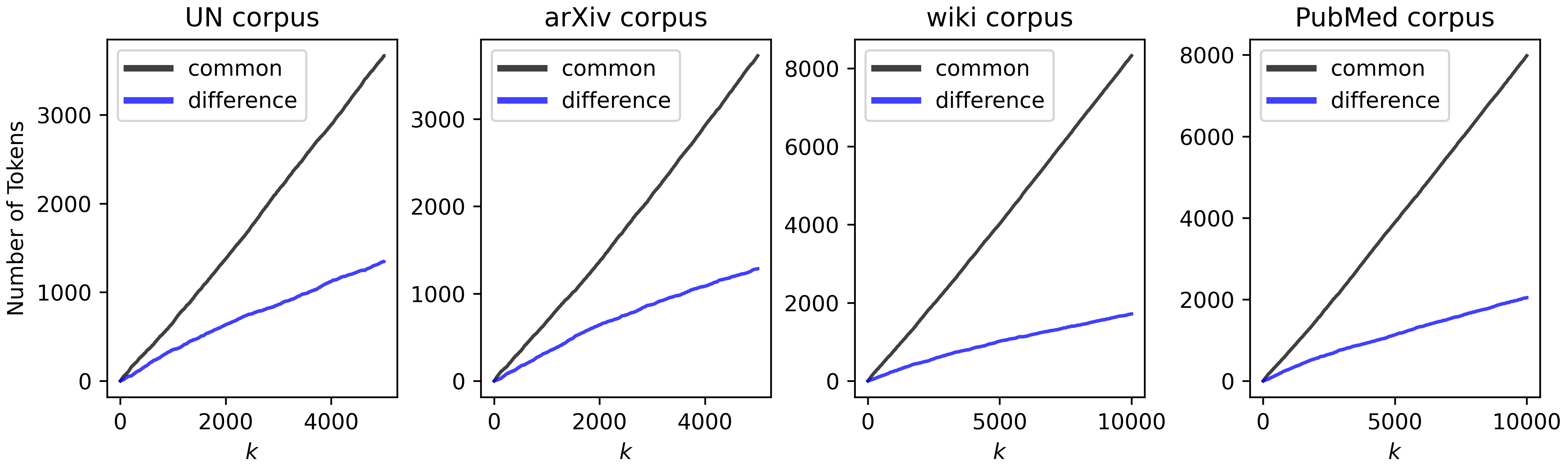
Figure 2: Plots showing constant rate of divergence of GreedTok and BPE algorithms in choice of tokens $\mathbf{S}$. The ordering in legend reflects the vertical ordering of the lines.

Qualitative findings.

From Table 3, to achieve the same tokens per word target, we see that GreedTok requires an average of 13% fewer tokens than BPE while using an average of 3%, and up to 5%, fewer tokens per word across various experimental settings; see the “Ratio of $k_{g}/k_{b}$” and “Ratio of $\textsc{GreedTok}(k_{g})/\textsc{BPE}(k_{g})$” rows respectively. Meanwhile, in Fig. 2, we observe a constant rate of divergence between the ranked token sequences $\mathbf{S}$ of GreedTok and BPE. Our findings show that GreedTok consistently uses a fewer number of tokens (including singletons) to encode the chosen corpora. This suggests that BPE’s pairwise merges may have prevented the selection of tokens with better compression utility.

5.3 Towards understanding GreedTok’s approximability

We reformulated Problem 1 into a MIP in Section 4.2 because the MIP formulation relaxes naturally into the maximum coverage problem, which has a corresponding $(1-1/e)$ approximate algorithm GreedWMC. By deploying GreedWMC on the same problem instances with the same range of $k$, we can calculate the ratio of objectives between GreedTok and GreedWMC and define $d_{\text{inst}}=\frac{\text{{GreedTok}}}{\text{{GreedWMC}}}$ for each instance. For each of these instances, GreedTok attains an objective value at least $d_{\text{inst}}(1-1/e)$ times the optimal objective of Eq. 1 by definition. This is because GreedWMC is an $(1-1/e)$-approximation algorithm to MWC, and GreedWMC’s attainable objective value of MWC is at least that of Tok; see Section 4.2.1.

Qualitative findings.

From Fig. 3, on the four selected corpora, we plot $d_{\text{inst}}$ against $k$. We see an initial steep decline before the curve reverses and climbs towards 1. At the start, the deviations suggest that GreedWMC selects tokens that partially overlap with each other, as a result GreedTok is unable to select these tokens as they will violate the MIP’s constraints. Fortunately, there is a turning point when the incremental gains of GreedTok outpace GreedWMC’s as $k$ increases. This suggests that singletons that were covered earlier by GreedWMC’s partially overlapping tokens would have eventually been covered by a single token assigned by GreedTok. Empirically, we see that GreedTok achieves an objective value of at least $0.9(1-1/e)$ of the optimal for large $k$, which is the case for practical NLP scenarios.

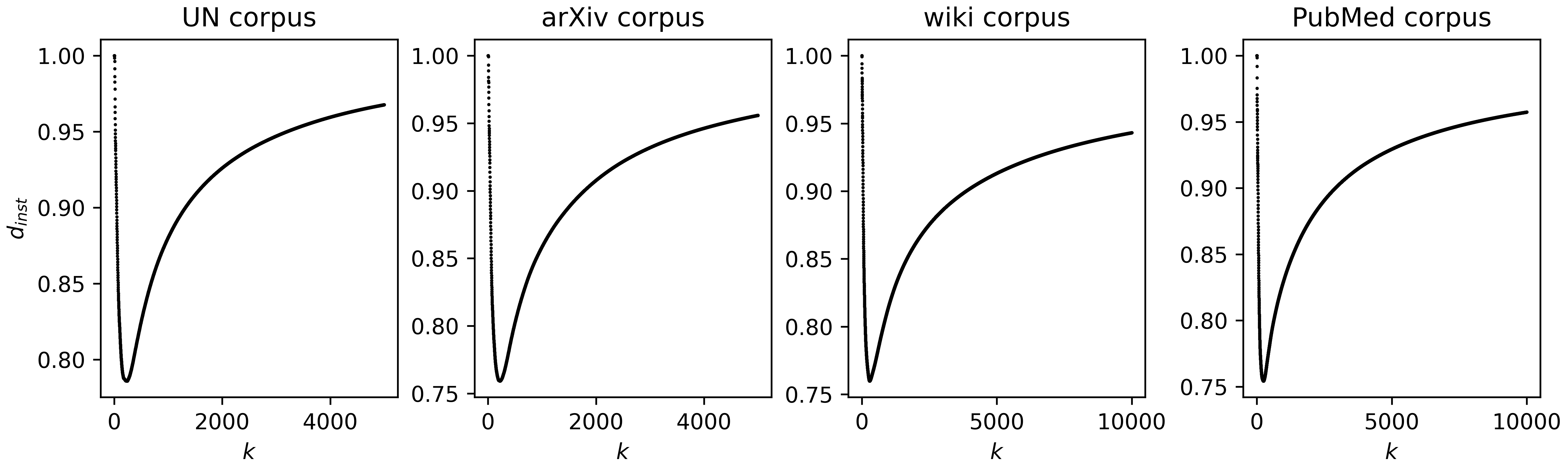
Figure 3: Plots showing exact $d_{\text{inst}}$ of each problem instance at different values of $|\mathbf{S}|=k$. As $k$ increases, the ratio of objectives $d_{\text{inst}}$ between $\textsc{GreedTok}(k)$ and $\textsc{GreedWMC}(k)$ closes.

5.4 Leveraging domain expertise in tokenization

Here, we discuss a new algorithmic design capability that is enabled by our general tokenization formulation.

For an extremely large corpus, considering all possible substrings for the candidate token set $\mathbf{T}$ may be daunting. However, if we had additional prior knowledge on how parts of the corpus differ, as a way to speed up the computation, we could run GreedTok on different subsets of the corpus and use the union of these outputs as the candidate token set $\mathbf{T}$ for the entire corpus. That is, one can leverage on domain expertise to cluster subsets of the corpus in order to generate these intermediate token sets $\mathbf{S}_{1},\ldots,\mathbf{S}_{K}$ and define $\mathbf{T}$ as all possible substrings of length at least 2 within $\mathbf{S}_{1},\ldots,\mathbf{S}_{K}$ instead of considering all possible substrings of length $\geq 2$ within $\mathbf{W}$ for the initial candidate set $\mathbf{T}$. This approach also allows one to incorporate selected tokens from other sources $\mathbf{S}_{\text{other}}$, such as outputs from other tokenization algorithms or domain experts, as we can simply consider $\mathbf{S}_{1}\cup\ldots\cup\mathbf{S}_{K}\cup\mathbf{S}_{\text{other}}$ when forming the input $\mathbf{T}$ for GreedTok.

As a concrete example, let us consider wiki-cjk, a corpus of articles from the Chinese, Japanese, and Korean (CJK) language sections of Wikipedia that contain CJK characters. First, we use GreedTok on each subset of articles belonging to the same language domain to obtain their respective local outputs $\mathbf{S}_{C},\mathbf{S}_{J},\mathbf{S}_{K}$, each of size $|\mathbf{S}|=k$, and then run GreedTok again with the candidate token set $\mathbf{T}$ as all possible substrings of length at least 2 within $\mathbf{S}_{C}\cup\mathbf{S}_{j}\cup\mathbf{S}_{K}$, on the full corpus counts to obtain the final output $\mathbf{S}_{CJK}$, where $|\mathbf{S}_{CJK}|=k$. Doing this pre-processing step reduces the size of the considered candidate set $|\mathbf{T}|$ from $320M$ to $231K$. Our experimental results are visualized in Fig. 4. Examining the three language subsets, using a $\mathbf{S}$ obtained from a foreign language to tokenize leads to subpar performance in terms of tokens per word, as evidenced in the two highest curves. Meanwhile, the tokenization performance of $\mathbf{S}_{CJK}$ only slightly trails the performance of the native tokenizer (e.g. $\mathbf{S}_{C}$ on wiki-chinese, $\mathbf{S}_{J}$ on wiki-japanese, and $\mathbf{S}_{K}$ on wiki-korean), indicating a successful combination of the three languages despite sacrificing some tokenization performance to accommodate all three language domains.

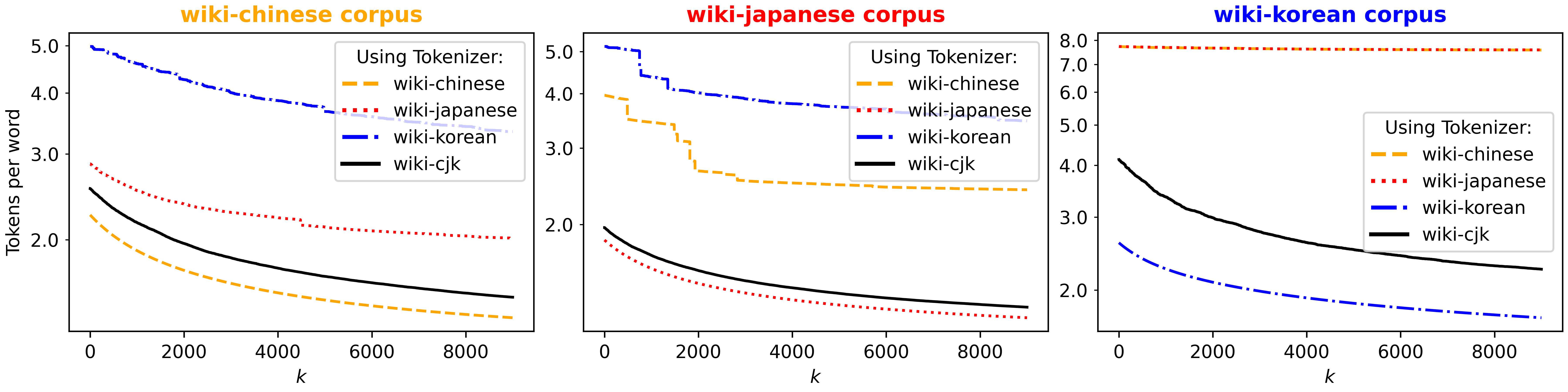
Figure 4: Plots of tokenizing different corpora using different local GreedTok sequences (lower is better). The sequence for wiki-cjk is obtained from the other three sequences, showing a successful combination.Y-axis is on a logarithmic scale. For the wiki-korean corpus, the curves from using $\mathbf{S}_{C}$ (wiki-chinese) and $\mathbf{S}_{J}$ (wiki-japanese) tokenizers overlaps. Observe that in each language domain, the native language tokenizer produces the lowest curve, with the combined $\mathbf{S}_{CJK}$ (wiki-cjk) trailing it, and the foreign language tokenizers having the worst performance. With the combined $\mathbf{S}_{CJK}$ outperforming the foreign language counterparts in the three language domains, it is suffice to conclude that the combination between $S_{C}$, $S_{J}$ and $S_{K}$ (wiki-korean) is a success.

5.4.1 Computational Feasibility

Table 4 details the total compute time for GreedTok to obtain $\mathbf{S}$, where $|\mathbf{S}|=\max k$, conducted with AMD EPYC 9654 @ 2.40GHz and 768 GB of RAM. If required, one can manually adjust $\max|W|$, $\mathbf{W}$, and $\mathbf{T}$ to reduce the search space of the solution. For example, one could ignore long words when building $\mathbf{T}$ to reduce $\max|W|$, ignore certain words when building $\mathbf{T}$ to reduce $|\mathbf{W}|$, or consider only substrings of longer length (or prune $\mathbf{T}$ in other ways) when building $\mathbf{T}$. To benchmark encoding performance, we encode using a token set of $|\mathbf{S}|=100$K, on a subset of wiki comprising 70K text articles with a total of 97M words. With a similar compute environment, our current initial implementation of GreedTok processes texts at a rate of 700K to 800K words per second per thread; we believe these numbers can be further optimized. With these performance characteristics, we believe that it is feasible to employ GreedTok in NLP pipelines.

Data	$\max k$	$\max|W|$	$|\mathbf{W}|$	$|\mathbf{T}|$	Total Time
UN	5K	71	105K	884K	2m 21s
ar$\chi$iv	5K	94	881K	7.6M	29m 13s
wiki	10K	333	8.7M	93.5M	12h 37m 26s
PubMed	10K	2,615	6.5M	121.1M	24h 52m 00s
wiki-chinese	10K	60	7.0M	69.7M	12h 42m 10s
wiki-japanese	10K	60	2.7M	60.4M	10h 31m 49s
wiki-korean	10K	60	5.4M	130.9M	25h 50m 11s
wiki-cjk	10K	60	14.2M	231K	3h 41m 36s

Table 4: The time taken for code execution. The first half contains experiments in Section 5.2 and Section 5.3, and the second half contains experiments in Section 5.4. Since the algorithms are deterministic, the results of one run is reported. For wiki-cjk and its subsets, we had a 20 CJK-character limit, i.e. 60 bytes.

6 Conclusion

In this work, we showed that the tokenization problem is NP-hard, provided a greedy algorithm GreedTok, and empirically demonstrated its edge over the incumbent BPE in terms of the compression utility metric. Our general formulation of the tokenization problem also enables the use of custom candidate token sets to search over and to leverage on domain expertise for learning specialized tokens for subsets of corpora. We hope that our formulation of the tokenization problem will be valuable for future research and we believe that substituting BPE with GreedTok as the tokenization algorithm is straightforward in almost all modern NLP systems. Below, we discuss some potential implications of our work and state a concrete open problem.

Towards a flexible algorithmic framework for tokenization.

BPE is a tokenization algorithm with widespread adoption currently. However, as shown and discussed in Section 5, GreedTok is a practical alternative that is more efficient in tokenization while enabling additional benefits of not relying on pairwise merge sequences. While the recent current advances in long-context research [HKM⁺24, GT24] seeking to enable a context length of a million tokens may make the compression utility metric a less important criterion in choosing a tokenization algorithm, our proposed MIP formulation and GreedTok offer a flexible platform to adapt to new alternate objectives that may arise in the future. For instance, our flexible formulation allows one to directly incorporate pre-selected tokens as part of the initial candidate token set $\mathbf{T}$; see also Section 5.4 for a concrete example of how these candidate tokens can be incorporated into $\mathbf{T}$. It would also be interesting future work to integrate NLP downstream objectives [BD20] and fairness [LBG⁺24] constraints into our MIP formulation.

Moving past pre-defined tokenizers.

Tokenizer-free architectures such as Charformer [TTR⁺22], ByT5 [XBC⁺22], MegaByte [YSF⁺23], and Byte Latent Transformers [PPR⁺24] avoid the use of tokenizers completely by using character or byte level information as opposed to fixed tokens. From our MIP, one can view the $0/1$ bits of $m^{W}$ as a sequential binary prediction problem of whether to merge adjacent characters of a word $W\in\mathbf{W}$. Given that modern LLMs have great empirical performance on next-token prediction, it would be interesting to see if one could leverage them in performing this sequential binary prediction task. This would effectively result in a tokenization algorithm that does not rely on a pre-defined initial candidate token set $\mathbf{T}$.

Open problem.

Recall that the tokenization problem has the confounding property of being neither supermodular nor submodular. Even though we empirically show that GreedTok achieves an approximation ratio of at least $0.9(1-1/e)$ for large $k$, a formal proof is lacking. This is an intriguing theoretical problem and we believe that our perspective of the tokenization problem may help in this future endeavor.

Appendix A Additional Pseudocode

Previously, in our MIP (Section 4.2), a 1-based indexing system was used. However, for implementation convenience, we use a 0-based indexing system for our pseudocodes instead. Given an ordered sequence $\mathcal{S}$, such as array $A$, string $W$, and selected tokens $\mathbf{S}$, we use $\mathcal{S}_{i}$ to specify an element in the $i^{th}$ index of $\mathcal{S}$. However, for sequences, we use $\mathcal{S}_{i,j}$ to specify the elements from the $i^{th}$ index up to, but excluding, the $j^{th}$ of $\mathcal{S}$. For example, when $\mathcal{S}=\text{happy}$, we have $\mathcal{S}_{1}=\text{a}$ and $\mathcal{S}_{1,3}=\text{ap}$.

A.1 Computing $\mathcal{S}$ from $\mathcal{T}$

Given the Count function, corpus $\mathbf{W}$, candidate tokens $\mathbf{T}$, and an integer $k$, Algorithm 1 finds a set of tokens $\mathbf{S}$ that maximizes the objective function with the help of subroutines Algorithm 2 and Algorithm 3. The algorithm Algorithm 1 defines a couple of dictionaries $\mathbf{M}$, $\mathbf{P}$, $\mathbf{R}$, and $\mathbf{I}$ to track the problem state, then greedily picks the next best scoring token to cover words:

1. $\mathbf{M}$ maps each word $W$ to its state of cover, similar to the definition in Section 4.2

2. $\mathbf{P}$ maps each token $T$ to the set of its occurrences in the given word $W$, for all $W\in\mathbf{W}$, in a ($W$, $i$) pair, where $i$ is the position index of the start of the token occurrence

3. $\mathbf{R}$ stores the net objective gain of each $T$, which we use to greedily select the next best token in LABEL:{lst:main:greedy_pick}

4. $\mathbf{I}$ maps each token $T$ to an index, which we use to update the state of cover for all $W\in\mathbf{W}$ at 14

The subroutine Algorithm 2 encapsulates a check of the validity of using a given token $T$ to cover $W$ at position $i$, primarily by observing if the non-start/end endpoint positions $i$ and $i+|T|$ were previously covered by some other token previously; if such a token is present, then $T$ cannot cover $W$ at position $i$. Meanwhile, the subroutine Algorithm 3 calculates the score contribution by token $T$, given the current state $\mathbf{M}$, while accounting for previous covers applied from chosen tokens in $\mathbf{S}$.

Algorithm 1 GreedTok: Computing $\mathbf{S}$

1:Count function, corpus words $\mathbf{W}$ where $|W|\geq 2$ for all $W\in\mathbf{W}$, candidate tokens $\mathbf{T}$, integer $k$

2:Initialize dictionary $\mathbf{M}:\mathbf{W}\to\mathbb{N}^{+}$ with $\triangleright$ State of the algorithm

$$\mathbf{M}(W)=(m^{W}_{0,1},\dots,m^{W}_{|W|-2,|W|-1})=(0,\ldots,0)=0^{|W|-1}\qquad\text{for all $W\in\mathbf{W}$}$$

3:Initialize dictionary $\mathbf{P}:\mathbf{T}\to(\mathbf{W}\times\mathbb{N})^{*}$ with $\mathbf{P}(T)=\{(W,i)\in\mathbf{W}\times\mathbf{N}:W_{i,i+|T|}=T\}$ for all $T\in\mathbf{T}$

4:$\triangleright$ Positioning information of tokens in words

5:Initialize dictionary $\mathbf{R}:\mathbf{T}\to\mathbb{N}$ with $\mathbf{R}(T)=0$ for all $T\in\mathbf{T}$ $\triangleright$ Token scores given current state

6:Initialize dictionary $\mathbf{I}:\mathbf{T}\to\mathbb{N}$ where $\mathbf{I}(T)=0$ for all $T\in\mathbf{T}$ $\triangleright$ Token indices in $\mathbf{S}$

7:Initialize $\mathbf{S}$ as an empty sequence

8:while $|\mathbf{S}|<k$ do

9:  Compute scores $\mathbf{R}(T)$ for each $T\in\mathbf{T}\setminus\mathbf{S}$ using Score on current state $\mathbf{M}$ $\triangleright$ Algorithm 3

10:  Greedily pick the next best token $\tau=\operatorname*{argmax}_{T\in\mathbf{T}}\mathbf{R}(T)$

11:  Append $\tau$ to the back of $\mathbf{S}$ and then update $\mathbf{I}(\tau)=|\mathbf{S}|$

12:  for $(W,i)\in\mathbf{P}(\tau)$ do $\triangleright$ Update states of $\mathbf{M}(\tau)$

13:   if $\textsc{CanCover}(\mathbf{M},\tau,W,i)$ then

14:     Update each entry of $\mathbf{M}(W)_{i,i+|\tau|-1}$ to $\mathbf{I}(\tau)$

15:   end if

16:  end for

17:end while

18:return $\mathbf{S}$

Algorithm 2 CanCover: Check if $W_{i,i+|T|-1}$ is coverable by $T$ in current state $\mathbf{M}$

1:Current state $\mathbf{M}$, token $T$, word $W$, position index $i$

2:return ($i=0$ or $\mathbf{M}(W)_{i-1}=0$) and ($i+|T|=|W|$ or $\mathbf{M}(W)_{i+|T|-1}=0$)

Algorithm 3 Score: Calculate total number of possible covers

1:Token $T$, token positions $\mathbf{P}(T)$, current state $\mathbf{M}$, count function

2:Make a copy $\mathbf{M}^{\prime}$ of the state $\mathbf{M}$ $\triangleright$ The original state remains unchanged

3:Initialize token score $s=0$

4:for $(W,i)\in\mathbf{P}(T)$ do

5:  if $\textsc{CanCover}(\mathbf{M}^{\prime},T,W,i)$ then

6:   Add $\textsc{count}(W)\cdot|\{j\in\{i,\ldots,i+|T|\}:\mathbf{M}^{\prime}(W)_{j}=0\}|$ to $s$ $\triangleright$ Only add score for non-zero entries

7:   Update each entry of $\mathbf{M}^{\prime}(W)_{i,i+|T|-1}$ to $1$ $\triangleright$ Mark to avoid double counting; see Example 5

8:  end if

9:end for

10:return $s$

Example 4 (Valid coverings and two sample traces).

Consider the example where $\mathbf{T}=\{T_{1}=\text{pa},T_{2}=\text{ya},T_{3}=\text{ap}\}$ and $\mathbf{W}=\{W_{1}=\text{papaya},W_{2}=\text{impact}\}$. Then, we have $\mathbf{P}(T_{1})=\{(W_{1},0),(W_{1},2),(W_{2},2)\}$, indicating that the token $T_{1}$ appears in $W_{1}$ at positions $0$ and $2$, and in $W_{2}$ at position $2$. Using Score (Algorithm 3) to update $\mathbf{R}$ would yield $\mathbf{R}(\text{pa})=3$, $\mathbf{R}(\text{ya})=1$, and $\mathbf{R}(\text{ap})=1$, so the greedy step 10 of Algorithm 1 would first select token $T_{1}$ to be included into $\mathbf{S}$. Initially, we have $\mathbf{M}(W_{1}=\text{papaya})=(0,0,0,0,0)$. After selecting $T_{1}$ into $\mathbf{S}$, we have $\mathbf{M}(W_{1})=(1,0,1,0,0)$. Recalculating the scores using Score on the updated state $\mathbf{M}$ would yield $\mathbf{R}(\text{pa})=0$, $\mathbf{R}(\text{ya})=1$, and $\mathbf{R}(\text{ap})=0$, so the token $T_{2}$ would be selected next. After selecting $T_{2}$ into $\mathbf{S}$, we have $\mathbf{M}(W_{1})=(1,0,1,0,2)$ because $\mathbf{I}(T_{1}=\text{pa})=1$ and $\mathbf{I}(T_{2}=\text{ya})=2$. One can see that the zero and non-zero locations in $\mathbf{M}$ indicate partition and coverage respectively. Now, ignoring the scoring function, let us instead suppose that we selected $T_{3}=\text{ap}$, $T_{1}=\text{pa}$, and finally $T_{2}=\text{ya}$. When we first selected $T_{3}=\text{ap}$, the state of $W_{1}=\text{papaya}$ will become $M(W_{1})=(0,1,0,0,0)$ with $\mathbf{I}(T_{3}=\text{ap})=1$. Next, consider the token $T_{1}=\text{pa}$ that appears at positions $0$ and $2$ of the word $W_{1}$. At position $0$, we see that $\mathbf{M}(W_{1})_{i+|T|-1=0+2-1=1}=1\neq 0$. Meanwhile, at position 2, we have $\mathbf{M}(W_{1})_{i-1=2-1}=1\neq 0$. Since there is at least one non-start/end endpoint positions already covered by a token, we cannot further use $T_{1}$ in $W_{1}$. Finally, let us consider using token $T_{2}=\text{ya}$, which appears at position 4 of $W_{1}$. We see that $i>0$, $\mathbf{M}(W_{1})_{i-1}=0$, and $i+|T_{2}|<|W_{1}|$, we can cover $W_{1}$ with $T_{2}$ at position 4, resulting in $M(W_{1})=(0,1,0,0,2)$ with $\mathbf{I}(\text{ya})=2$. Note that we do not need to check $\mathbf{M}(W_{1})_{i+|T_{2}|-1}$ because $i+|T_{2}|<|W_{1}|$.

Example 5 (State copying and overcounting).

Here, we explain why we require a copy of the state in Algorithm 3 to avoid the overcounting of overlapping repeating substrings. Consider the example of $T_{1}=\text{aya}$, $W_{1}=\text{ayaya}$, and $\textsc{count}(W_{1})=1$, where $\mathbf{P}(T_{1})=\{(W_{1},0),(W_{1},2)\}$ and $\mathbf{M}(W_{1})=\mathbf{M}^{\prime}(W_{1})=(0,0,0,0)$ initially. In this case, we see that $T_{1}$ would obtain a score of 1 either by covering $W_{1}$ at position 0 (i.e. ayaya) or position 2 (i.e. ayaya), but not both positions simultaneously (i.e. ayaya). To see how Algorithm 3 ensures this, let us suppose we considered $(W_{1},0)$ then $(W_{1},2)$ in the for loop iteration. As the endpoints of $(W_{1},0)$ are coverable, we update $\mathbf{M}^{\prime}(W_{1})$ to $(1,1,0,0)$. Note that $\mathbf{M}(W_{1})$ still remains unchanged as we have yet to confirm that $T_{1}$ is the next best token $\tau$. With the updated state $\mathbf{M}^{\prime}$, we see that the next pair $(W_{1},2)\in\mathbf{P}(T_{1})$ is an invalid cover since $\mathbf{M}^{\prime}(W_{1})_{2-1=1}=1\neq 0$, which prevents an overcounting. We remark that the choice of updating entries to $1$ is arbitrary (i.e. any non-zero value will work) and that one can actually avoid explicitly making a copy of the state in implementation by performing checks in an appropriate manner.

Runtime complexity for computing $\mathcal{S}$.

Each call to CanCover (Algorithm 2) runs in $O(1)$ time. Fix an arbitrary iteration of the while loop in Algorithm 1. Each call to Score (Algorithm 3) with token $T$ runs in $O(\sum_{W\in\mathbf{W}}|W|)$ time because it iterates through each position in $\mathbf{P}(T)$ once and considers if $T$ is a valid cover for that position. While we update $\mathbf{M}(W)$ during the iteration, due to CanCover (Algorithm 2), each index is updated at most once to a non-zero value, i.e. Example 5, resulting in at most $O(\sum_{W\in\mathbf{W}}|W|)$ total number of updates. Therefore, applied across all tokens $T\in\mathbf{T}$, $k$ number of times, Algorithm 1 takes $O(|\mathbf{T}|\cdot k\cdot\sum_{W\in\mathbf{W}}|W|)$ time to compute $\mathcal{S}$.

Additional implementation remarks.

In practice, it is possible to adopt alternative data representations. For example, instead of a dictionary, one could represent $\mathbf{M}$ as a single contiguous array and define a given word $W$ as a position in the array. One could also use a representation of length $|W|$ for each word instead of the $(|W|-1)$-sized representation discussed in 2 and Section 4.2. For example, covering the word $W=\text{papaya}$ by token $T_{1}=\text{pa}$ could be represented by $(1,1,1,1,0,0)$ instead of $(1,0,1,0,0)$. However, in the $(1,1,1,1,0,0)$ representation, it is impossible to discern a partition and one has to keep track of additional information regarding duplicates of tokens within the same word. Furthermore, one can avoid redundant calculations of $\mathbf{P}$ by tracking and only recalculating the affected $T$ in words covered by the current $\tau$.

A.2 Tokenizing a text $W$ using $\mathcal{S}$

In Algorithm 4, we describe how to encode a given text $W$ into its token representation using the token set $\mathbf{S}$ from Algorithm 1. First, in 2, we initialize a dictionary to map our tokens in $\mathbf{S}$ according to their order of inclusion to $\mathbf{S}$, and then place singleton tokens $\mathbf{B}$ at the back of the sequence. Next, in 3, we find all possible token covers of $W$ using tokens in $\mathbf{S}$ and sort them in 4 according to their priority $\mathbf{I}$ and a left-to-right ordering in $W$. Using $\mathbf{M}$ to denote which token covers which position index of $W$, we iterate through $(T,i)$ in the sorted $\mathbf{P}$ and update $\mathbf{M}$ whenever the token $T$ can cover $W$ at position $i$ given earlier decisions. Note that this may mean that a later token of longer length may overwrite the covering decision of an earlier shorter token; see Example 6. Finally, using $\mathbf{M}$, we return the 0-delineated token representation; see Example 7.

Algorithm 4 GreedTok: Tokenizing a given text $W$ using $\mathbf{S}$

1:Text $W$, singleton tokens $\mathbf{B}$, chosen token sequence $\mathbf{S}$

2:Initialize dictionary $\mathbf{I}:\mathbf{S}\cup\mathbf{B}\to\mathbb{N}$ with

$$\mathbf{I}(T)=\begin{cases}i&\text{if $T$ is $i^{th}$ chosen token in $\mathbf{S}$}\\ |\mathbf{S}|+i&\text{if $T$ is $i^{th}$ token in $\mathbf{B}$}\end{cases}$$

$\triangleright$ Fix an arbitrary ordering to singleton tokens

3:Initialize potential cover positions $\mathbf{P}=\{(T,i):T\in\mathbf{S},W_{i,i+|T|}=T\}$

4:Sort $\mathbf{P}$ based on $\mathbf{I}(T)$, then position $i$, with lower values having greater priority

5:Initialize state $\mathbf{M}=\{m_{0,1},\dots,m_{|W|-2,|W|-1}\}=0^{|W|-1}$

6:for $(T,i)\in\mathbf{P}$ in descending sorted order of 4 do

7:  if $\textsc{CanCover}(\mathbf{M},T,W,i)$ then

8:   Update each entry of $\mathbf{M}_{i,i+|T|-1}$ to $\mathbf{I}(T)$

9:  end if

10:end for

11:return $W$ delineated at positions of $0$ $\triangleright$ See Example 7

Example 6 (Overriding earlier shorter tokens).

Consider the encoding of $W_{1}=\text{abcdefg}$ with $\mathbf{S}=(S_{1}=\text{ab},S_{2}=\text{cd},S_{3}=\text{ef},S_{4}=\text{abc},S_{5}=\text{abcd},S_{6}=\text{efg},S_{7}=\text{abcdefg})$. In the first three iterations, we use $S_{1}$, $S_{2}$, and $S_{3}$ to cover $W$, resulting in $\mathbf{M}=(1,0,2,0,3,0)$. Then, we see that $S_{4}$ does not have any valid covers and so $\mathbf{M}$ remains unchanged. In the fifth and sixth iterations, notice that $S_{1},S_{2}\subset S_{5}$ and $S_{3}\subset S_{6}$, resulting in $S_{5}$ and $S_{6}$ being valid covers and $\mathbf{M}$ being updated to $(5,5,5,0,6,6)$. Finally, since $S_{5},S_{6}\subset S_{7}$ and $S_{7}$ is a valid cover with respect to the current state, $\mathbf{M}$ becomes $(7,7,7,7,7,7)$. Now, consider another scenario of encoding $W_{2}=\text{abcd}$ using $\mathbf{S}=(S_{8}=\text{ab},S_{9}=\text{abc},S_{10}=\text{abcd})$, where $S_{8}\subset S_{9}\subset S_{10}$. Covering $W_{2}$ using $S_{8}$ results in $\mathbf{M}=(1,0,0)$. Then, using $S_{9}$ results in $\mathbf{M}=(2,2,0)$. Finally, using $S_{10}$ results in $\mathbf{M}=(3,3,3)$. In both examples, we see that covers are only overridden by proper supersets that appear later in the ordering of $\mathbf{S}$, where the largest valid cover in $\mathbf{S}$ for $W$ is of size $|W|$. Furthermore, recall that the token covers of any valid covering do not overlap so they jointly take up at most $|W|$ positions in total. As such, we see that each position $\mathbf{M}_{i}\in\mathbf{M}$ is updated at most $|W|$ times and thus, across all $|W|$ positions, Algorithm 3 updates values in $\mathbf{M}$ a maximum of $O(|W|^{2})$ times.

Example 7 (Encoding the tokenized output).

If $W=\text{abcdef}$, $\mathbf{S}=\{S_{1}=\text{bcd},S_{2}=\text{ef}\}$ and $\mathbf{M}=(0,1,1,0,2)$, then $W$’s final tokenized output will be $(\text{a},\text{bcd},\text{ef})$. If one wishes to convert the tokens to integers with respect to token indexing, simply apply $\mathbf{I}$ to each token to get $(\mathbf{I}(\text{a}),\mathbf{I}(\text{bcd}),\mathbf{I}(\text{ef}))$.

Runtime complexity for tokenizing $W$ using $\mathcal{S}$.

Each call to CanCover (Algorithm 2) runs in $O(1)$ time. There are at most $\binom{|W|}{2}\in O(|W|^{2})$ substrings of $W$ and so 3 runs in $O(|W|^{2})$ time, $|\mathbf{P}|\in O(|W|^{2})$ and sorting $\mathbf{P}$ takes $O(|W|^{2}\log(|W|)$ time. Since each index can only be overwritten when a longer token covers it, in 8, we see that each position in $\mathbf{M}$ is only updated at most $|W|$ times, and therefore a maximum of $|W|^{2}$ for all positions in $|\mathbf{P}|$ number of iterations; see Example 6. Thus, the entire for loop takes $O(|\mathbf{P}|+|W|^{2})\subseteq O(|W|^{2})$ time to iterate through $\mathbf{P}$ and to update all $O(|W|)$ positions in $\mathbf{M}$.

Additional implementation remarks.

In practice, we limit the subsequence search to the maximum token length $\ell=\max_{T\in\mathbf{S}}|T|$, with early stopping. To reduce $|W|$ even further, we have to go beyond regex and identify smaller local sections within $W$ so that we can independently tokenize these sections. This is possible as $\mathbf{S}$ inadvertently learns the regex pattern and more during its construction. This implies that we can also further infer natural separations within $W$ where no $T\in\mathbf{S}$ overlaps with another.

References

- [Att15] Giusepppe Attardi. Wikiextractor. https://github.com/attardi/wikiextractor, 2015.
- [BD20] Kaj Bostrom and Greg Durrett. Byte Pair Encoding is Suboptimal for Language Model Pretraining. In Findings of the Association for Computational Linguistics: EMNLP 2020, pages 4617–4624, 2020.
- [CK08] Reuven Cohen and Liran Katzir. The generalized maximum coverage problem. Information Processing Letters, 108(1):15–22, 2008.
- [CLL+05] Moses Charikar, Eric Lehman, Ding Liu, Rina Panigrahy, Manoj Prabhakaran, Amit Sahai, and Abhi Shelat. The smallest grammar problem. IEEE Transactions on Information Theory, 51(7):2554–2576, 2005.
- [FTL+23] Caoyun Fan, Jidong Tian, Yitian Li, Wenqing Chen, Hao He, and Yaohui Jin. Chain-of-Thought Tuning: Masked Language Models can also Think Step By Step in Natural Language Understanding. In Conference on Empirical Methods in Natural Language Processing (EMNLP), pages 14774–14785, 2023.
- [Gag94] Philip Gage. A new algorithm for data compression. The C Users Journal, 12(2):23–38, 1994.
- [GT24] Google Gemini Team. Gemini 1.5: Unlocking multimodal understanding across millions of tokens of context. arXiv preprint arXiv:2403.05530, 2024.
- [HKM+24] Coleman Hooper, Sehoon Kim, Hiva Mohammadzadeh, Michael W. Mahoney, Yakun Sophia Shao, Kurt Keutzer, and Amir Gholami. KVQuant: Towards 10 Million Context Length LLM Inference with KV Cache Quantization. In Advances in Neural Information Processing Systems (NeurIPS), 2024.
- [Hoc96] Dorit S. Hochbaum. Approximating covering and packing problems: set cover, vertex cover, independent set, and related problems. In Approximation algorithms for NP-hard problems, pages 94–143. PWS Publishing Co., 1996.
- [JBD17] Slava Jankin, Alexander Baturo, and Niheer Dasandi. United Nations General Debate Corpus 1946-2023. https://doi.org/10.7910/DVN/0TJX8Y, 2017.
- [JSM+23] Albert Q Jiang, Alexandre Sablayrolles, Arthur Mensch, Chris Bamford, Devendra Singh Chaplot, Diego de las Casas, Florian Bressand, Gianna Lengyel, Guillaume Lample, Lucile Saulnier, et al. Mistral 7B. arXiv preprint arXiv:2310.06825, 2023.
- [Kar72] Richard M. Karp. Reducibility among Combinatorial Problems. In Complexity of Computer Computations, pages 85–103. Springer, 1972.
- [KHM+23] Jean Kaddour, Joshua Harris, Maximilian Mozes, Herbie Bradley, Roberta Raileanu, and Robert McHardy. Challenges and applications of large language models. arXiv preprint arXiv:2307.10169, 2023.
- [Kud18] Taku Kudo. Subword regularization: Improving neural network translation models with multiple subword candidates. In Proceedings of the 56th Annual Meeting of the Association for Computational Linguistics (Volume 1: Long Papers), pages 66–75, 2018.
- [KV24] László Kozma and Johannes Voderholzer. Theoretical Analysis of Byte-Pair Encoding. arXiv preprint arXiv:2411.08671, 2024.
- [LBG+24] Tomasz Limisiewicz, Terra Blevins, Hila Gonen, Orevaoghene Ahia, and Luke Zettlemoyer. MYTE: Morphology-Driven Byte Encoding for Better and Fairer Multilingual Language Modeling. In Proceedings of the 62nd Annual Meeting of the Association for Computational Linguistics (Volume 1: Long Papers), pages 15059–15076, 2024.
- [LBM23] Tomasz Limisiewicz, Jiří Balhar, and David Mareček. Tokenization Impacts Multilingual Language Modeling: Assessing Vocabulary Allocation and Overlap Across Languages. In Findings of the Association for Computational Linguistics: ACL, 2023.
- [LXZ+19] Ruixuan Luo, Jingjing Xu, Yi Zhang, Zhiyuan Zhang, Xuancheng Ren, and Xu Sun. PKUSEG: A Toolkit for Multi-Domain Chinese Word Segmentation. arXiv preprint arXiv:1906.11455, 2019.
- [MHB+23] Ines Montani, Matthew Honnibal, Adriane Boyd, Sofie Van Landeghem, and Henning Peters. explosion/spaCy: v3.7.2: Fixes for APIs and requirements, 2023.
- [NWF78] G. L. Nemhauser, L. A. Wolsey, and M. L. Fisher. An analysis of approximations for maximizing submodular set functions–I. Mathematical Programming, 14(1):265–294, 1978.
- [Ope23] OpenAI. tiktoken. https://github.com/openai/tiktoken, 2023.
- [PPR+24] Artidoro Pagnoni, Ram Pasunuru, Pedro Rodriguez, John Nguyen, Benjamin Muller, Margaret Li, Chunting Zhou, Lili Yu, Jason Weston, Luke Zettlemoyer, et al. Byte Latent Transformer: Patches Scale Better Than Tokens. arXiv preprint arXiv:2412.09871, 2024.
- [PY88] Christos Papadimitriou and Mihalis Yannakakis. Optimization, approximation, and complexity classes. In Symposium on Theory of Computing (STOC), pages 229–234. Association for Computing Machinery (ACM), 1988.
- [SFWN23] Jimin Sun, Patrick Fernandes, Xinyi Wang, and Graham Neubig. A Multi-dimensional Evaluation of Tokenizer-free Multilingual Pretrained Models. In Findings of the Association for Computational Linguistics: EACL, 2023.
- [SHB16] Rico Sennrich, Barry Haddow, and Alexandra Birch. Neural Machine Translation of Rare Words with Subword Units. In Proceedings of the 54th Annual Meeting of the Association for Computational Linguistics (Volume 1: Long Papers), pages 1715–1725, 2016.
- [THK+18] Kazuma Takaoka, Sorami Hisamoto, Noriko Kawahara, Miho Sakamoto, Yoshitaka Uchida, and Yuji Matsumoto. Sudachi: A Japanese tokenizer for business. In Proceedings of the Eleventh International Conference on Language Resources and Evaluation (LREC 2018), 2018.
- [TLI+23] Hugo Touvron, Thibaut Lavril, Gautier Izacard, Xavier Martinet, Marie-Anne Lachaux, Timothée Lacroix, Baptiste Rozière, Naman Goyal, Eric Hambro, Faisal Azhar, et al. Llama: Open and efficient foundation language models. arXiv preprint arXiv:2302.13971, 2023.
- [TTR+22] Yi Tay, Vinh Q. Tran, Sebastian Ruder, Jai Gupta, Hyung Won Chung, Dara Bahri, Zhen Qin, Simon Baumgartner, Cong Yu, and Donald Metzler. Charformer: Fast character transformers via gradient-based subword tokenization. In International Conference on Learning Representations (ICLR), 2022.
- [WBP24] Philip Whittington, Gregor Bachmann, and Tiago Pimentel. Tokenisation is NP-Complete. arXiv preprint arXiv:2412.15210, 2024.
- [WS11] David P. Williamson and David B. Shmoys. The Design of Approximation Algorithms. Cambridge University Press, 2011.
- [WWS+22] Jason Wei, Xuezhi Wang, Dale Schuurmans, Maarten Bosma, Brian Ichter, Fei Xia, Ed H. Chi, Quoc V. Le, and Denny Zhou. Chain-of-Thought Prompting Elicits Reasoning in Large Language Models. In Advances in Neural Information Processing Systems (NeurIPS), pages 24824–24837, 2022.
- [XBC+22] Linting Xue, Aditya Barua, Noah Constant, Rami Al-Rfou, Sharan Narang, Mihir Kale, Adam Roberts, and Colin Raffel. ByT5: Towards a token-free future with pre-trained byte-to-byte models. Transactions of the Association for Computational Linguistics, 10:291–306, 2022.
- [YSF+23] Lili Yu, Dániel Simig, Colin Flaherty, Armen Aghajanyan, Luke Zettlemoyer, and Mike Lewis. MEGABYTE: modeling million-byte sequences with multiscale transformers. In Advances in Neural Information Processing Systems (NeurIPS), pages 78808–78823, 2023.
- [YYZ+23] Shunyu Yao, Dian Yu, Jeffrey Zhao, Izhak Shafran, Thomas L. Griffiths, Yuan Cao, and Karthik Narasimhan. Tree of Thoughts: Deliberate Problem Solving with Large Language Models. In Advances in Neural Information Processing Systems (NeurIPS), pages 11809–11822, 2023.
- [ZMG+23] Vilém Zouhar, Clara Isabel Meister, Juan Luis Gastaldi, Li Du, Tim Vieira, Mrinmaya Sachan, and Ryan Cotterell. A Formal Perspective on Byte-Pair Encoding. In Findings of the Association for Computational Linguistics: ACL 2023, pages 598–614. Association for Computational Linguistics, 2023.