Forecasting Anonymized Electricity Load Profiles
Abstract
In the evolving landscape of data privacy, the anonymization of electric load profiles has become a critical issue, especially with the enforcement of the General Data Protection Regulation (GDPR) in Europe. These electric load profiles, which are essential datasets in the energy industry, are classified as personal behavioral data, necessitating stringent protective measures. This article explores the implications of this classification, the importance of data anonymization, and the potential of forecasting using microaggregated data. The findings underscore that effective anonymization techniques, such as microaggregation, do not compromise the performance of forecasting models under certain conditions (i.e., forecasting aggregated). In such an aggregated level, microaggregated data maintains high levels of utility, with minimal impact on forecasting accuracy. The implications for the energy sector are profound, suggesting that privacy-preserving data practices can be integrated into smart metering technology applications without hindering their effectiveness.
Index Terms:
Data Anonymization, Electric Load Profiles, Load forecasting, Microaggregation.I Introduction
In early 2009, the European Commission, through Directive 2009/72/EC, mandated the widespread deployment of smart meters across Europe [1]. These devices are key in the digitalization of the energy sector [2], allowing automatic granular recording of energy consumption, covering electricity, natural gas, district heating and water use. In the electricity sector, smart meters typically record consumption data at a 15-minute resolution, generating what are known as load profiles. These devices also facilitate remote data transmission to the designated Distribution System Operator (DSO), which subsequently shares the data with energy suppliers. Smart meters load profiles play a critical role for DSOs and energy suppliers, as they are essential for tasks such as congestion management, peak load analysis, and consumption forecasting [3]. For energy suppliers, these profiles have become particularly valuable for understanding the evolving consumption behaviors of customers, driven by the increasing integration of Renewable Energy Resources (RES), such as photovoltaic systems and batteries, as well as the adoption of new electric technologies like Electric Vehicle (EV).
Despite the clear advantages of smart meters—such as automated, remote data collection and enhanced granularity [4]—their use faces significant challenges within the European Union. One major constraint arises from the General Data Protection Regulation (GDPR) [5], which has been in force since May 25, 2018. Under the GDPR, explicit user consent is required to process load profile data. Another constraint stems from the high granularity of smart meter data. As the resolution increases from hourly values to 15-minute intervals, 5-minute intervals, or even real-time data, it becomes possible to infer sensitive details about consumers’ lifestyles, daily routines, and home occupancy patterns. These combined challenges make it difficult to utilize smart meter data for third-party applications or even for energy suppliers, as GDPR imposes stringent measures to safeguard personal data, and consumers may hesitate to consent to the use of their granular load profiles for tasks like forecasting.
One potential solution to these constraints is pseudo-anonymization, which involves removing personal and quasi-identifiable information from smart meter data [6]. Since pseudonymization preserves consumer profiles intact, information regarding the consumers can still be accessed, presenting notable challenges to privacy. In summary, fully anonymizing data presents difficulties since energy consumption is intrinsically time-dependent, and mere removal of identifiers does not guarantee data anonymization.
The nature of time series in which the values at time are closely related to the ones at and reflects sequential and temporal dependencies. This characteristic limits the effectiveness of classical anonymization techniques based on data perturbations or shuffling, leaving non-perturbative techniques as viable alternatives [7].
Non-perturbative anonymization methods, however, come with trade-offs. As the level of anonymization increases, the utility of the data typically diminishes [8]. Reduced data utility can adversely impact forecasting capabilities, making it more challenging for energy suppliers to balance supply and demand or to accurately predict consumption patterns.
In this paper, we examine the impact of a specific non-perturbative anonymization method, microaggregation, on the accuracy of energy demand forecasting, particularly for the Short-Term Load Forecasting (STLF) with a one hour horizon. Microaggregation groups similar data points to obscure individual identities while preserving key dataset properties. Our analysis focuses on assessing how microaggregation affects the accuracy of energy demand forecasts. Results indicate that microaggregated data has minimal impact on forecasting accuracy at an aggregated level. This finding is significant, as it demonstrates that high levels of data utility can be maintained while ensuring user privacy. It allows energy suppliers and third parties, for instance, under project or service agreements, to work together to utilize smart meter data without direct user consent while remaining compliant with GDPR, safeguarding individual privacy, and retaining data utility.
II Background
II-A Dataset
In our study, we used a dataset from the Low Carbon London project, conducted by UK Power Networks between November 2011 and February 2014 in the London area [9]. This dataset, which records household electrical consumption in kilowatt-hours (kWh) at half-hour intervals, served as the foundation for our simulations.
The original dataset comprised more than 4000 households with electric measurements in half-hour resolution from 1st of January 2013 until 31st of December 2013. We selected a random sample of 1000 households from the original dataset to limit the computational requirements of the experiments.
II-B Anonymization
In the context of anonymizing electric load data, the focus resides on time series, specifically the measurement time (when) and the value (what). Other features, such as name, surname, Id, network, and additional attributes, are excluded from consideration. This results in a simplified dual tuple (when, what), where each element alone is insufficient for identification. However, when these tuples are analyzed as a time series, they can still enable the identification of consumers. Consequently, this data remains personal information and necessitates anonymization for third-party use.
There are various techniques for data anonymization, each offering different levels of robustness. These techniques fall into two main categories: generalization, which does not alter the data but reduces detail, and perturbation which modifies the data by replacing it with other values.
Given the temporal nature and the limitations it imposes, like not distorting time-dependent patterns or applying noise that could affect forecasting. We restricted ourselves to generalization methods such as k-anonymity and microaggregation.
K-anonymity[10], a technique within generalization, aims to prevent a data subject from being singled out by grouping them with at least other individuals. This is achieved by generalizing attribute values so that each individual shares the same value. For example, individual households’ consumption values are aggregated with those of other individuals and averaged, making the output indistinguishable from the outside.
In a different manner, in 2005, Jossep Domingo-Ferrer and Vicenç Torra [7] published an evolution to K-anonymity named Microaggregation. Their algorithm create based on simulart and not randomly groups of size . Their algorithm named Maximum Distance to Average Vector (MDAV) is as follows:
Recent research underscores that microaggregation alone may not be sufficient to fully protect smart grid data from disclosure risks. To address this, the DFTMicroagg algorithm was proposed, offering a dual-level perturbation mechanism to enhance privacy in energy systems [11]
The algorithm leverages the benefits of Discrete Fourier Transform (DFT) and microaggregation to provide an additional layer of protection. The DFTMicroagg algorithm first applies a low-pass filtering step using DFT to anonymize the data before applying the MDAV microaggregation.
Although the DFTMicroagg algorithm offers enhanced privacy protection by combining DFT with microaggregation, we decided not to use it due to its complexity and potential impact on data utility. The dual-level perturbation could introduce distortions that affect the accuracy of forecasting models.
To this end, we focused on simpler generalization methods like MDAV to achieve a balance between privacy and utility.
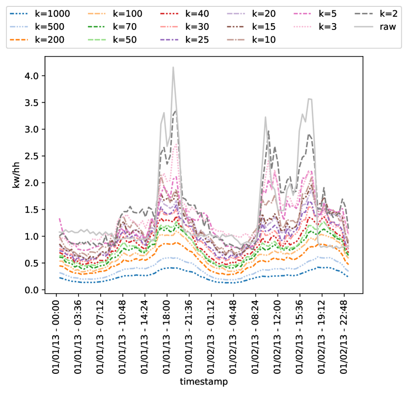
Figure1 represents one day of consumption for a given household and the groups the household is part of under different levels of anonymization.
II-C Forecasting
To forecast household electrical consumption and evaluate model performance under varying privacy levels, we compared different models, which we split into four groups: 1) baseline approaches, 2) statistical models, 3) machine learning (ML) models, and 4) neural network (NN) architectures. The baseline approach served as a reference point for evaluating other models. For statistical models, we selected MSTL[12] and MFLES[13]. Our ML models included XGBoost[14] and LGBM[15]. Lastly, we employed six NN architectures divided in two subcategories. Firstly the MLP-based models 111Referred as NN from now on in the paper.: MLP, NBEATS[16] and NHITS[17] and the transformer-based models: Autoformer[18], Informer[19], TFT[20].
Each category of models was configured differently. For the statistical models, we used the statsforecast library, setting the seasonal length to 48 as the data is in half-hour resolution, which corresponds to one day in half-hour resolution. Specifically, for MSTL, we incorporated AutoARIMA as it requires a seasonal forecaster.
For the ML models, we utilized the mlforecast library. We accounted for seasonality by including lags of 1, 48, and 336 being those previous half-hour, previous day and previous week. These lags were further transformed using Expanding Mean and Rolling Mean with a window size of 24. We also differentiated the target values with lags of 48 and 336, representing one day and one week, respectively. Additionally, we included the day of the week as an exogenous feature.
For the NN models, we employed the neuralforecast library. We set the local scaler to be robust to outliers using a robust local scaler. To manage computational demands, we empirically set the input size to 500 values.
This structured approach allowed us to systematically evaluate the trade-offs between data privacy and forecasting accuracy across different modeling techniques.
II-D Simulation Environment
We performed the simulations in the IRIS Cluster of the high-performance computer (HPC) facilities of the University of Luxembourg [21]. The simulations for the microaggregation ran in a specific node with 1 Tb of RAM while the forecasting models trained on one NVIDIA Tesla V100 with 16 Gb or 32 Gb depending on the allocation. We programmed the forecasting using the Nixtla stack [22, 23].
II-E Simulation Procedure
To evaluate the impact of on forecasting, we generated anonymized data sets by applying micro-aggregation to the original dataset. We defined nine levels of privacy as: , , , , , , , , , , , , , , .
With this, we created a set of different datasets with 500 the least private case () to 1 single group in the most private scenario with as an extreme case. This last group is equivalent to averaging all the profiles into a unique time series. In the opposite scenario, we keep the data without anonymization under the label raw in the upcoming experiments.
To evaluate the forecasting performance at different times in the year on the anonymized datasets and non-anonymized data, we employed a cross-validation approach. To minimize computational load, the forecasting process was divided into 5 stages or windows: (1) training on data up to August 28th and forecasting for August 29th, (2) training on data up to September 28th and forecasting for September 29th, (3) training on data up to October 29th and forecasting for October 30th. In the (4) stage, we train up to the 29th of November and forecast on the 30th, and lastly in (5) we train up to the 30th of December and forecast on the 31st. For each of the windows, the model retrains again to account for the new data. We then produce day-ahead forecasts; meaning we forecast 24 hours in advance. Since the dataset is in half-hour resolution, we forecast 48 values.
Once individual households or groups are forecasted, we aggregated them; in the raw case by simply summing across the households for a given timestamp; see Equation (1) and on the anonymized sets by first multiplying by the anonymization factor and then summing across by timestamp as in Equation (2).
| (1) |
| (2) |
We compared the performance of these aggregated profiles over the 5 days using various evaluation metrics, including Mean Absolute Error (MAE), Mean Absolute Percentage Error (MAPE), Mean Squared Error (MSE), Root Mean Squared Error (RMSE), and Symmetric Mean Absolute Percentage Error (SMAPE). To account for variability and the stochastic nature of the models, we repeated the analysis twice.
III Results
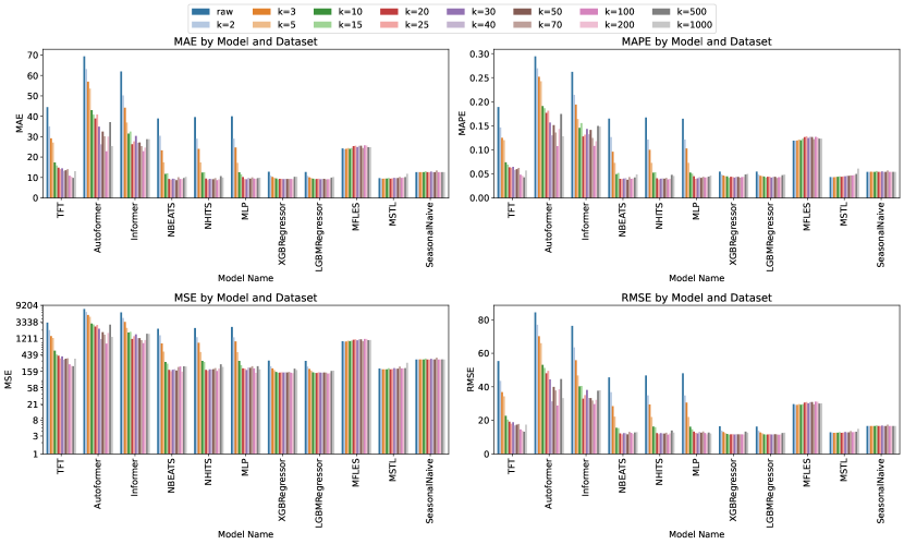
The evaluation of various forecasting methods is classified into four distinct groups: Baseline, Statistical, Machine Learning, and Neural Networks. These models are trained at varying levels of microaggregation, represented by . Their performance is evaluated using multiple metrics, aiming to offer a comprehensive analysis of how these techniques function across different data aggregation levels. The results obtained we display in \autoreffig:results.
III-A Comparison Across Categories
The baseline approach, represented by Seasonal Naive, overall exhibits constant metrics at all levels of microaggregation. This indicates that although simple and computationally inexpensive, the baseline approach can forecast accurately and is a valid baseline for the rest of the models.
Statistical approaches, including MSTL and MFLES, displayed mixed performance over the baseline. Specially, MSTL shows relatively stable performance across different levels. In contrast, MFLES has more variability in terms of performance, being worse than the baseline across all levels. This indicates that while MSTL can maintain consistent accuracy despite increasing anonymization, MFLES is more sensitive to these changes.
ML approaches, such as XGBRegressor and LGBMRegressor, demonstrate competitive performance, often achieving lower error metrics compared to statistical methods. For instance LGBMRegressor with obtained the best overall MSE and RMSE with values of 138.38 and 11.43 respectively.
These approaches leverage ensemble techniques and gradient boosting, which enhance their ability to model complex relationships within the data. Furthermore, ML approaches handle changes in relatively well, maintaining competitive and constant performance across different levels.
Within the NN approaches, two subfamilies perform differently. On the one hand the MLP-base models namely: NHITS, MLP, NBEATS displays a good performance in general. Particularly performant for NBEATS with for which it obtained the overall best MAE, MAPE and SMAPE of 8.65, 0.037 and 0.018 respectively. On the other hand the transformer-based models notably: Autoformer, Informer and TFT achieve the overall worst performance across most metrics. In particular the Autoformer when trained on raw data is the overall worst-performing model of the evaluation with 69.39, 0.29, 7286.95, 84.43 and 0.16 of MAE, MAPE, MSE, RMSE and SMAPE respectively. These results suggest a severe overfitting case.
In general for both subfamilies we can oversee a similar pattern in which the model performance increases as the increases. It is noteworthy to mention that under high anonymization regimes the models found the best performing stage. Particularly the DL models find their optimal , similarly the ML models find their minima at slightly less restrictive anonymity . On the contrary Transformers find their best performing regime at ,
NBEATS is an exemplary model with an accentuated performance increase as k increases. NBEATS performs suboptimal on raw data but has a considerable improvement on high anonymization levels. For instance, the MAE of NBEATS ranges from 38.92 kw/hh using raw data to 8.65 kw/hh when trained with () when it finds their performance maxima.
III-B Impact of Microaggregation Levels
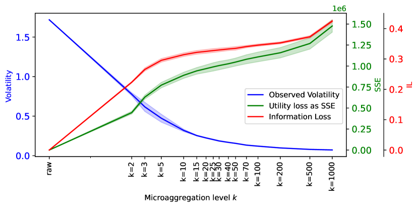
As the microaggregation level increases; changes in the dynamics of the dataset and thus the way models learn. To evaluate the impact of microaggregation on the datasets, we used the Sum of Squared Errors (SSE) [24] (see Eq. (3)) and the Information Loss (IL) [25] (see Eq. (4)) to measure the information loss and finally to analyze how the dataset’s volatility changes as we increase in anonymization level we used Eq. (5) In the previous equations, represents the anonymized dataset, while corresponds to the original dataset. Here, denotes the number of elements to be anonymized, and indicates the number of observations per element.
| (3) |
| (4) |
| (5) |
To ensure a more robust utility-volatility analysis, we generated 10 distinct microaggregated datasets with 1000 households each from our original set in II-A. The bold line represents the average, and the shaded area represents the standard deviation of the runs. The figure illustrates that there are no substantial variations among the datasets analyzed.
In Figure 3, the volatility in the dataset decreases as increases. To illustrate this loss, we fitted an exponential decay function (see Eq. (6)), which fits with an value of 0.86.
| (6) |
The quasi-exponential decay in variability within the time series may explain why more complex and larger models tend to overfit the noise, whereas simpler, more trend-focused models perform better in highly volatile scenarios. Overall, as increases, the performance of the models also improves. A similar pattern is observed in clustering because the data points within each cluster become more homogeneous. This reduction in within-cluster variability makes it easier for forecasting models to identify patterns and forecast accurately [26].
Furthermore, the SSE quantifies the total deviation of data points from their cluster centroids after microaggregation and IL measures the average difference between the actual values and their approximations, adjusted by the variability of each feature in the data.
As increases, the number of data points in each group also increases, leading to a reduction in the group volatility. This is because larger clusters tend to average out more of the individual variations, resulting in more homogeneous centroids. This information is also visible as the decay in variability indicates that the clusters are becoming more uniform, which simplifies the structure of the data.
Consequently, simpler models that focus on broader trends rather than intricate details perform better, as they are less likely to overfit the noise present in the data. Overall: models, IL and SSE and volatility stabilize at around , as indicated by the red dotted line. This statement poses profound implications for both researchers and practitioners. Our experiments display that after , adding anonymization to the model is basically a free lunch. Before this point, anonymization is pricey since it produces a quasi-exponential increase in information loss.
IV Discussion
The findings of this study underscore the viability of using microaggregation as an effective anonymization technique for electric load profiles without significantly compromising the accuracy of forecasting models by evaluating them at an aggregated level. This is particularly relevant in the context of the GDPR, which mandates stringent measures to protect personal data. By demonstrating that microaggregated data can maintain high levels of utility, this research addresses a critical challenge in the energy sector: balancing privacy with data usability.
Our findings indicate that, for instance, DSOs or energy suppliers could provide access to their data set by anonymizing their data to comply with regulations. Yet, at the same time, energy suppliers could use such an approach at an aggregated level because it provides clustering benefits, effectively killing two birds with one stone. The reduced volatility within groups enhances model learning by minimizing noise, which improves model fit as group size increases. Additionally, our results suggest a plateau of information loss between to , where the increase in SSE and IL is not as linear as the rise in protection levels, suggesting an optimal range for balancing privacy and data utility.
However, this study is not without limitations. The public dataset used, while extensive, is limited to a specific geographic region, time frame, and year and might not capture current trends (decentralization and electrification of assets). Additionally, while microaggregation has potential, further exploration of other anonymization techniques such as [11] and their impact on forecasting accuracy is needed over larger periods to seek consistency. Lastly, this paper evaluates the forecasting performance at an aggregated level; further research could evaluate to what extent this modelization could be applied to household-level forecasting.
V Conclusion
In conclusion, this study suggests that microaggregation is a viable technique for anonymizing electric load profiles, effectively balancing the need for privacy with the utility of the data. The minimal impact on forecasting accuracy observed across various models, in the case of aggregated level data, underscores the potential for integrating such anonymization methods into the energy sector. Such a technique could help unblock the scarcity and data complexity acquisition of smart meter data for research institutions, universities, or third-party companies while still complying with current European regulations and focusing on maintaining consumer privacy.
Declaration of Generative AI and AI-assisted technologies in the writing process
References
- [1] The European Commission, “Directive 2009/72/ec of the european parliament and of the council of 13 july 2009 concerning common rules for the internal market in electricity and repealing directive 003/54/ec,” Official Journal of the Europan Union, vol. L 211/55, 2009.
- [2] V. C. Gungor, D. Sahin, T. Kocak, S. Ergut, C. Buccella, C. Cecati, and G. P. Hancke, “Smart grid technologies: Communication technologies and standards,” IEEE Transactions on Industrial Informatics, vol. 7, no. 4, pp. 529–539, 2011.
- [3] F. Petropoulos, D. Apiletti, V. Assimakopoulos, M. Z. Babai, D. K. Barrow, S. B. Taieb, C. Bergmeir, R. J. Bessa, J. Bijak, J. E. Boylan, et al., “Forecasting: theory and practice,” International Journal of Forecasting, vol. 38, no. 3, pp. 705–871, 2022.
- [4] J. Zheng, D. W. Gao, and L. Lin, “Smart meters in smart grid: An overview,” in 2013 IEEE Green Technologies Conference (GreenTech), pp. 57–64, 2013.
- [5] B. Wolford, “What is GDPR, the EU’s new data protection law?,” 2018. Accesed on: 20/06/2024.
- [6] C. Efthymiou and G. Kalogridis, “Smart grid privacy via anonymization of smart metering data,” in 2010 First IEEE International Conference on Smart Grid Communications, pp. 238–243, IEEE, 2010.
- [7] J. Domingo-Ferrer and V. Torra, “Ordinal, continuous and heterogeneous k-anonymity through microaggregation,” Data Mining and Knowledge Discovery, vol. 11, pp. 195–212, 2005.
- [8] J. Wang, F. Gao, Y. Zhou, Q. Guo, C.-W. Tan, J. Song, and Y. Wang, “Data sharing in energy systems,” Advances in Applied Energy, vol. 10, p. 100132, 2023.
- [9] G. Strbac, S. Tindemans, M. Woolf, M. Bilton, R. Carmichael, and J. R. Schofield, “Low Carbon London Project: Data from the Dynamic Time-of-Use Electricity Pricing Trial, 2013,” 2024.
- [10] L. Sweeney, “k-anonymity: A model for protecting privacy,” International journal of uncertainty, fuzziness and knowledge-based systems, vol. 10, no. 05, pp. 557–570, 2002.
- [11] K. S. Adewole and V. Torra, “Dftmicroagg: a dual-level anonymization algorithm for smart grid data,” International Journal of Information Security, vol. 21, no. 6, pp. 1299–1321, 2022.
- [12] K. Bandara, R. J. Hyndman, and C. Bergmeir, “Mstl: A seasonal-trend decomposition algorithm for time series with multiple seasonal patterns,” arXiv preprint arXiv:2107.13462, 2021.
- [13] B. Tyler, “MFLES,” 2024.
- [14] T. Chen and C. Guestrin, “Xgboost: A scalable tree boosting system,” arXiv preprint arXiv:1603.02754, 2016.
- [15] G. Ke, Q. Meng, T. Finley, T. Wang, W. Chen, W. Ma, Q. Ye, and T.-Y. Liu, “Lightgbm: A highly efficient gradient boosting decision tree,” Advances in Neural Information Processing Systems, 2017.
- [16] B. N. Oreshkin, D. Carpov, N. Chapados, and Y. Bengio, “N-beats: Neural basis expansion analysis for interpretable time series forecasting,” arXiv preprint arXiv:1905.10437, 2019.
- [17] C. Challu, G. Marcjasz, P. Montero-Manso, T. S. Talagala, R. J. Hyndman, and R. J. Bessa, “N-hits: Neural hierarchical interpolation for time series forecasting,” arXiv preprint arXiv:2201.12886, 2022.
- [18] H. Wu, J. Xu, J. Wang, and M. Long, “Autoformer: Decomposition transformers with auto-correlation for long-term series forecasting,” arXiv preprint arXiv:2106.13008, 2021.
- [19] H. Zhou, S. Zhang, J. Peng, S. Zhang, J. Li, H. Xiong, and W. Zhang, “Informer: Beyond efficient transformer for long sequence time-series forecasting,” arXiv preprint arXiv:2012.07436, 2020.
- [20] B. Lim, S. O. Arik, N. Loeff, and T. Pfister, “Temporal fusion transformers for interpretable multi-horizon time series forecasting,” arXiv preprint arXiv:1912.09363, 2019.
- [21] S. Varrette, P. Bouvry, H. Cartiaux, and F. Georgatos, “Management of an academic hpc cluster: The ul experience,” in Proc. of the 2014 Intl. Conf. on High Performance Computing & Simulation (HPCS 2014), (Bologna, Italy), pp. 959–967, IEEE, July 2014.
- [22] K. G. Olivares, C. Challú, F. Garza, M. M. Canseco, and A. Dubrawski, “NeuralForecast: User friendly state-of-the-art neural forecasting models..” PyCon Salt Lake City, Utah, US 2022, 2022.
- [23] F. Garza, M. M. Canseco, and K. G. O. Cristian Challú, “StatsForecast: Lightning fast forecasting with statistical and econometric models.” PyCon Salt Lake City, Utah, US 2022, 2022.
- [24] J. Domingo-Ferrer and Y. Saygin, Privacy in statistical databases, vol. 5262. Springer, 2008.
- [25] W. E. Yancey, W. E. Winkler, and R. H. Creecy, Disclosure risk assessment in perturbative microdata protection. Springer, 2002.
- [26] J. D. Fernandez, S. Potenciano Menci, and I. Pavic, “Towards a peer-to-peer residential short-term load forecasting with federated learning,” in 2023 IEEE Belgrade PowerTech, pp. 1–6, 2023.
- [27] “DeepL.” \urlhttps://www.deepl.com/write.
- [28] “ChatGPT.” \urlhttps://chatgpt.com/.