Optimizing Supply Chain Networks with the Power of Graph Neural Networks

Abstract

Graph Neural Networks (GNNs) have emerged as transformative tools for modeling complex relational data, offering unprecedented capabilities in tasks like forecasting and optimization. This study investigates the application of GNNs to demand forecasting within supply chain networks using the SupplyGraph dataset, a benchmark for graph-based supply chain analysis. By leveraging advanced GNN methodologies, we enhance the accuracy of forecasting models, uncover latent dependencies, and address temporal complexities inherent in supply chain operations. Comparative analyses demonstrate that GNN-based models significantly outperform traditional approaches, including Multilayer Perceptrons (MLPs) and Graph Convolutional Networks (GCNs), particularly in single-node demand forecasting tasks. The integration of graph representation learning with temporal data highlights GNNs’ potential to revolutionize predictive capabilities for inventory management, production scheduling, and logistics optimization. This work underscores the pivotal role of forecasting in supply chain management and provides a robust framework for advancing research and applications in this domain.

Keywords Demand forecasting  $\cdot$ Production Planning  $\cdot$ Single node prediction  $\cdot$ Graph Neural Networks (GNNs)  $\cdot$ SupplyGraph Dataset

1 Introduction

Supply chain networks are highly intricate systems that coordinate interactions among products, manufacturing facilities, storage locations, and distribution centers. These interactions are governed by supply and demand dynamics, making the networks naturally suited for graph-based representations. Graph Neural Networks (GNNs) have emerged as powerful tools for analyzing such relational data structures, enabling insights that are challenging to achieve with traditional methods [1, 2, 3]. Their success in diverse domains—including social network analysis [4], transportation systems [5], weather prediction [6], and knowledge graph reasoning [7]—demonstrates their capacity to model complex dependencies and dynamic interactions.

Despite the significant promise of GNNs, their application in supply chain management has been relatively limited, largely due to the absence of publicly available datasets that capture the multifaceted nature of supply chain operations. Traditional machine learning models, including Multilayer Perceptrons (MLPs) and Long Short-Term Memory networks (LSTMs), have been employed for tasks like demand forecasting and production scheduling, but they often fail to fully exploit the relational structures within supply chain networks [8, 9]. Recent advances in graph representation learning suggest that GNNs can address these limitations by uncovering hidden dependencies and enabling more accurate predictions [10].

The introduction of the SupplyGraph dataset [11] marks a turning point in the application of GNNs to supply chain analytics. Derived from real-world operations at a leading Fast-Moving Consumer Goods (FMCG) company in Bangladesh, this dataset models supply chain elements as nodes and their interdependencies as edges, incorporating temporal features such as production volumes, sales orders, delivery metrics, and factory issues. By integrating temporal and relational data, the SupplyGraph dataset facilitates the exploration of tasks such as demand forecasting, anomaly detection, and resource optimization.

Leveraging the inherent graph structure of supply chain networks, GNNs have the potential to transform supply chain management. By modeling both local and global dependencies, GNNs can uncover patterns that are not apparent through traditional machine learning approaches [2, 10, 12]. This capability is particularly critical for demand forecasting, where accurate predictions are essential for inventory management, production scheduling, and operational efficiency [13, 14].

In this study, we aim to address the current limitations in applying GNNs to supply chain management by providing a comprehensive analysis of the SupplyGraph dataset. Specifically, we focus on these two goals: 1)Define key downstream tasks relevant to supply chain management, such as demand forecasting. 2)Establish baseline performance metrics using GNN-based models to evaluate their effectiveness.

While the SupplyGraph dataset offers a robust foundation for graph-based supply chain analytics, its utility has been hindered by the lack of standardized downstream tasks and benchmarks. This work bridges that gap by introducing a framework for actionable applications and evaluating the performance of GNN-based models on critical supply chain tasks. By doing so, we demonstrate the practical and theoretical value of GNNs in optimizing supply chain networks and fostering advancements in predictive modeling for complex, real-world systems.

2 Related Work

The intersection of supply chain management and machine learning has seen significant advancements, particularly in optimizing production planning and demand forecasting. Traditional approaches frequently employ methods such as Artificial Neural Networks (ANNs) [15], Convolutional Neural Networks (CNNs) [16], and Long Short-Term Memory (LSTM) models [8] to enhance forecasting accuracy, inventory management, and production scheduling. While these methods have shown promise, they often fall short in fully exploiting the relational structures inherent in supply chain networks [8, 9].

Graph Neural Networks (GNNs), a relatively recent innovation, have demonstrated exceptional capabilities in handling graph-structured data across various domains. In social network analysis, GNNs have been employed to model user interactions and improve recommendation systems [4]. In the field of drug discovery, GNNs have accelerated the prediction of molecular properties and drug-protein interactions [17]. Additionally, in biomedical signal processing, GNNs have advanced brain-computer interface technologies through multimodal data analysis [18, 19]. These successes underscore their potential to uncover complex dependencies and dynamic interactions in supply chain networks.

Despite their promise, GNNs have been underutilized in supply chain analytics, primarily due to the lack of publicly available, real-world datasets. This gap has hindered benchmarking and innovation in this field. Recent studies have explored GNN applications in tasks like link prediction and hidden dependency analysis, which are critical for mitigating risks and improving decision-making in supply chain management [20, 21].

The introduction of the SupplyGraph dataset [11] addresses this limitation by providing a comprehensive benchmark tailored for GNN applications in supply chain analytics. This dataset encapsulates the complexities of supply chain operations, including temporal features such as production volumes, sales orders, and delivery metrics. By integrating graph representation learning with temporal data, the SupplyGraph dataset facilitates diverse tasks, such as demand forecasting, anomaly detection, and resource optimization.

Recent advancements in graph representation learning methodologies, such as Graph Convolutional Networks (GCNs) [2], Graph Attention Networks (GATs) [22], and Graph Isomorphism Networks (GINs) [23], further enhance the applicability of GNNs in supply chain management. These approaches enable the modeling of intricate relationships and dependencies, offering transformative potential for predictive tasks like demand forecasting and production planning.

This work builds on these advancements, demonstrating the practical and theoretical value of GNNs in optimizing supply chain networks. By bridging the gap between theoretical graph methodologies and practical applications, it fosters new opportunities for innovation in this critical domain.

3 Tasks Definition

The primary contributions of this paper are the definition of downstream tasks and the release of related open-source code. In this section, we introduce the tasks.

3.1 The Structure of the SupplyGraph Dataset

The SupplyGraph dataset was developed to address the lack of real-world benchmark datasets for applying Graph Neural Networks (GNNs) in supply chain research. Derived from the central database of a leading Fast-Moving Consumer Goods (FMCG) company, this dataset encapsulates the intricate complexities of supply chain networks by incorporating a rich array of nodes, edges, and temporal features. These elements capture the dynamic and interconnected nature of modern supply chain operations.

In the SupplyGraph dataset, nodes represent distinct products, which are categorized into product groups, sub-groups, production plants, and storage locations. Each node is further enriched with temporal features, such as production levels, sales orders, delivery data, and factory issues, providing a temporal dimension for in-depth supply chain analysis. Edges in the dataset define relationships between nodes, including shared production facilities, storage dependencies, and raw material requirements, effectively modeling the intricate dependencies that shape supply chain operations. Multiple edge types ensure a comprehensive representation of these relationships.

Temporal features form a crucial aspect of the dataset, spanning 221 time points, which allows researchers to explore temporal dynamics in supply chain networks. These dynamics include production quantities, sales orders, deliveries, and factory issues, measured in both units and metric tons. The dataset supports various graph formulations, ranging from homogeneous graphs with uniform node and edge types to heterogeneous graphs reflecting the diverse interactions in complex supply chains. Notably, only a homogeneous graph version is provided in the folder Raw Dataset/Homogenoeus, and constructing heterogeneous graphs requires manual structuring.

The dataset comprises 41 distinct products as nodes and 684 unique edges representing various relationships. Nodes are grouped into five major product categories, 19 sub-groups, 25 production plants, and 13 storage locations, offering a detailed and multi-dimensional view of supply chain operations. With its comprehensive structure and rich temporal features, the SupplyGraph dataset serves as a robust foundation for advancing research in supply chain analytics. It enables critical tasks such as demand forecasting, production planning, risk assessment, and anomaly detection. By bridging the gap between theoretical advancements in GNN methodologies and practical applications in supply chain management, the dataset fosters innovative opportunities in this vital domain.

3.2 Demand Forecasting Based on Single Node

The single-node demand forecasting task in the SupplyGraph dataset focuses on predicting the future demand for an individual node—such as a factory, storage location, or distribution center—using its historical data and contextual information.1

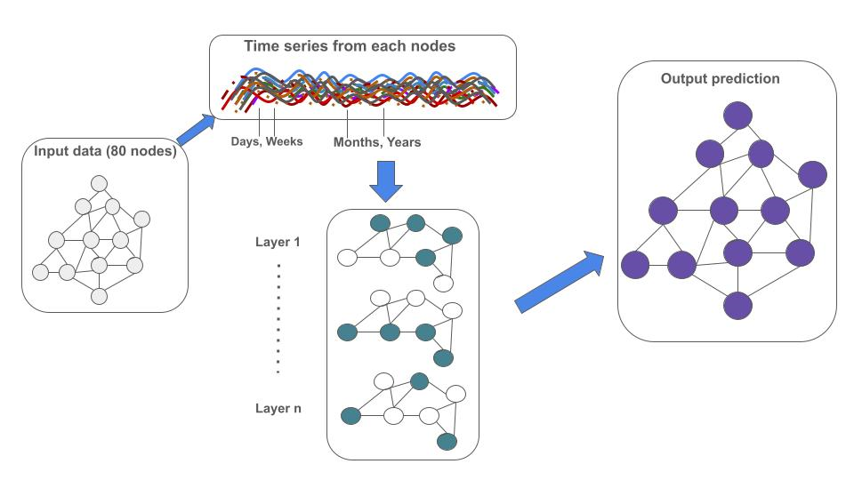
Figure 1: A conceptual workflow for GNNs demand forecasting for single node.

This task is a critical component of supply chain management, as it facilitates better inventory planning, production scheduling, and overall operational efficiency. Nodes in the dataset are characterized by temporal features (e.g., sales orders, production outputs) and static attributes (e.g., node type or group). By leveraging historical demand patterns, seasonal trends, and short-term fluctuations, this task aims to provide accurate demand forecasts over both short-term horizons (e.g., the next week) and long-term horizons (e.g., the next quarter).

This task utilizes data from files such as Sales Order.csv and Production.csv to model demand dynamics for specific nodes, for example, SOS008L02P. The input data typically includes recent time-series observations, while the outputs predict demand for future time intervals. Techniques such as sliding window methods are employed to extract relevant historical features, which are then fed into machine learning models or statistical algorithms. As a pivotal component of supply chain analytics, this forecasting task enhances the performance of individual nodes and contributes to the overall efficiency and resilience of the supply chain system.

4 Methodology

4.1 Multilayer Perceptron (MLP)

A Multilayer Perceptron (MLP) is a type of artificial neural network designed as a feedforward network, meaning that information flows in one direction—from the input layer, through one or more hidden layers, and finally to the output layer. Each layer is fully connected, with every neuron (node) in one layer connected to every neuron in the next. The MLP is a powerful model capable of learning and representing complex non-linear relationships in data through its multi-layered architecture and non-linear activation functions.

Key Components of an MLP

1. Input Layer: This layer receives the input features $\mathbf{x}\in\mathbb{R}^{d}$, where $d$ represents the dimensionality of the input data.

2. Hidden Layers: Each hidden layer applies a linear transformation followed by a non-linear activation function, enabling the network to model complex patterns. The transformation at each layer $l$ can be expressed as:

   $$\mathbf{h}^{(l)}=\sigma(\mathbf{W}^{(l)}\mathbf{h}^{(l-1)}+\mathbf{b}^{(l)}),\quad l=1,2,\dots,L,$$

   where:

   • $\mathbf{h}^{(l)}$ is the output of the $l$-th layer.

   • $\mathbf{W}^{(l)}\in\mathbb{R}^{m_{l}\times m_{l-1}}$ are the weights.

   • $\mathbf{b}^{(l)}\in\mathbb{R}^{m_{l}}$ are the biases.

   • $\sigma(\cdot)$ is the activation function (e.g., ReLU, sigmoid, or tanh).

3. Output Layer: This layer produces the network’s final output, with a task-specific activation function such as softmax for classification or linear for regression tasks.

Training and Applications

MLPs are trained using the backpropagation algorithm [24], which computes gradients of a loss function (e.g., cross-entropy for classification or mean squared error for regression) with respect to weights and biases. These gradients are used to iteratively update the model parameters via optimization methods like stochastic gradient descent (SGD) or its variants (e.g., Adam). MLPs have been widely employed across various domains due to their versatility: 1) Classification: Tasks such as image recognition, text classification, and sentiment analysis [16]. 2)Regression: Applications in predictive analytics, time series forecasting, and financial modeling. 3)Feature Extraction*: Representation learning for dimensionality reduction and clustering.

Advantages and Limitations

MLPs are universal approximators, capable of approximating any continuous function given sufficient hidden units and training data [25].Their flexibility allows them to be applied to a wide range of problems. However, MLPs often require significant computational resources and careful hyperparameter tuning. They are prone to overfitting, especially when the dataset is small or imbalanced.Compared to specialized architectures like Convolutional Neural Networks (CNNs) or Transformers, MLPs may struggle with structured or sequential data. Overall, the MLP forms the foundational building block of deep learning architectures and has inspired the development of more advanced neural networks. Despite its simplicity, it remains a crucial tool in the field of machine learning.

4.2 Graph Neural Networks (GNN)

Graph Neural Networks (GNNs) are a class of deep learning models designed to operate on graph-structured data. A graph, defined as $G=(V,E)$, consists of a set of nodes (or vertices) $V$ and edges $E$ that represent relationships between the nodes. In many applications, graphs are accompanied by features on nodes ($\mathbf{X}\in\mathbb{R}^{|V|\times d}$) and possibly on edges ($\mathbf{E}$). GNNs leverage this structure to capture the inherent relationships and dependencies between entities in the graph, making them powerful tools for analyzing relational data.

Mathematical Framework

The core operation of a GNN involves the iterative exchange and aggregation of information (messages) between nodes over their neighborhoods. This process is typically composed of the following steps at each layer $l$:

1. **Message Passing**: Information from neighboring nodes is aggregated to form a message for a target node:

$$\mathbf{m}_{v}^{(l)}=\text{AGGREGATE}(\{\mathbf{h}_{u}^{(l-1)}\mid u\in\mathcal{N}(v)\}),$$

where $\mathbf{h}_{u}^{(l-1)}$ represents the embedding of node $u$ from the previous layer, and $\mathcal{N}(v)$ is the set of neighbors of node $v$.

2. **Node Update**: The node’s representation is updated based on the aggregated message and its current state:

$$\mathbf{h}_{v}^{(l)}=\text{UPDATE}(\mathbf{h}_{v}^{(l-1)},\mathbf{m}_{v}^{(l)}).$$

3. **Readout (Optional)**: For tasks like graph classification, a global representation is computed by aggregating node embeddings:

$$\mathbf{h}_{G}=\text{READOUT}(\{\mathbf{h}_{v}^{(L)}\mid v\in V\}),$$

where $L$ is the number of layers in the GNN.

Key Features and Variants

Graph Neural Networks (GNNs) are highly expressive models that generalize convolutional operations to graph-structured data, allowing them to effectively learn from both node attributes and the underlying structural relationships. Several notable variants of GNNs have been developed to enhance their capabilities. Graph Convolutional Networks (GCNs) [2] extend traditional convolutional operations to graphs, enabling the aggregation of neighborhood information. Graph Attention Networks (GATs) [22] introduce attention mechanisms that assign different weights to neighbors, prioritizing more influential connections during learning. Graph Isomorphism Networks (GINs) [23] are designed to achieve higher expressive power by leveraging techniques inspired by the Weisfeiler-Lehman graph isomorphism test, making them capable of distinguishing more complex graph structures. Together, these variants demonstrate the versatility and adaptability of GNNs across a wide range of graph-based tasks.

Applications

Graph Neural Networks (GNNs) have found extensive applications across a wide range of fields due to their ability to process and analyze graph-structured data. In social networks, GNNs are utilized for tasks such as community detection, user recommendation, and social influence prediction. In the domain of molecular and biological graphs, they play a crucial role in drug discovery, protein interaction prediction, and genomics [26]. Knowledge graphs benefit from GNNs in reasoning, entity classification, and relation prediction tasks [7]. Similarly, in supply chain and transportation networks, GNNs are employed for dependency analysis and route optimization. Furthermore, they are increasingly used in natural language processing tasks, including semantic parsing, machine translation, and representing language structures as graphs, demonstrating their versatility and impact across disciplines.

Advantages and Limitations

Graph Neural Networks (GNNs) offer several advantages that make them highly suitable for analyzing complex, relational data. They can effectively model data with arbitrary structures, providing flexibility across various graph types, such as weighted, directed, and dynamic graphs. Additionally, GNNs are scalable to large graphs through techniques like sampling and exploiting graph sparsity, enabling their application to real-world problems with extensive data. However, GNNs also have notable limitations. They can suffer from over-smoothing as the network depth increases, where node representations become indistinguishable [27]. Furthermore, GNNs are computationally intensive, particularly for very large graphs, posing challenges for resource-constrained environments. Finally, their expressiveness is somewhat limited compared to higher-order models, such as hypergraph networks, which can capture more complex relationships and interactions.

4.3 Graph Convolutional Networks (GCNs)

Graph Convolutional Networks (GCNs) are a foundational type of Graph Neural Network (GNN) that extend the concept of convolution from Euclidean data (e.g., images) to graph-structured data. Introduced by Kipf and Welling [2], GCNs are specifically designed to learn node embeddings by aggregating and transforming information from a node’s local neighborhood, leveraging both the graph structure and node attributes.

Mathematical Definition

A graph is defined as $G=(V,E)$, where $V$ is the set of nodes and $E$ is the set of edges. For a graph with $|V|$ nodes, let $\mathbf{A}\in\mathbb{R}^{|V|\times|V|}$ denote the adjacency matrix, and let $\mathbf{X}\in\mathbb{R}^{|V|\times d}$ represent the node feature matrix, where each row corresponds to the $d$-dimensional feature vector of a node. A single GCN layer updates node representations as follows:

$$\mathbf{H}^{(l)}=\sigma\left(\hat{\mathbf{A}}\mathbf{H}^{(l-1)}\mathbf{W}^{(l)}\right),$$

where:

• $\mathbf{H}^{(l)}\in\mathbb{R}^{|V|\times d_{l}}$ is the matrix of node embeddings at layer $l$.

• $\mathbf{H}^{(0)}=\mathbf{X}$ is the input feature matrix.

• $\hat{\mathbf{A}}=\tilde{\mathbf{D}}^{-1/2}\tilde{\mathbf{A}}\tilde{\mathbf{D}}^{-1/2}$ is the symmetric normalized adjacency matrix.

• $\tilde{\mathbf{A}}=\mathbf{A}+\mathbf{I}$ adds self-loops to the adjacency matrix.

• $\tilde{\mathbf{D}}$ is the degree matrix of $\tilde{\mathbf{A}}$.

• $\mathbf{W}^{(l)}\in\mathbb{R}^{d_{l-1}\times d_{l}}$ is the learnable weight matrix at layer $l$.

• $\sigma(\cdot)$ is a non-linear activation function, such as ReLU or tanh.

By stacking multiple GCN layers, the model can capture higher-order neighborhood information, enabling it to aggregate features from nodes multiple hops away.

Key Features of GCNs

1. Aggregation and Transformation*: Each layer combines information from a node’s neighbors and applies learnable transformations, effectively propagating and transforming information across the graph.

2. Normalization: The use of $\hat{\mathbf{A}}$ ensures that feature aggregation is normalized, preventing issues like exploding or vanishing gradients.

3. End-to-End Learning: GCNs are trained in an end-to-end manner, often using supervised learning objectives.

Variants and applications of GCNs

Several notable extensions of Graph Convolutional Networks (GCNs) have been developed to address specific challenges and enhance their capabilities. FastGCN [28] improves the efficiency of GCNs by employing a node sampling strategy, significantly reducing computational costs when working with large-scale graphs. GraphSAGE [29] extends GCNs to enable inductive learning, allowing the model to generalize to unseen nodes and dynamic graph structures, making it suitable for large and evolving datasets. Graph Attention Networks (GATs) [22] introduce attention mechanisms to assign different weights to neighboring nodes, enabling the model to focus on the most relevant connections during aggregation. These advancements demonstrate the adaptability of GCNs and their evolving role in addressing scalability, flexibility, and expressiveness in graph-based learning.

Graph Convolutional Networks (GCNs) are widely applied across various domains due to their ability to effectively analyze graph-structured data. In node classification, GCNs predict labels for nodes in a graph, often in semi-supervised or unsupervised settings, with common applications in citation networks and social graphs. For link prediction, GCNs estimate the likelihood of edges between nodes, which is particularly useful in recommendation systems and knowledge graph completion. They are also extensively used for graph classification, where entire graphs are assigned labels, a task frequently encountered in bioinformatics, such as molecule classification. Additionally, GCNs play a significant role in spatial data analysis, powering applications in transportation networks, climate modeling, and geographic information systems, showcasing their versatility in addressing complex, structured data across multiple fields.

Advantages and Limitations

Graph Convolutional Networks (GCNs) offer several advantages, making them a foundational tool in graph-based machine learning. They effectively capture both structural and feature-based information, enabling a comprehensive understanding of graph data. GCNs are scalable to moderately large graphs, thanks to their reliance on sparse matrix operations, and their simplicity and versatility have established them as the basis for many advanced Graph Neural Network (GNN) models. However, GCNs have notable limitations. As the number of layers increases, they may suffer from over-smoothing, where node representations become indistinguishable [27]. Additionally, scalability becomes a challenge for very large graphs due to growing computational costs. Finally, GCNs have limited expressiveness in distinguishing complex graph structures compared to more advanced models like Graph Isomorphism Networks (GINs) [23], highlighting areas for further improvement and specialization.

5 Experiments

5.1 Data Preprocessing

Data preprocessing involves several essential steps to ensure clean, consistent, and reliable data for analysis. First, edge and node data are processed to remove duplicate rows and entries with insufficient data points, ensuring that all datasets contain unique and valid observations. Temporal data is refined by eliminating rows with missing values and normalizing numerical features using the z-score method. This normalization ensures consistent scaling across features, improving compatibility for subsequent analysis. Lastly, low-quality nodes—those with a high proportion of zero values in their temporal features—are identified and excluded. These preprocessing measures collectively enhance data integrity, usability, and suitability for advanced modeling tasks.

5.2 Performance Metrics

Evaluation metrics are critical for assessing the performance of predictive models. Two commonly used metrics in this study are Mean Absolute Error (MAE) and Mean Squared Error (MSE), each providing unique insights into model accuracy.

5.2.1 Mean Absolute Error (MAE)

MAE measures the average magnitude of errors in a set of predictions, regardless of their direction. It is defined as:

$$\text{MAE}=\frac{1}{n}\sum_{i=1}^{n}\lvert y_{i}-\hat{y}_{i}\rvert$$

where $y_{i}$ represents the actual value, $\hat{y}_{i}$ the predicted value, and $n$ the number of data points. By focusing on absolute differences, MAE provides an interpretable metric in the same units as the target variable. This makes it particularly useful when large deviations should not be disproportionately penalized.

5.2.2 Mean Squared Error (MSE)

MSE evaluates the average of the squared differences between predicted and actual values, expressed as:

$$\text{MSE}=\frac{1}{n}\sum_{i=1}^{n}(y_{i}-\hat{y}_{i})^{2}$$

Unlike MAE, MSE amplifies the effect of larger errors due to squaring, making it more sensitive to outliers. This sensitivity is advantageous in scenarios where large prediction errors have significant implications. However, its interpretation is less intuitive, as the resulting values are in squared units of the target variable.

Both MAE and MSE are indispensable tools, with their applicability depending on the specific requirements of the task. MAE is robust to outliers, offering a balanced perspective on overall accuracy, while MSE emphasizes substantial errors, favoring models with fewer extreme deviations.

In this study, MAE and MSE are employed to evaluate the predictive performance of MLP, GNN, and GCN models, providing complementary insights into their strengths and weaknesses.

5.3 Implementation Details

This study implemented and trained multiple models, including a Multi-Layer Perceptron (MLP), Graph Neural Network (GNN), and Graph Convolutional Network (GCN). Each model was trained for 50 epochs to ensure sufficient learning while minimizing the risk of overfitting. The dataset was divided into three subsets with a 7:2:1 ratio, corresponding to training, validation, and testing sets. This split ensures adequate data for model training while reserving sufficient samples for reliable validation and testing.

The models were optimized using the Adam optimizer with a learning rate of 0.001. This choice of hyperparameters was made to promote stable and efficient convergence during the training process. Together, these implementation details provide a robust framework for evaluating and comparing the performance of the models across the tasks.

5.4 Results

5.4.1 Demand Forecasting based on Single Node

This study employs a Graph Neural Network (GNN) model designed with fully connected layers to process a dataset consisting of $164$ nodes. By incorporating a temporal window of size window_size, the input data is expanded to $164\times\text{window\_size}$ nodes, enabling the model to effectively capture temporal dynamics. The GNN model uses an identity matrix as the adjacency matrix, assuming no explicit connections between nodes and focusing solely on self-loops. This simplification emphasizes node-specific transformations while maintaining computational efficiency.

Node features are reshaped into a tensor format suitable for matrix operations, with the adjacency matrix expanded across batches to allow independent processing of graph structures for each sample. The model aggregates information by performing batch-wise matrix multiplication between the adjacency matrix and node features. These transformed features are then flattened and passed through fully connected layers, each applying a linear transformation followed by ReLU activation. This architecture facilitates the extraction of complex, higher-order representations, even without explicit inter-node connections.

The GNN processes features for $164$ nodes within each temporal window, leveraging the adjacency matrix to perform localized self-looped transformations. While the use of an identity matrix restricts information flow to individual nodes, the multi-layer design compensates by enabling the model to capture intricate non-linear dependencies. This approach is particularly effective for datasets where temporal or spatial relationships are not explicitly defined but still contain valuable patterns.

Key Insights and Implications

• Temporal Dynamics and Feature Extraction: By incorporating a temporal window, the model captures sequential dependencies, enabling it to identify trends and patterns across time. This is particularly beneficial for time-series datasets where temporal relationships play a critical role in prediction accuracy.

• Scalability and Flexibility: The use of batch-wise operations and an identity matrix allows the model to scale efficiently to larger datasets with fixed node counts. Moreover, the architecture can be extended to datasets with explicit graph structures by replacing the identity matrix with a meaningful adjacency matrix, enhancing the model’s versatility.

• Performance on Complex Relationships: Despite the absence of explicit connections between nodes, the multi-layer architecture captures complex, non-linear relationships effectively. This demonstrates the model’s ability to uncover meaningful patterns in datasets where dependencies are not explicitly encoded.

• Suitability for Graph-Based Time-Series Analysis: The model’s design aligns well with applications involving graph-based time-series data, such as demand forecasting, anomaly detection, and resource optimization. The ability to handle both temporal and structural data makes it a robust choice for diverse supply chain analytics tasks.

Future Directions

The current implementation highlights the potential of a GNN model with self-looped transformations for capturing meaningful representations in datasets with limited explicit connections. Future work could explore:

• Incorporating learned or domain-specific adjacency matrices to model explicit inter-node relationships.

• Extending the model to dynamic graphs where node and edge connections evolve over time.

• Benchmarking the model against state-of-the-art approaches on more complex graph datasets to further validate its performance.

Product	Model	MSE	MAE
POP015K	MLP	60.3381	5
POP015K	GNN	72.2665	6
POP015K	GCN	0.0000	0
MAPA1K24P	MLP	62.0172	6
MAPA1K24P	GNN	73.2651	7
MAPA1K24P	GCN	0.0000	0
MAR02K12P	MLP	59.9826	5
MAR02K12P	GNN	208.1954	1
MAR02K12P	GCN	0.0286	0
MAP1K25P	MLP	111.0879	7
MAP1K25P	GNN	276.8117	1
MAP1K25P	GCN	1.0749	0
SOS002L09P	MLP	98.8177	7
SOS002L09P	GNN	339.8684	1
SOS002L09P	GCN	0.0192	0
SE200G24P	MLP	52.1664	5
SE200G24P	GNN	21.7223	4
SE200G24P	GCN	0.0137	0
POP500M24P	MLP	114.9090	8
POP500M24P	GNN	108.4203	8
POP500M24P	GCN	0.0575	0
SOS500M24P	MLP	116.6315	9
SOS500M24P	GNN	140.2561	1
SOS500M24P	GCN	0.0324	0
POV005L04P	MLP	175.5900	1
POV005L04P	GNN	262.6172	1
POV005L04P	GCN	0.0166	0
SOS008L02P	MLP	91.6898	6
SOS008L02P	GNN	64.5908	5
SOS008L02P	GCN	0.0166	0
MAC1K25P	MLP	72.9204	6
MAC1K25P	GNN	109.7107	8
MAC1K25P	GCN	0.0060	0
SOS003L04P	MLP	141.0485	9
SOS003L04P	GNN	53.9673	6
SOS003L04P	GCN	0.0258	0
SOS005L04P	MLP	30.0671	4
SOS005L04P	GNN	112.6256	8
SOS005L04P	GCN	0.0220	0
ATN01K24P	MLP	122.7641	8
ATN01K24P	GNN	105.7882	9
ATN01K24P	GCN	0.0976	0
EEA200G24P	MLP	66.7062	6
EEA200G24P	GNN	181.4845	1
EEA200G24P	GCN	0.0000	0

Table 1: Comparison of Task 1 part 1 result of Test MSE and MAE for different models on various products.

Product	Model	MSE	MAE
AT5X5K	MLP	208.1395	1
AT5X5K	GNN	270.6911	1
AT5X5K	GCN	0.0252	0
POP002L09P	MLP	25.3917	4
POP002L09P	GNN	172.5721	1
POP002L09P	GCN	0.0380	0
MASR025K	MLP	142.9998	9
MASR025K	GNN	208.9150	1
MASR025K	GCN	0.0568	0
ATWWP002K12P	MLP	141.4947	1
ATWWP002K12P	GNN	41.0776	5
ATWWP002K12P	GCN	0.0202	0
POP001L12P	MLP	380.7928	1
POP001L12P	GNN	52.2923	6
POP001L12P	GCN	0.0211	0
MAHS025K	MLP	99.6580	7
MAHS025K	GNN	63.5510	6
MAHS025K	GCN	0.0878	0
SE500G24P	MLP	91.6525	7
SE500G24P	GNN	28.8340	4
SE500G24P	GCN	0.0141	0
SOP001L12P	MLP	144.2692	8
SOP001L12P	GNN	109.6878	8
SOP001L12P	GCN	0.0145	0
SOS001L12P	MLP	139.4787	9
SOS001L12P	GNN	99.6211	8
SOS001L12P	GCN	0.0500	0
POPF01L12P	MLP	231.3161	1
POPF01L12P	GNN	161.3595	1
POPF01L12P	GCN	0.0168	0
ATWWP001K24P	MLP	158.3902	1
ATWWP001K24P	GNN	81.8863	7
ATWWP001K24P	GCN	0.0004	0
POV001L24P	MLP	39.7773	5
POV001L24P	GNN	43.6791	5
POV001L24P	GCN	0.0553	0
POV500M24P	MLP	98.7183	7
POV500M24P	GNN	131.4704	8
POV500M24P	GCN	0.0599	0
ATN02K12P	MLP	78.9037	7
ATN02K12P	GNN	28.1820	4
ATN02K12P	GCN	0.0490	0
SOS250M48P	MLP	23.7162	3
SOS250M48P	GNN	75.0150	6
SOS250M48P	GCN	0.0218	0
MAR01K24P	MLP	92.5119	7
MAR01K24P	GNN	199.0928	1
MAR01K24P	GCN	0.0354	0
POV002L09P	MLP	185.9516	1
POV002L09P	GNN	271.1639	1
POV002L09P	GCN	0.0152	0
POP005L04P	MLP	17.8096	3
POP005L04P	GNN	109.0347	8
POP005L04P	GCN	0.0078	0

Table 2: Comparison of Task1 part2 result of Test MSE and MAE for different models on various products.

6 Discussion and Conclusion

This study demonstrates the potential of Graph Neural Networks (GNNs) in addressing critical challenges in supply chain analytics, particularly in demand forecasting for individual nodes. By employing a model based on fully connected layers and leveraging temporal features, the GNN effectively captures meaningful patterns within time-series data, even in the absence of explicit inter-node connections. The identity matrix as the adjacency matrix simplifies computations while enabling the model to focus on self-looped transformations, which are crucial for extracting node-specific temporal insights. This approach provides a robust framework for handling datasets with fixed node counts and time-dependent characteristics.

The findings highlight the scalability and flexibility of the proposed GNN architecture. Its ability to adapt to diverse graph structures makes it suitable for a wide range of applications, including anomaly detection, resource optimization, and production planning. Despite the use of a simplified adjacency matrix, the model effectively learns non-linear relationships, demonstrating its capability to uncover hidden dependencies in complex supply chain systems. These results establish a strong foundation for exploring more advanced GNN methodologies tailored to supply chain management tasks.

Future work could focus on enhancing the model by incorporating domain-specific or learned adjacency matrices to capture explicit inter-node relationships and dependencies. Extending the approach to dynamic graphs, where nodes and edges evolve over time, could further improve the model’s applicability to real-world scenarios. Additionally, benchmarking the performance of this GNN architecture against state-of-the-art models on more complex datasets would provide deeper insights into its strengths and limitations. Such advancements have the potential to significantly contribute to the development of predictive tools for supply chain analytics and beyond.

References

- Scarselli et al. [2008] Franco Scarselli, Marco Gori, Ah Chung Tsoi, Markus Hagenbuchner, and Gabriele Monfardini. The graph neural network model. IEEE transactions on neural networks, 20(1):61–80, 2008.
- Kipf and Welling [2017] T. N. Kipf and M. Welling. Semi-supervised classification with graph convolutional networks. arXiv preprint arXiv:1609.02907, 2017.
- Velickovic et al. [2017] Petar Velickovic, Guillem Cucurull, Arantxa Casanova, Adriana Romero, Pietro Lio, and Yoshua Bengio. Graph attention networks. arXiv preprint arXiv:1710.10903, 2017.
- Guo and Wang [2020] Zhiwei Guo and Heng Wang. A deep graph neural network-based mechanism for social recommendations. IEEE Transactions on Industrial Informatics, 17(4):2776–2783, 2020.
- Li et al. [2018a] Yaguang Li, Rose Yu, Cyrus Shahabi, and Yan Liu. Diffusion convolutional recurrent neural network: Data-driven traffic forecasting. arXiv preprint arXiv:1707.01926, 2018a.
- Chen et al. [2021] Zhenpeng Chen, Shirui Pan, Jingyuan Zhang, Peng Zhu, and Shenshen Geng. Graph neural networks for weather forecasting. arXiv preprint arXiv:2109.05531, 2021.
- Schlichtkrull et al. [2018] Michael Schlichtkrull, Thomas N Kipf, Peter Bloem, Rianne Van Den Berg, Ivan Titov, and Max Welling. Modeling relational data with graph convolutional networks. In The semantic web: 15th international conference, ESWC 2018, Heraklion, Crete, Greece, June 3–7, 2018, proceedings 15, pages 593–607. Springer, 2018.
- Hochreiter [1997] S Hochreiter. Long short-term memory. Neural Computation MIT-Press, 1997.
- Goodfellow et al. [2016] Ian Goodfellow, Yoshua Bengio, and Aaron Courville. Deep Learning. MIT Press, 2016.
- Xu et al. [2018] Keyulu Xu, Weihua Hu, Jure Leskovec, and Stefanie Jegelka. How powerful are graph neural networks? arXiv preprint arXiv:1810.00826, 2018.
- Wasi et al. [2024] Azmine Toushik Wasi, MD Islam, and Adipto Raihan Akib. Supplygraph: A benchmark dataset for supply chain planning using graph neural networks. arXiv preprint arXiv:2401.15299, 2024.
- Brintrup et al. [2022] Alexandra Brintrup, Edy Effendi Kosasih, Akmalt Aziz, and Robert-Rhys Griffiths. A machine learning approach for predicting hidden links in supply chains with graph neural networks. International Journal of Production Research, 60(17):5380–5393, 2022.
- Lingelbach et al. [2021] K. Lingelbach, Y. Lingelbach, S. Otte, M. Bui, T. Künzell, and M. Peissner. Demand forecasting using ensemble learning for effective scheduling of logistic orders. In Advances in Artificial Intelligence, Software and Systems Engineering: Proceedings of the AHFE 2021 Virtual Conferences on Human Factors in Software and Systems Engineering, Artificial Intelligence and Social Computing, and Energy, July 25-29, 2021, USA, pages 313–321. Springer, 2021.
- Han [2024] Kihwan Han. Applying graph neural network to supplygraph for supply chain network. arXiv preprint arXiv:2408.14501, 2024.
- McCulloch and Pitts [1943] Warren S McCulloch and Walter Pitts. A logical calculus of the ideas immanent in nervous activity. The bulletin of mathematical biophysics, 5:115–133, 1943.
- LeCun et al. [1998] Yann LeCun, Léon Bottou, Yoshua Bengio, and Patrick Haffner. Gradient-based learning applied to document recognition. Proceedings of the IEEE, 86(11):2278–2324, 1998.
- Jiang et al. [2021] Dejun Jiang, Zhenxing Wu, Chang-Yu Hsieh, Guangyong Chen, Ben Liao, Zhe Wang, Chao Shen, Dongsheng Cao, Jian Wu, and Tingjun Hou. Could graph neural networks learn better molecular representation for drug discovery? a comparison study of descriptor-based and graph-based models. Journal of cheminformatics, 13:1–23, 2021.
- Chen and Wei [2024] Chi-Sheng Chen and Chun-Shu Wei. Mind’s eye: Image recognition by eeg via multimodal similarity-keeping contrastive learning. arXiv preprint arXiv:2406.16910, 2024.
- Chen et al. [2024] Chi-Sheng Chen, Aidan Hung-Wen Tsai, and Sheng-Chieh Huang. Quantum multimodal contrastive learning framework. arXiv preprint arXiv:2408.13919, 2024.
- Aziz et al. [2021] A. Aziz, E. E. Kosasih, R.-R. Griffiths, and A. Brintrup. Data considerations in graph representation learning for supply chain networks. arXiv preprint arXiv:2107.10609, 2021.
- Kosasih and Brintrup [2022] E. E. Kosasih and A. Brintrup. A machine learning approach for predicting hidden links in supply chain with graph neural networks. International Journal of Production Research, 60(17):5380–5393, 2022.
- Veličković et al. [2018] P. Veličković, G. Cucurull, A. Casanova, A. Romero, P. Liò, and Y. Bengio. Graph attention networks. arXiv preprint arXiv:1710.10903, 2018.
- Xu et al. [2019] K. Xu, W. Hu, J. Leskovec, and S. Jegelka. How powerful are graph neural networks? arXiv preprint arXiv:1810.00826, 2019.
- Rumelhart et al. [1986] D. E. Rumelhart, G. E. Hinton, and R. J. Williams. Learning representations by back-propagating errors. Nature, 323(6088):533–536, 1986.
- Hornik et al. [1989] K. Hornik, M. Stinchcombe, and H. White. Multilayer feedforward networks are universal approximators. Neural Networks, 2(5):359–366, 1989.
- Gilmer et al. [2017] J. Gilmer, S. S. Schoenholz, P. F. Riley, O. Vinyals, and G. E. Dahl. Neural message passing for quantum chemistry. In Proceedings of the 34th International Conference on Machine Learning (ICML), volume 70, pages 1263–1272, 2017.
- Li et al. [2018b] Q. Li, Z. Han, and X.-M. Wu. Deeper insights into graph convolutional networks for semi-supervised learning. In Proceedings of the 32nd AAAI Conference on Artificial Intelligence, pages 3538–3545, 2018b.
- Chen et al. [2018] J. Chen, T. Ma, and C. Xiao. Fastgcn: Fast learning with graph convolutional networks via importance sampling. arXiv preprint arXiv:1801.10247, 2018.
- Hamilton et al. [2017] W. Hamilton, Z. Ying, and J. Leskovec. Inductive representation learning on large graphs. In Advances in Neural Information Processing Systems, volume 30, pages 1024–1034, 2017.