Deformed Boson Algebras and $\mathcal{W}_{\alpha,\beta,\nu}$-Coherent States: A New Quantum Framework

Abstract

We introduce a novel class of coherent states, termed $\mathcal{W}^{(\bar{\alpha},\bar{\nu})}(z)$-coherent states, constructed using a deformed boson algebra based on the generalized factorial $[n]_{\alpha,\beta,\nu}!$. This algebra extends conventional factorials, incorporating advanced special functions such as the Mittag-Leffler and Wright functions, enabling the exploration of a broader class of quantum states. The mathematical properties of these states, including their continuity, completeness, and quantum fluctuations, are analyzed. A key aspect of this work is the resolution of the Stieltjes moment problem associated with these states, achieved through the inverse Mellin transformation method. The framework provides insights into the interplay between classical and quantum regimes, with potential applications in quantum optics and fractional quantum mechanics. By extending the theoretical landscape of coherent states, this study opens avenues for further exploration in mathematical physics and quantum technologies.

Keywords: Generalized Coherent States, Special Function of Fractional Calculus, Wright function, Caputo derivatives, Nonlinear fractional PDEs

1 Introduction

The coherent states (CS) were introduced by Erwing Schrödinger in the far 1926 [1] in the study of the harmonic oscillator. Still, they only recently were in use. In fact, R. Glauber ([2]) was the first to use the name ”coherent states” in the field of quantum optics. CS are quantum states that provide a strict relationship between classical and quantum behaviour. Since the early days of quantum mechanics, various deformations and generalizations of CS and canonical commutation relations have been proposed. The construction of generalized CS through the solution of Stieltjes moment problems has been extensively discussed in the literature [3], [4], [5], [6].

An ensemble of states, in Dirac notation $|z\rangle$, where $z$ is an element of an appropriate space endowed with a notion of continuity, is called a set of CS if it has the following two properties.

The first property is the continuity: the vector $|z>$ is a strongly continuous function of the label $z$, i.e.

$$|z-z^{\prime}|\rightarrow 0\,\implies\||z\rangle-|z^{\prime}\rangle\|\rightarrow 0$$

where $\||\psi\rangle\|\equiv\langle\psi|\psi\rangle^{1/2}$.

The second property is the completeness (resolution of unity); there exists a positive function $W(|z|^{2})$ such that the unity operator $\hat{I}$ admits the ”resolution of unity”:

$$\iint_{\mathbb{C}}d^{2}z|z\rangle W(|z|^{2})\langle z|=\hat{I}=\sum_{n=0}^{\infty}|n\rangle\langle n|$$ (1.1)

where $|n\rangle$ is a set of orthonormal eigenfunctions of a Hermitian operator. However, while continuity in $z$ is easy to verify, the condition in Eq. (1.1) imposes a significant restriction on the choice of parameters in the definition of CS. Only a relatively small number of distinct sets of CS are known for which the function $W(|z|^{2})$ can be explicitly determined. As a result, the family of indeed CS remains limited in size [7].

During the past thirty years, progress has been made in resolving the unity condition for selected parameter choices in CS [8], [9], [10], [11].

The physical motivation behind the structure of CS is to propose a general linear combination of basis states $|n\rangle$, with coefficients specifically designed to satisfy Eq. (1.1). These coefficients can often be linked to a specific Hamiltonian $\hat{H}\neq\hat{H}_{0}$, where $\hat{H}_{0}$ is the Hamiltonian of the linear harmonic oscillator. As we demonstrate in the following, a relatively general class of CS is associated with the three-parameter $\mathcal{W}_{\alpha,\beta,\nu}$ special function, for which the conditions above can be satisfied. In particular, for different parameter sets $(\alpha,\beta,\nu)$, the explicit form of $W(|z|^{2})$ is derived.

The structure of this paper is as follows: in Sec. 2, we introduce the deformed boson algebra and define the $\mathcal{W}_{\alpha,\beta,\nu}$-coherent states, discussing their mathematical properties, including continuity and completeness. Sec. 3 examines their physical implications, particularly quantum fluctuations and their connection to generalized uncertainty relations. In Sec. 4, we address the Mandel parameter to explore the non-classical nature of these states. Finally, in the Appendix, we provide detailed asymptotic analyses and verify the conditions under which the resolution of unity is satisfied.

2 Deformed Boson Algebra and $\mathcal{W}_{\alpha,\beta,\nu}$-coherent states

This section introduces a deformed boson algebra and a novel set of generalized CS, presenting a deformed factorial, denoted $[n]_{\alpha,\beta,\nu}!$, which generalizes the classical factorial function. The generalized factorial is defined as follows:

$$[n]_{\alpha,\beta,\nu}!=[1]_{\alpha,\beta,\nu}...[n]_{\alpha,\beta,\nu}=\prod_{i=1}^{n}\frac{\Gamma(\beta i+1)}{\Gamma(\beta i+1-\alpha)}\frac{\Gamma(\beta n+1-\alpha+\nu)}{\Gamma(1-\alpha+\nu)}$$ (2.1)

where the box function $[n]_{\alpha,\beta,\nu}$, which determines the deformation, is defined as follows

$$[x]_{\alpha,\beta,\nu}=\frac{\Gamma(\beta x+1)}{\Gamma(\beta x+1-\alpha)}\frac{\Gamma(\beta x+1-\alpha+\nu)}{\Gamma(\beta(x-1)+1-\alpha+\nu)}.$$ (2.2)

It is simple to verify, also using the telescoping product, that $[0]_{\alpha,\beta,\nu}!=1$ and $[n]_{\alpha,\beta,\nu}!=[n]_{\alpha,\beta,\nu}\cdot[n-1]_{\alpha,\beta,\nu}!$. This generalized factorial allows for a more flexible and extended form of the factorial function, suitable for various applications in advanced mathematical contexts such as combinatorics, special functions, and complex analysis.

Remark 1.

Setting the parameter of the generalized factorial (2.1), we can obtain the following particular cases attributable to well-known special functions.

The simplest case $[n]_{0,1,0}!=n!$ is reducible to the classical boson algebra. Furthermore, $[n]_{0,\alpha,\beta-1}!=\frac{\Gamma(\alpha n+\beta)}{\Gamma(\beta)};$. It is related to the Mittag-Leffler function which was investigated in [10], and $[n]_{1,\lambda,\mu}!=\frac{\lambda^{n}}{\Gamma(\mu)}n!\Gamma(\lambda n+\mu)$ is related to the Wright function which was investigated in [12] and [13].

Now, we define the $\mathcal{W}_{\alpha,\beta,\nu}$-deformed boson algebra generated by the set of operators

$\{1,A_{\alpha,\beta,\nu},A^{\dagger}_{\alpha,\beta,\nu},N\}$, where the deformed boson operators of annihilation $A_{\alpha,\beta,\nu}$ and creation $A^{\dagger}_{\alpha,\beta,\nu}$ satisfy the deformed commutation rules:

$$[A_{\alpha,\beta,\nu}\,,\,A^{\dagger}_{\alpha,\beta,\nu}]=[n+1]_{\alpha,\beta,\nu}-[n]_{\alpha,\beta,\nu},$$ (2.3)

$$[N,A_{\alpha,\beta,\nu}]=-A_{\alpha,\beta,\nu},\,\,\,\,\,\,\,\,\,\,[N,A^{\dagger}_{\alpha,\beta,\nu}]=A^{\dagger}_{\alpha,\beta,\nu},$$ (2.4)

where the number operator $N$ is given by

$$N:=A^{\dagger}_{\alpha,\beta,\nu}A_{\alpha,\beta,\nu}.$$ (2.5)

We assumed that the number states $|n>$, elements of the Fock space, are an orthonormal base of the number operator $N$ eigenvectors.

$$N|n>=[n]_{\alpha,\beta,\nu}|n>;$$ (2.6)

which gives the following representation

$$A_{\alpha,\beta,\nu}|n>=\sqrt{[n]_{\alpha,\beta,\nu}}|n-1>;$$ (2.7)

$$A^{\dagger}_{\alpha,\beta,\nu}|n>=\sqrt{[n+1]_{\alpha,\beta,\nu}}|n+1>.$$ (2.8)

The formula generates the eigenvectors of the number operator $N$

$$|n>=\frac{1}{\sqrt{[n]_{\alpha,\beta,\nu}!}}\left(A^{\dagger}_{\alpha,\beta,\nu}\right)^{n}|0>.$$

The number operator commutes with the following Hamiltonian

$$H=\frac{\hbar\omega}{2}\left(A^{\dagger}_{\alpha,\beta,\nu}A_{\alpha,\beta,\nu}+A_{\alpha,\beta,\nu}A^{\dagger}_{\alpha,\beta,\nu}\right)$$ (2.9)

corresponding to the energy eigenvalues (see Figure 1)

$$E_{n}=\frac{\hbar\omega}{2}\left([n+1]_{\alpha,\beta,\nu}+[n]_{\alpha,\beta,\nu}\right)$$ (2.10)

and the commutation rules between the Hamiltonian, the creation and the annihilation operators:

$$\left[H,A^{\dagger}\right] = \frac{\hbar\omega}{2}\left([n+1]_{\alpha,\beta,\nu}-[n]_{\alpha,\beta,\nu}+1\right)A^{\dagger};$$ (2.11)

$$\left[H,A\right] = -\frac{\hbar\omega}{2}\left([n+1]_{\alpha,\beta,\nu}-[n]_{\alpha,\beta,\nu}+1\right)A.$$ (2.12)

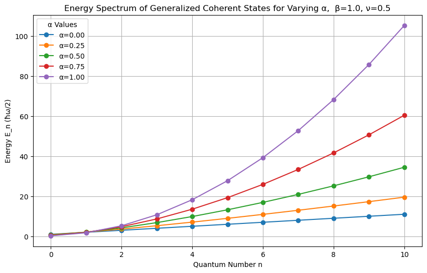
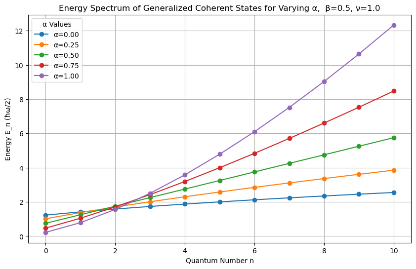
Figure 1: Energy spectra of generalized CS (2.10) as a function of quantum numbers $n$ for varying deformation parameter $\alpha$. The plots illustrate the influence of the parameter $\alpha$ on the energy eigenvalues $E_{n}$, with fixed values of $\beta$ and $\nu$. Each curve corresponds to a specific value of $\alpha$, demonstrating the deformation effects in the spectral structure

We can define the position and momentum operators, $\hat{q}_{\alpha,\beta,\nu}$ and $\hat{p}_{\alpha,\beta,\nu}$ respectively, for the generalized oscillator, concerning the creation and annihilation operators by:

$$\hat{q}_{\alpha,\beta,\nu}=\sqrt{\frac{\hbar}{2m\omega}}\left(A_{\alpha,\beta,\nu}+A^{\dagger}_{\alpha,\beta,\nu}\right);\,\,\,\,\,\hat{p}_{\alpha,\beta,\nu}=i\sqrt{\frac{\hbar m\omega}{2}}\left(A^{\dagger}_{\alpha,\beta,\nu}-A_{\alpha,\beta,\nu}\right).$$ (2.13)

Using the commutation rule (2.3), we obtain

$$\left[\hat{q}_{\alpha,\beta,\nu},\hat{p}_{\alpha,\beta,\nu}\right]=i\hbar[A_{\alpha,\beta,\nu}\,,\,A^{\dagger}_{\alpha,\beta,\nu}]=i\hbar\left([n+1]_{\alpha,\beta,\nu}-[n]_{\alpha,\beta,\nu}\right)$$ (2.14)

and the Deformed Heisenberg’s equations of motion:

$$\dot{\hat{q}}_{\alpha,\beta,\nu} = \left([n+1]_{\alpha,\beta,\nu}-[n]_{\alpha,\beta,\nu}+1\right)\frac{\hat{p}_{\alpha,\beta,\nu}}{2m};$$

$$\dot{\hat{p}}_{\alpha,\beta,\nu} = -\left([n+1]_{\alpha,\beta,\nu}-[n]_{\alpha,\beta,\nu}+1\right)\frac{\omega^{2}\hat{q}_{\alpha,\beta,\nu}}{2}$$ (2.15)

Definition 2.1.

Using $z^{n}\,\,\,(n=0,1,2...)$ as a basis function for this algebra, the three deformed boson operators assume the form

$$A^{\dagger}_{\alpha,\beta,\nu}:=\left(\sqrt{\frac{m\omega}{2\hbar}}z-\sqrt{\frac{\hbar}{2m\omega}}\hat{D}_{\alpha,\beta,\nu}\right),\,\,\,\,\,A_{\alpha,\beta,\nu}:=\left(\sqrt{\frac{m\omega}{2\hbar}}z+\sqrt{\frac{\hbar}{2m\omega}}\hat{D}_{\alpha,\beta,\nu}\right),$$

$$N=A^{\dagger}_{\alpha,\beta,\nu}A_{\alpha,\beta,\nu};$$ (2.16)

where the deformed boson $\mathcal{W}_{\alpha,\beta,\nu}$-derivative $\hat{D}_{\alpha,\beta,\nu}$ satisfies the relation

$$\hat{D}_{\alpha,\beta,\nu}z^{n} = [n]_{\alpha,\beta,\nu}z^{n-1}$$ (2.17)

$$= \frac{\Gamma(\beta n+1)}{\Gamma(\beta n+1-\alpha)}\frac{\Gamma(\beta n+1-\alpha+\nu)}{\Gamma(\beta(n-1)+1-\alpha+\nu)}z^{n-1}.$$ (2.18)

The $\mathcal{W}_{\alpha,\beta,\nu}$-coherent states $|z;\alpha,\beta,\nu\rangle$ are defined by the expression

$$|z;\alpha,\beta,\nu\rangle=[\mathcal{N}_{\alpha,\beta,\nu}(|z|^{2})]^{-1/2}\sum_{n=0}^{\infty}\frac{z^{n}}{\sqrt{[n]_{\alpha,\beta,\nu}!}}|n\rangle,\,\,\,\,\,z\in\mathbb{C};$$ (2.19)

with normalization $\mathcal{N}_{\alpha,\beta,\nu}(|z|^{2})=\Gamma(1-\alpha+\nu)\mathcal{W}_{\alpha,\beta,\nu}(|z|^{2})$, see [14] for more details about the $\mathcal{W}_{\alpha,\beta,\nu}$-function

$$\mathcal{W}_{\alpha,\beta,\nu}(x)=\sum_{n=0}^{\infty}\prod_{i=1}^{n}\frac{\Gamma(\beta i+1-\alpha)}{\Gamma(\beta i+1)}\frac{x^{n}}{\Gamma(\beta n+1-\alpha+\nu)}.$$

Remark 2.

if $z=x^{\beta}$ we have that the following fractional differential operator gives the $\mathcal{W}_{\alpha,\beta,\nu}$-derivative

$$\hat{D}_{\alpha,\beta,\nu}=x^{\alpha-\nu}\frac{d^{\beta}}{dx^{\beta}}x^{\nu}\frac{d^{\alpha}}{dx^{\alpha}}.$$ (2.20)

From the eq. (2.19), the probability of finding the state $|n>$ in the state ket $|z;\alpha,\beta,\nu>$ is equal to

$$p_{\alpha,\beta,\nu}(n,z)=\frac{\Gamma(1-\alpha+\nu)\left(|z|^{2}\right)^{n}}{\left(\prod_{i=1}^{n}\frac{\Gamma(\beta i+1)}{\Gamma(\beta i+1-\alpha)}\right)\Gamma(\beta n+1-\alpha+\nu)\mathcal{W}_{\alpha,\beta,\nu}(|z|^{2})}.$$ (2.21)

It coincides with the Poisson distribution characterizing the conventional CS for $\alpha=0,\,\beta=1,\,\nu=0$.

For two different complex numbers $z$ and $z^{\prime}$, the states $|z\rangle$ and $|z^{\prime}\rangle$ are, in general, not orthogonal and their overlap is given by

$$\langle z|z^{\prime}\rangle=\frac{\mathcal{N}_{\alpha,\beta,\nu}(z^{*}z^{\prime})}{\sqrt{\mathcal{N}_{\alpha,\beta,\nu}(|z|^{2})\cdot\mathcal{N}_{\alpha,\beta,\nu}(|z^{\prime}|^{2})}}$$

where $\mathcal{N}_{\alpha,\beta,\nu}(z^{*}z^{\prime})=\sum_{n=0}^{\infty}\frac{\left(z^{*}z^{\prime}\right)^{n}}{[n]_{\alpha,\beta,\nu}!}$.

2.1 Deformed harmonic oscillator

Considering the creation and annihilation operators defined in (2.1), and the equation related to the ground state $A^{\dagger}_{\alpha,\beta,\nu}|0\rangle=0$, we can find the analytical expression of the eigenfunction of the ground state by solving the fractional differential equation

$$\left(\sqrt{\frac{m\omega}{2\hbar}}z+\sqrt{\frac{\hbar}{2m\omega}}\hat{D}_{\alpha,\beta,\nu}\right)\langle z|0\rangle=0.$$

It is simple to show that the normalized ground state wave function assumes the form:

$$\langle z|0\rangle=\left(\frac{m\omega}{\pi\hbar}\right)^{\frac{1}{4}}\sum_{n=0}^{\infty}\frac{\left(-\frac{m\omega}{\hbar}\right)^{n}}{[2n]_{\alpha,\beta,\nu}!!}z^{2n},$$ (2.22)

where $[n]_{\alpha,\beta,\nu}!!$ is the generalized double factorial related to (2.1). To determine the eigenfunctions of the excited states, we can apply, recursively, the creation operator on the ground state $\langle z|n\rangle=\frac{1}{\sqrt{[n]_{\alpha,\beta,\nu}}}\left(A^{\dagger}_{\alpha,\beta,\nu}\right)^{n}|0\rangle$. For example, the first excited state is:

$$\langle z|1\rangle=\sqrt{\frac{m\omega}{2\hbar}}\frac{2z}{\sqrt{[1]_{\alpha,\beta,\nu}!}}\langle z|0\rangle.$$ (2.23)

Remark 3.

Obviously, for $\alpha=\nu=0$ and $\beta=1$, we obtain the eigenfunction of the classical harmonic oscillator.

Figure 2 illustrates the behavior of the ground state $\langle z|0\rangle$ and the first excited state $\langle z|1\rangle$ wavefunctions for different values of the deformation parameter $\nu$, under two distinct parameter sets ($\alpha=0,\beta=1$ and $\alpha=0.5,\beta=0.5$). The plots reveal how variations in $\nu$ influence the symmetry, amplitude, and spatial distribution of the wavefunctions, highlighting the effects of deformation on both ground and excited states.

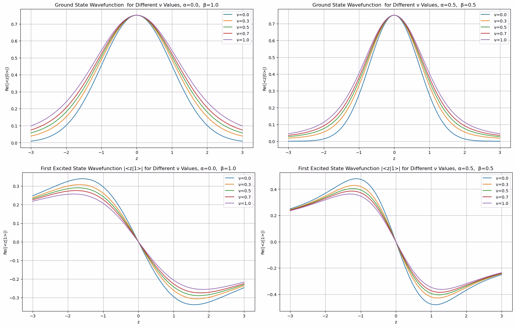
Figure 2: Ground states $\langle z|0\rangle$ and First excited states $\langle z|1\rangle$ for different values of the deformation parameters ($\alpha,\beta,\nu$). We set: $m=\omega=\hbar=1$

2.2 Continuity and completeness of $\mathcal{W}_{\alpha,\beta,\nu}$-coherent states

The states (2.19) are coherent if they are continuous in the label $z$. This condition follows from the joint continuity of the reproducing kernel $\mathcal{K}(z;z^{\prime})\equiv\langle z|z^{\prime}\rangle=\langle z^{\prime}|z\rangle^{*}$, in fact:

$$\||z^{\prime}\rangle-|z\rangle\|^{2}=\langle z^{\prime}|z^{\prime}\rangle+\langle z|z\rangle-2\Re{\langle z^{\prime}|z\rangle},$$ (2.24)

and is easily satisfied in practice.

The conditions of completeness, and hence the resolution of unity (1.1), imposes for $x\equiv|z|^{2}$ the equation

$$\int_{0}^{\infty}x^{n}\left[\pi\frac{U(x)}{\mathcal{N}_{\alpha,\beta,\nu}(x)}\right]dx=[n]_{\alpha,\beta,\nu}!.$$ (2.25)

(see [4] for details). The equation (2.25) is the Stieltjes moment problems of the unknown positive function $\tilde{U}(x)=\pi\frac{U(x)}{\mathcal{N}_{\alpha,\beta,\nu}(x)}$. It is important to note that not all deformed algebras lead to CS within the construction framework, as the moment problem (2.25) does not always have a solution, see [15],[16].

We know that strictly positive determinants of the Hankel-Hadamard matrices are necessary and sufficient for the weight function to exist [10],[15].

The not-trial Stieltjes problem can be tackled using a Mellin and inverse Mellin transforms approach, extending the natural value of $n$ to the complex values $s$ and rewriting (2.25) as

$$\int_{0}^{\infty}x^{s-1}\tilde{U}(x)dx=[s-1]_{\alpha,\beta,\nu}!.$$ (2.26)

Remark 4.

If $\alpha=0$, we obtain $[n]_{0,\beta,\nu}!=\frac{\Gamma(\beta n+1+\nu)}{\Gamma(1+\nu)}$ which is the generalized factorial performed by adopting the Mittag-Leffler function. If $\alpha=1$, $[n]_{1,\beta,\nu}!=\beta^{n}n!\frac{\Gamma(\beta n+\nu)}{\Gamma(\nu)}$ we have the generalized factorial in the case of the classical Wright function.

2.2.1 Resolution Of Unity

From the definition of the finite moments:

$$[n]_{\alpha,\beta,\nu}!=\left(\prod_{i=1}^{n}\frac{\Gamma(\beta i+1)}{\Gamma(\beta i+1-\alpha)}\right)\cdot\frac{\Gamma(\beta n+1-\alpha+\nu)}{\Gamma(1-\alpha+\nu)},$$

we aim to identify the conditions necessary for the existence of a measure corresponding to these moments. The moment sequence presented involves products of ratios of Gamma functions. To analyze the existence of a measure linked to these moments, it is essential to ensure that the moment sequence behaves appropriately, particularly in growth and positivity, while verifying the applicability of established conditions. Carleman’s condition offers a sufficient criterion for the determinacy of the moment problem. In the Appendix A, we provide a detailed analysis of Carleman’s condition concerning our finite moments $[n]_{\alpha,\beta,\nu}!$ Specifically, we find that the condition $\frac{\alpha+\beta}{2}\leq 1$ is sufficient to ensure that Carleman’s condition holds, thus confirming the uniqueness of the associated measure.[15]

2.3 Positive weight function in the Wright coherent states

The family of CS using the Mittag-Leffler functions has been deeply investigated by Sixdeniers and collaborators in [10]. The Wright function case has been analysed in [12] and [13]. In the following, we solve the Stieltjes problem in the case of Wright generalized factorial ($\alpha=1$), considering the following equation as the Melling transform for complex variable $s$, obtaining the same result given by Giraldi and Mainardi in [13]

$$\int_{0}^{\infty}x^{s-1}\tilde{U}_{1,\beta,\nu}(x)dx=[s-1]_{1,\beta,\nu}!=\beta^{s-1}\cdot\frac{\Gamma(s)\Gamma(\beta(s-1)+\nu)}{\Gamma(\nu)}.$$ (2.27)

To obtain $\tilde{U}_{1,\beta,\nu}(x)$, we have to carry out an inverse Mellin transform on (2.27).

$$\tilde{U}_{1,\beta,\nu}(x)=\frac{1}{\beta\Gamma(\nu)}\frac{1}{2\pi\imath}\int_{\mathcal{L}}\left(\frac{x}{\beta}\right)^{-s}\Gamma(s)\Gamma(\beta(s-1)+\nu)ds=\frac{1}{\beta\Gamma(\nu)}H_{0,2}^{2,0}\left[\frac{x}{\beta}\left|\begin{array}[]{ll}-\\ (0,1)\,\,,\,\,(\nu-\beta,\beta).\end{array}\right.\right]$$ (2.28)

that is the Fox-H function

$$H_{p,q}^{m,n}\left[z\left|\begin{array}[]{ll}(a_{1},A_{1}),...,(a_{p},A_{p})\\ (b_{1},B_{1}),...,(b_{q},B_{q})\end{array}\right.\right]=\frac{1}{2\pi\imath}\int_{\mathcal{L}}\frac{\prod_{j=1}^{m}\Gamma(b_{j}+B_{j}s)\prod_{j=1}^{n}\Gamma(1-a_{j}-A_{j}s)}{\prod_{j=m+1}^{q}\Gamma(1-b_{j}-B_{j}s)\prod_{j=n+1}^{p}\Gamma(a_{j}+A_{j}s)}z^{-s}ds.$$

Refer to [17],[18] for details about general theory and application of the H-function. Considering the relations (2.9.31)and (2.9.32) in [18], we can rewrite the equation (2.28) in the following integral form

$$\tilde{U}_{1,\beta,\nu}(x)=\frac{1}{\beta^{2}\Gamma(\nu)}\int_{0}^{\infty}t^{\frac{\nu}{\beta}-2}exp\left(-t^{\frac{1}{\beta}}-\frac{x}{\beta t}\right)dt.$$ (2.29)

2.3.1 Case $\alpha=\beta$

$$\int_{0}^{\infty}x^{s-1}\tilde{U}_{\beta,\beta,\nu}(x)dx=[s-1]_{\beta,\beta,\nu}!=\frac{\Gamma(\beta s+1-\beta)\Gamma(\beta(s-2)+1+\nu)}{\Gamma(1-\beta+\nu)}.$$ (2.30)

To obtain $\tilde{U}_{\beta,\beta,\nu}(x)$, we have to carry out an inverse Mellin transform on (2.30).

$$\tilde{U}_{\beta,\beta,\nu}(x)=\frac{1}{\Gamma(1-\beta+\nu)}\frac{1}{2\pi\imath}\int_{\mathcal{L}}x^{-s}\Gamma(\beta s+1-\beta)\Gamma(\beta(s-2)+1+\nu)ds$$ (2.31)

$$=\frac{1}{\Gamma(1-\beta+\nu)}H_{0,2}^{2,0}\left[\frac{x}{\beta}\left|\begin{array}[]{ll}-\\ (1-\beta,\beta)\,\,,\,\,(1-2\beta+\nu,\beta).\end{array}\right.\right]$$ (2.34)

2.3.2 Case $\alpha=1-\beta$

$$\int_{0}^{\infty}x^{s-1}\tilde{U}_{1-\beta,\beta,\nu}(x)dx=[s-1]_{1-\beta,\beta,\nu}!=\frac{\beta^{s-1}\Gamma(\beta)\Gamma(s)\Gamma(\beta s+\nu)}{\Gamma(\beta+\nu)\Gamma(\beta s)}.$$ (2.35)

To obtain $\tilde{U}_{1-\beta,\beta,\nu}(x)$, we have to carry out an inverse Mellin transform on (2.35).

$$\tilde{U}_{1-\beta,\beta,\nu}(x)=\frac{\Gamma(\beta)}{\beta\Gamma(\beta+\nu)}\frac{1}{2\pi\imath}\int_{\mathcal{L}}\left(\frac{x}{\beta}\right)^{-s}\frac{\Gamma(s)\Gamma(\beta s+\nu)}{\Gamma(\beta s)}ds$$ (2.36)

$$=\frac{\Gamma(\beta)}{\beta\Gamma(\beta+\nu)}H_{1,2}^{2,0}\left[\frac{x}{\beta}\left|\begin{array}[]{ll}(0,\beta)\\ (0,1)\,\,,\,\,(\nu,\beta).\end{array}\right.\right]$$ (2.39)

$$=\frac{\Gamma(\beta)}{\beta^{2}\Gamma(\beta+\nu)\Gamma(-\nu)}\int_{1}^{\infty}(t^{\frac{1}{\beta}}-1)^{-\nu-1}t^{\frac{1}{\beta}-1}e^{-\frac{x}{\beta}t}dt.$$ (2.40)

Other two subcases $[s]_{0,2r,0}!=\Gamma(2rs+1)$ and $[s]_{\beta,r,\beta}!=(\Gamma(rs+1))^{2}$ have been investigated by Penson et al. in [11]

3 Quantum Fluctuations of Quadrature

In quantum mechanics, characterising states through their quadrature operators provides crucial insights into the inherent uncertainties that govern their behaviour. Quadrature operators denoted here as $q_{\alpha,\beta,\nu}$ and $p_{\alpha,\beta,\nu}$ defined in (2.13), are fundamental in analyzing the properties of generalized CS, particularly regarding their fluctuations. These operators represent position and momentum-like variables and are defined as the corresponding annihilation and creation operators.

We rewrite the explicit forms of the quadrature operators:

$$q_{\alpha,\beta,\nu}=\sqrt{\frac{\hbar}{2m\omega}}\left(A_{\alpha,\beta,\nu}+A^{\dagger}_{\alpha,\beta,\nu}\right),\quad p_{\alpha,\beta,\nu}=i\sqrt{\frac{\hbar m\omega}{2}}\left(A^{\dagger}_{\alpha,\beta,\nu}-A_{\alpha,\beta,\nu}\right).$$ (3.1)

The expectation values of these operators are derived in terms of the state parameters, providing a foundation for calculating their variances, which quantify the quantum fluctuations. Specifically, we find:

$$\langle q_{\alpha,\beta,\nu}\rangle =\sqrt{\frac{\hbar}{2m\omega}}\left(\langle A_{\alpha,\beta,\nu}\rangle+\langle A^{\dagger}_{\alpha,\beta,\nu}\rangle\right),$$ (3.2)

$$\langle p_{\alpha,\beta,\nu}\rangle =i\sqrt{\frac{\hbar m\omega}{2}}\left(\langle A^{\dagger}_{\alpha,\beta,\nu}\rangle-\langle A_{\alpha,\beta,\nu}\rangle\right).$$ (3.3)

The fluctuations in the quadratures are quantified by the variances $\Delta q^{2}_{\alpha,\beta,\nu}$ and $\Delta p^{2}_{\alpha,\beta,\nu}$, which encapsulate the spread of the measurements around the mean values. In particular, we derive the relations for the variances as follows:

$$\Delta q^{2}_{\alpha,\beta,\nu} =\frac{\hbar}{2m\omega}\{[n+1]_{\alpha,\beta,\nu}-[n]_{\alpha,\beta,\nu}\},$$ (3.4)

$$\Delta p^{2}_{\alpha,\beta,\nu} =\frac{\hbar m\omega}{2}\{[n+1]_{\alpha,\beta,\nu}-[n]_{\alpha,\beta,\nu}\}.$$ (3.5)

In the vacuum state

$$(\Delta q^{2}_{\alpha,\beta,\nu})_{0} =\sqrt{\frac{\hbar}{2m\omega}[1]_{\alpha,\beta,\nu}},$$ (3.6)

$$(\Delta p^{2}_{\alpha,\beta,\nu})_{0} =\sqrt{\frac{\hbar m\omega}{2}[1]_{\alpha,\beta,\nu}}.$$ (3.7)

These results culminate in the expression of the product of the uncertainties, which adheres to the Heisenberg uncertainty principle:

$$\Delta q_{\alpha,\beta,\nu}\Delta p_{\alpha,\beta,\nu}=\frac{\hbar}{2}\{[n+1]_{\alpha,\beta,\nu}-[n]_{\alpha,\beta,\nu}\}.$$ (3.8)

Finally, we express the uncertainty relation for our CS in terms of the generalized gamma functions, emphasizing the dependence on the state parameters:

$$\Delta q_{\alpha,\beta,\nu}\Delta p_{\alpha,\beta,\nu}=\frac{\hbar}{2}\left[\frac{\Gamma(\beta(n+1)+1)}{\Gamma(\beta(n+1)+1-\alpha)}\frac{\Gamma(\beta(n+1)+1-\alpha+\nu)}{\Gamma(\beta n+1-\alpha+\nu)}-\frac{\Gamma(\beta n+1)}{\Gamma(\beta n+1-\alpha)}\frac{\Gamma(\beta n+1-\alpha+\nu)}{\Gamma(\beta(n-1)+1-\alpha+\nu)}\right]\\ \quad n\geq 1.$$ (3.9)

This analysis not only elucidates the quantum fluctuations present in generalized CS but also underscores the interplay between the state parameters and the fundamental limits imposed by quantum mechanics. Through this framework, we gain valuable insights into the nature of quantum noise and its implications for quantum technologies. As shown in Figure 3, 4, the product of the uncertainties of the vacuum state

$$\left(\Delta q_{\alpha,\beta,\nu}\right)_{0}\left(\Delta p_{\alpha,\beta,\nu}\right)_{0}=\frac{\hbar}{2}[1]_{\alpha,\beta,\nu}=\frac{\hbar}{2}\frac{\Gamma(\beta+1)}{\Gamma(\beta+1-\alpha)}\frac{\Gamma(\beta+1-\alpha+\nu)}{\Gamma(1-\alpha+\nu)};$$ (3.10)

depends on the parameters $\alpha$, $\beta$, and $\nu$. It shows that in the case $\alpha=0$ (Figure 3(a)), the uncertainty relation of the vacuum state goes from a value of $\frac{\hbar}{2}$ to $\hbar$ representing a higher level of quantum noise or fluctuations than the standard coherent state.

(a) Mittag-Leffler case: $\alpha=0$

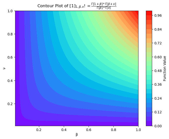
(b) Wright function case: $\alpha=1$

Figure 3: Visualization of quantum fluctuations in quadrature uncertainties of the vacuum state for the generalized deformed states, expressed in units of $\hbar/2$, illustrating the dependence of the uncertainty relation (Equation 3.10) on the parameters $\alpha$, $\beta$, and $\nu$.

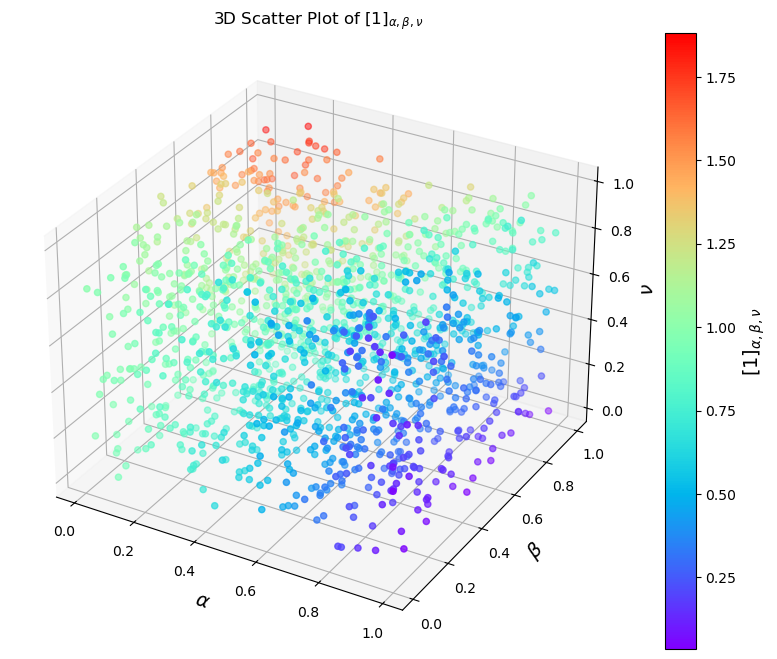
Figure 4: 3D scatter plot illustrating the dependency of the gamma ratio $[1]_{\alpha,\beta,\nu}=\frac{\Gamma(\beta+1)}{\Gamma(\beta+1-\alpha)}\frac{\Gamma(\beta+1-\alpha+\nu)}{\Gamma(1-\alpha+\nu)}$ on the parameters $\alpha$, $\beta$, and $\nu$ within the range $(0,1)$. The colour scale represents the computed gamma ratio values, highlighting variations across the parameter space.

4 Mandel parameter

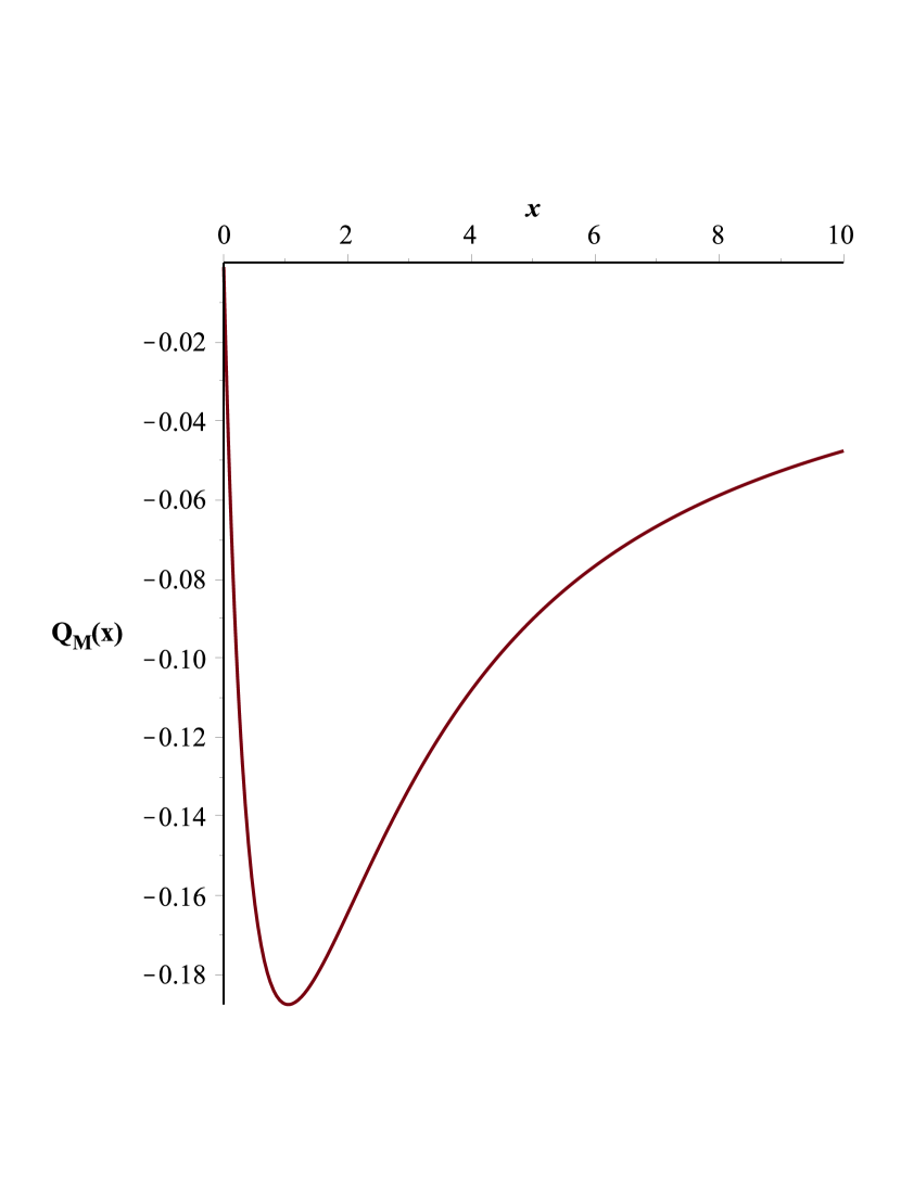
Figure 5: Plot of the Mandel parameter $Q_{M}(x)$ as a function of $x=|z|^{2}$, in the case of $\alpha=0,\beta=1,\,\nu=-1/2$. Mittag-Leffler function $E_{1,\frac{1}{2}}(x)$

.

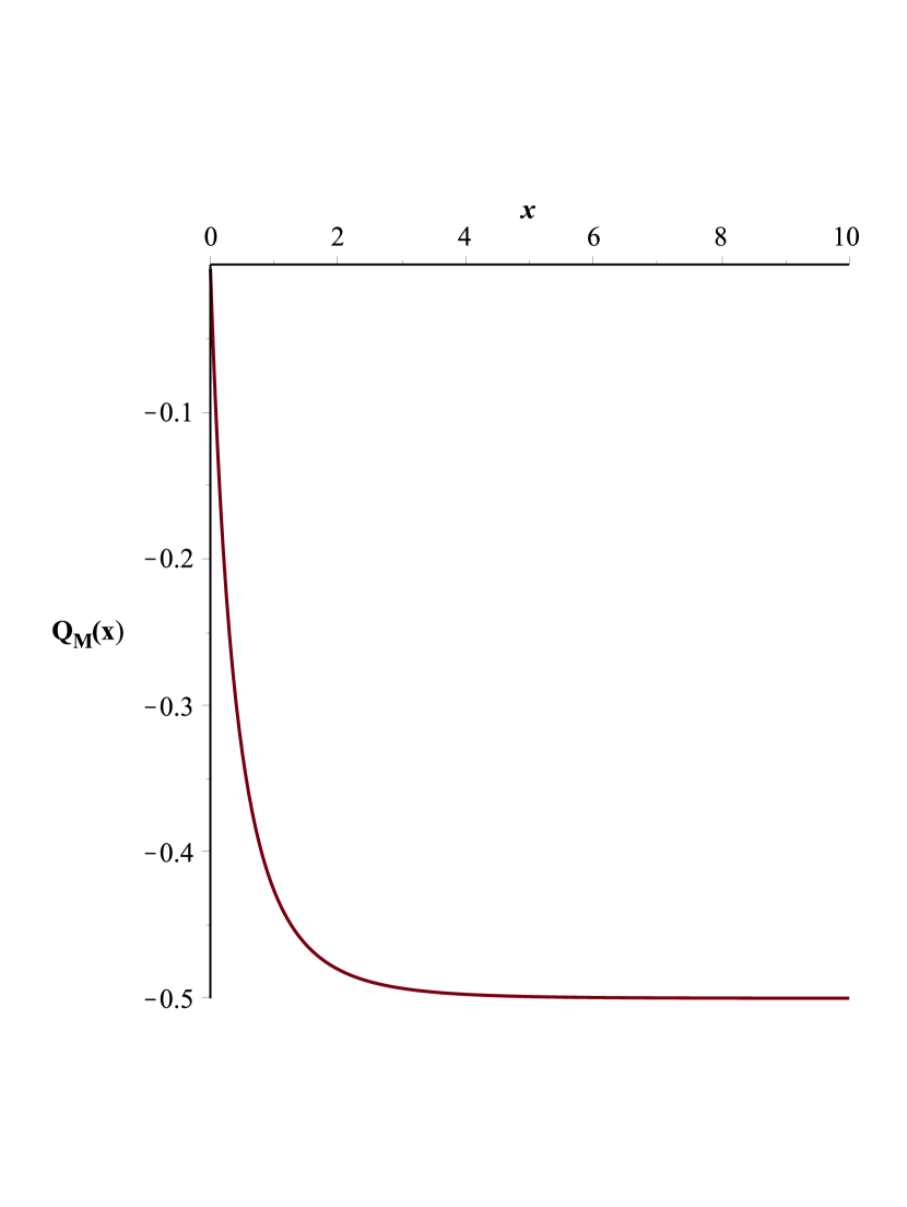
Figure 6: Plot of the Mandel parameter $Q_{M}(x)$ as a function of $x=|z|^{2}$, in the case of $\alpha=1,\beta=1,\,\nu=1/2$. Wright function $W_{1,\frac{1}{2}}(x)$.

While Glauber CS conventionally describes an ideal laser’s states, real lasers do not strictly conform to this model. In particular, the photon number statistics of real lasers deviate from a Poissonian distribution, often due to various nonlinear interactions that lead to distinct departures from the ideal case. Recently, deformations of the commutation rules of boson operators have been proposed to model physical systems that derive from these idealized behaviours [19], [20]. The real laser problem was addressed in this phenomenological context, demonstrating that CS of deformed boson operators provide a more accurate model for non-ideal lasers, particularly concerning photon number statistics. A Poisson distribution is characterized by the variance of the number operator $N$ being equal to its average. The deviation from the Poisson distribution can be measured with the Mandel parameter $Q_{M}(x)$, $(x=|z|^{2})$ [21]

$$Q_{M}=\frac{<N^{2}>-<N>^{2}}{<N>}-1.$$ (4.1)

Using the relation between various expectation values of polynomial Hermitian operators and the derivative of $\mathcal{N}_{\alpha,\beta,\nu}(|z|^{2})$, see also ref. [4]

$$<(A^{\dagger}_{\alpha,\beta,\nu})^{r}A^{r}_{\alpha,\beta,\nu}>=\frac{|z|^{2r}}{\mathcal{N}_{\alpha,\beta,\nu}(|z|^{2})}\left(\frac{d}{d|z|^{2}}\right)^{r}\mathcal{N}_{\alpha,\beta,\nu}(|z|^{2}),\,\,\,\,\,r=0,1,2,...\,.$$ (4.2)

We have the following expectation values computed over the generalized CS $|z;\alpha,\beta,\nu>$:

$$<A^{\dagger}_{\alpha,\beta,\nu}A_{\alpha,\beta,\nu}>=\frac{|z|^{2}}{\mathcal{W}_{\alpha,\beta,\nu}(|z|^{2})}\sum_{n=0}^{\infty}\prod_{i=1}^{n+1}\frac{\Gamma(\beta i+1-\alpha)}{\Gamma(\beta i+1)}\frac{(n+1)|z|^{2n}}{\Gamma(\beta(n+1)+1-\alpha+\nu)};$$ (4.3)

$$<(A^{\dagger}_{\alpha,\beta,\nu})^{2}A_{\alpha,\beta,\nu}^{2}>=\frac{|z|^{4}}{\mathcal{W}_{\alpha,\beta,\nu}(|z|^{2})}\sum_{n=0}^{\infty}\prod_{i=1}^{n+2}\frac{\Gamma(\beta i+1-\alpha)}{\Gamma(\beta i+1)}\frac{(n+1)(n+2)|z|^{2n}}{\Gamma(\beta(n+2)+1-\alpha+\nu)}.$$ (4.4)

For the $\mathcal{W}_{\alpha,\beta,\nu}$-coherent states (2.19), the corresponding Mandel $Q_{z}$ parameter can be evaluated via the expectation values which are listed above and via the expression below

$$Q_{z}=\frac{<(A^{\dagger}_{\alpha,\beta,\nu})^{2}A_{\alpha,\beta,\nu}^{2}>-\left(<A^{\dagger}_{\alpha,\beta,\nu}A_{\alpha,\beta,\nu}>\right)^{2}}{<A^{\dagger}_{\alpha,\beta,\nu}A_{\alpha,\beta,\nu}>}.$$ (4.5)

Negative values of the Mandel factor ($-1<Q_{z}<0$) (see Figures 6 and 6) indicate the non-classical nature of the states, revealing the sub-Poissonian photon number statistic, a phenomenon with a non-classical analogue. For further details, see [21].

5 Conclusion

In this study, we introduced a novel class of coherent states, denoted as $\mathcal{W}_{\alpha,\beta,\nu}$-coherent states, derived from a deformed boson algebra incorporating advanced mathematical structures such as the Mittag-Leffler and Wright functions. These coherent states were constructed using a generalized factorial $[n]_{\alpha,\beta,\nu}!$, enabling a broader exploration of quantum states and extending their applicability in quantum optics and fractional quantum mechanics. We demonstrated these states’ continuity and completeness, fulfilling the unity condition’s resolution through a Stieltjes moment problem, successfully addressed via the Mellin and inverse Mellin transforms. The analysis of quantum fluctuations in quadrature operators revealed an intricate dependence on the deformation parameters $(\alpha,\beta,\nu)$, with explicit derivations highlighting their impact on position and momentum uncertainties. Additionally, the Mandel parameter analysis underscored the non-classical properties of these states, revealing sub-Poissonian photon statistics in specific parameter regimes. These results suggest that $\mathcal{W}_{\alpha,\beta,\nu}$-coherent states are robust tools for describing quantum systems where standard coherent states fall short. The asymptotic analysis of the generalized factorials, as shown in the Appendix, further validated the consistency of our results, satisfying Carleman’s condition under specific parameter constraints. These findings expand the mathematical framework of coherent states and provide potential avenues for experimental realization in systems exhibiting fractional or non-linear dynamics. Future work may focus on exploring practical implementations of these states in quantum information systems and extending this formalism to other non-trivial algebraic structures.

6 Appendix A

Let’s analyze the asymptotic behavior of the generalized factorial

$$[n]_{\alpha,\beta,\nu}!=\left(\prod_{i=1}^{n}\frac{\Gamma(\beta i+1)}{\Gamma(\beta i+1-\alpha)}\right)\frac{\Gamma(\beta n+1-\alpha+\nu)}{\Gamma(1-\alpha+\nu)}.$$

We can break this generalized factorial into two parts: The product term:

$$P(n)=\prod_{i=1}^{n}\frac{\Gamma(\beta i+1)}{\Gamma(\beta i+1-\alpha)}.$$

The final term:

$$F(n)=\frac{\Gamma(\beta n+1-\alpha+\nu)}{\Gamma(1-\alpha+\nu)}.$$

We’ll analyze the asymptotic behaviour of each part separately. For large $x$, Stirling’s approximation for the Gamma function is given by:

$$\Gamma(x)\sim\sqrt{2\pi x}\left(\frac{x}{e}\right)^{x}.$$

We will apply this approximation to each Gamma term in both $P(n)$ and $F(n)$. Each term in the product can be approximated using Stirling’s formula. For large $i$, we approximate:

$$\Gamma(\beta i+1)\sim\sqrt{2\pi(\beta i+1)}\left(\frac{\beta i+1}{e}\right)^{\beta i+1},$$

and

$$\Gamma(\beta i+1-\alpha)\sim\sqrt{2\pi(\beta i+1-\alpha)}\left(\frac{\beta i+1-\alpha}{e}\right)^{\beta i+1-\alpha}.$$

Thus, each ratio becomes

$$\frac{\Gamma(\beta i+1)}{\Gamma(\beta i+1-\alpha)}\sim\frac{\left(\beta i+1\right)^{\beta i+1}}{\left(\beta i+1-\alpha\right)^{\beta i+1-\alpha}}\sim e^{-\alpha}(\beta i)^{\alpha}.$$

Therefore, the product becomes

$$P(n)\sim\prod_{i=1}^{n}e^{-\alpha}(\beta i)^{\alpha}=e^{-\alpha n}(\beta^{n}\,n!)^{\alpha}\sim e^{-\alpha n}(\beta\,n)^{\alpha n}.$$

Next, consider the final factor $F(n)$. Using Stirling’s approximation for large $n$:

$$\Gamma(\beta n+1-\alpha+\nu)\sim\sqrt{2\pi(\beta n+1-\alpha+\nu)}\left(\frac{\beta n+1-\alpha+\nu}{e}\right)^{\beta n+1-\alpha+\nu}.$$

Thus, for large $n$,

$$F(n)\sim\frac{\left(\beta n+1-\alpha+\nu\right)^{\beta n+1-\alpha+\nu}}{\Gamma(1-\alpha+\nu)}e^{-(\beta n+1-\alpha+\nu)}\sim e^{-\beta n}(\beta\,n)^{\beta n}.$$

Combining the two asymptotic behaviours from $P(n)$ and $F(n)$, we get the overall behaviour of the generalized factorial. Ignoring constants and focusing on the dominant growth, we have the following,

$$[n]_{\alpha,\beta,\nu}!\sim e^{-(\alpha+\beta)n}\cdot(\beta\,n)^{(\alpha+\beta)n}.$$

6.1 Carleman’s Condition for Stieltjes Moment Problem

Consider the moments defined by

$$m_{n}=e^{-(\alpha+\beta)n}\cdot(\beta\,n)^{(\alpha+\beta)n},$$

where $\alpha$ and $\beta$ are constants. We will analyze Carleman’s condition for the Stieltjes moment problem. To check whether the Carleman’s condition is satisfied, we need to evaluate the series:

$$\sum_{n=1}^{\infty}m_{n}^{-\frac{1}{2n}}.$$

In our case, we can find:

$$m_{n}^{-\frac{1}{2n}}=\left(e^{-(\alpha+\beta)n}\cdot(\beta\,n)^{(\alpha+\beta)n}\right)^{-\frac{1}{2n}}=e^{\frac{(\alpha+\beta)}{2}}\cdot(\beta\,n)^{-\frac{(\alpha+\beta)}{2}}.$$

Now, we want to consider the series:

$$\sum_{n=1}^{\infty}e^{\frac{(\alpha+\beta)}{2}}\cdot(\beta\,n)^{-\frac{(\alpha+\beta)}{2}}=e^{\frac{(\alpha+\beta)}{2}}\beta^{-\frac{(\alpha+\beta)}{2}}\cdot\sum_{n=1}^{\infty}n^{-\frac{(\alpha+\beta)}{2}}.$$

This series is a $p$-series and converges or diverges depending on the value of $\frac{(\alpha+\beta)}{2}$:

• Divergence: If $\frac{\alpha+\beta}{2}\leq 1$, the series diverges.

• Convergence: If $\frac{\alpha+\beta}{2}>1$, the series converges.

Finally, using Carleman’s condition for the Stieltjes moment problem, we can summarize that:

• If $\frac{\alpha+\beta}{2}\leq 1$, then

  $$\sum_{n=1}^{\infty}m_{n}^{-\frac{1}{2n}}=\infty,$$

  implying that the moment problem is determinate, and a unique positive measure exists and corresponds to the moments $m_{n}$.

• If $\frac{\alpha+\beta}{2}>1$the moment problem is indeterminate, a unique measure may not exist corresponding to the moments.

References

- [1] Schrödinger, E. (1926). Der stetige Übergang von der Mikro-zur Makromechanik. Naturwissenschaften, 14(28), 664-666.
- [2] Glauber, R. J. (1963). The quantum theory of optical coherence. Physical Review, 130(6), 2529–2539. https://doi.org/10.1103/PhysRev.130.2529
- [3] Klauder, J. R. (1963). Continuous‐representation theory. I. Postulates of continuous‐representation theory. Journal of Mathematical Physics, 4(8), 1055-1058.
- [4] Klauder, J. R., Penson, K. A., Sixdeniers, J. M. (2001). Constructing coherent states through solutions of Stieltjes and Hausdorff moment problems. Physical Review A, 64(1), 013817.
- [5] Gazeau, J. P., Baldiotti, M. C., Gitman, D. M. (2010). Coherent state quantization and moment problem. Acta Polytechnica 50(3)
- [6] Katriel, J., Solomon, A. I. (1991). Generalized q-bosons and their squeezed states. Journal of Physics A: Mathematical and General, 24(9), 2093.
- [7] Klauder, J.R., Skagerstam Be Sture, Coherent States, Application in Physics and Mathematical Physics (World Scientific, Singapore, 1985)
- [8] Penson, K. A., Solomon, A. I., J. Math. Phys. 40, 2354 (1999)
- [9] Sixdeniers, J-M., Penson, K. A., J.Phys. A. 33, 2907 (2000); 34, 2859 (2001)
- [10] Sixdeniers, J. M., Penson, K. A., Solomon, A. I. (1999). Mittag-Leffler coherent states. Journal of Physics A: Mathematical and General, 32(43), 7543.
- [11] Penson, K. A., Blasiak, P., Duchamp, G.H.E., Horzela, A., Solomon, A. I. (2009). On certain non-unique solutions of the Stieltjes moment problem. Discrete Mathematics & Theoretical Computer Science, 12.
- [12] Garra, R., Giraldi, F., Mainardi, F. (2019). Wright-type generalized coherent states. WSEAS Trans. Math, 18, 428-431.
- [13] Giraldi, F., Mainardi, F. Truncated generalized coherent states, J. Math. Phys. 64, 032105 (2023)
- [14] Droghei, R. (2021). On a Solution of a Fractional Hyper-Bessel Differential Equation using a Multi-Index Special Function. Fract Calc Appl Anal 24, 1559–1570. https://doi.org/10.1515/fca-2021-0065
- [15] Akhiezer, N. I. (1965). The classical moment problem and some related questions in analysis. Society for Industrial and Applied Mathematics.
- [16] Shohat, J., Tamarkin, J. (1943). The Problem of Moments (APS, New York)
- [17] Mathai, A. M., Saxena, R. K., Haubold, H. J. (2009). The H-function: theory and applications. Springer Science and Business Media.
- [18] Kilbas, A. A. (2004). H-transforms: Theory and Applications. CRC Press.
- [19] Katriel, J., Solomon, A. I. (1994). Nonideal lasers, nonclassical light, and deformed photon states. Phys. Rev. A 49, 5149.
- [20] Solomon, A. I. (1994). A characteristic functional for deformed photon phenomenology. Physics Letters A 196(1-2), 29-34
- [21] Mandel, L., Wolf, E. (1995). Optical Coherence and Quantum Optics (Cambridge University Press, Cambridge)