[table]capposition=top
Probabilistic Forecasts of Load, Solar and Wind for Electricity Price Forecasting
Abstract
Electricity price forecasting is a critical tool for the efficient operation of power systems and for supporting informed decision-making by market participants. This paper explores a novel methodology aimed at improving the accuracy of electricity price forecasts by incorporating probabilistic inputs of fundamental variables. Traditional approaches often rely on point forecasts of exogenous variables such as load, solar, and wind generation. Our method proposes the integration of quantile forecasts of these fundamental variables, providing a new set of exogenous variables that account for a more comprehensive representation of uncertainty. We conducted empirical tests on the German electricity market using recent data to evaluate the effectiveness of this approach. The findings indicate that incorporating probabilistic forecasts of load and renewable energy source generation significantly improves the accuracy of point forecasts of electricity prices. Furthermore, the results clearly show that the highest improvement in forecast accuracy can be achieved with full probabilistic forecast information. This highlights the importance of probabilistic forecasting in research and practice, particularly that the current state-of-the-art in reporting load, wind and solar forecast is insufficient.
Index Terms:
Electricity price forecasting, power market, probabilistic inputs, load, renewable energy sources, residual loadI Introduction and motivation
The energy sector has become more dynamic in recent years as renewable energy sources (RES) continue to expand and integrate into the existing infrastructure to meet the European Union’s (EU) 2050 carbon neutrality target. At the same time, market participants are faced with the issue of sector coupling, e.g. through electric vehicles and combined heat and power systems, making the role of energy forecasting even more important in the coming decades [1, 2].
As the EU continues to push for a significant increase in the share of renewable energy in the energy mix, price uncertainty continues to grow. The 2023 figures show that 45 of Germany electricity needs are now covered by renewables (31% wind, 12% solar, 2% others RES). But wind and solar generation are driven by the weather. For instance, on some days the RES cover 95% of the national demand for electricity (i.e. 29.12.2023), whereas on other the production drops below 7% (i.e. 30.11.2023).
On the demand side, instead of expanding infrastructure, utilities can try to slow the growth of peak demand through demand-side management (DSM), i.e., changing end-users’ electricity consumption patterns through regulation, financial incentives, or social pressure. However, as a result of the increased market share of RES and active DSM, the behavior of agents becomes more unpredictable, sudden drops in generation and consumption are more likely to occur, imbalances increase, and the electricity price becomes more volatile [3, 4]. Under such conditions, electricity price forecasting (EPF) becomes a real challenge [5], and models built a few years ago no longer provide accurate predictions. This situation calls for the development of innovative forecasting methods that go beyond the state of the art and meet the very demanding requirements of today’s electricity markets.
Recent empirical findings indicate that incorporating forecasts of fundamental variables, such as electricity demand or solar and wind generation, into EPF models tends to significantly outperform architectures without these variables [6, 7, 8]. However, to our knowledge, the use of fundamental variables in EPF has been limited to point predictions.
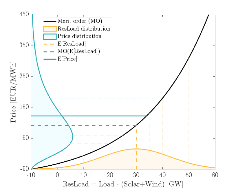
In this study, we argue that not only point forecasts of fundamental variables, but also probabilistic forecasts should be included in electricity price forecasting models. The relevance of probabilistic inputs in electricity price forecasting models is well justified by fundamental theory: The electricity price results from the intersection of the supply and demand curves, which are usually non-linear curves, [9, 10]. Fig. 1 shows an illustrative example of a supply stack model with a non-linear merit order (MO) curve depending on the residual load (ResLoad), which is the load minus solar and wind generation. Here, in a deterministic setting, a ResLoad of 30GW leads to an electricity price of . If the ResLoad is uncertain (as it is in day-ahead markets) with a density centred around 30GW as shown in Fig. 1, then the electricity price also becomes uncertain (a random variable) with the resulting cyan coloured density as shown on the y-axis. However, the expected value of this cyan electricity price density is approximately . This is significantly higher than the point forecast plugged into the merit order . Thus, to properly derive the expected electricity price, the full distribution of the residual load, or more generally the distribution of the electricity load, such as solar and wind generation, is required. Thus, our fundamental theory leads us directly to use probabilistic forecasts of load and RES to derive accurate point forecasts of electricity prices.
In this paper we design a model that includes – in addition to the standard set of regressors – a set of quantile forecasts of fundamental variables. To estimate the models, we use the Least Absolute Shrinkage and Selection Operator (LASSO) [11], which allows us to consider an almost unlimited number of explanatory variables [12]. Our empirical tests, performed on the German electricity market, show that the integration of probabilistic inputs significantly improves the accuracy of electricity price forecasts. The proposed methods outperform the standard approach by up to 13 %.
The reminder of this paper is structured as follows. In Section II we present the datasets, then in Section III we explain how the probabilistic forecasts of fundamental variables are computed and how they are included in the the day-ahead electricity prices forecasting models. In Section IV we discuss the obtained results in terms of the root mean square error (RMSE) and the test for Conditional Predictive Ability (CPA) of Giacomini and White [13]. We conclude Section IV with the analysis of the most frequently selected variables. Finally, in Section V we summarize the main results.
II Data
In this study, we used publicly available data from Transparency ENTSO-E (https://transparency.entsoe.eu) for the German energy market. Specifically we used day-ahead prices for German-Luxemburg bidding zone111Can be accessed from ENTSO-E: Transmission Day-ahead Prices with code BZNDE-LU. Note that the bidding zone also includes Austria (BZNDE-AT-LU) but only until 09/30/2018 and the day-ahead forecasts and actual observations of load, solar and wind generation in Germany222Can be accessed from ENTSO-E with code CTYDE. Note that we aggregate the values for onshore and offshore wind into one time series. In addition, we used data from Investing.com (https://www.investing.com) for the closing prices of API2 (coal), Title Transfer Facility (TTF; natural gas), Brent (crude oil) and European Union Allowance (EUA; carbon emissions).
Note that some of the collected data are available at 15-minute resolution, so we have aggregated them into hourly time series to unify the data set. All hourly series are then further pre-processed to account for the time changes to and from Daylight Saving Time. Missing values that occur during the transition from Central European Time (CET) to Central European Summer Time (CEST) are replaced by the arithmetic mean of the observations from the surrounding hours. Double values occurring during the transition back from CET are replaced by their arithmetic mean.
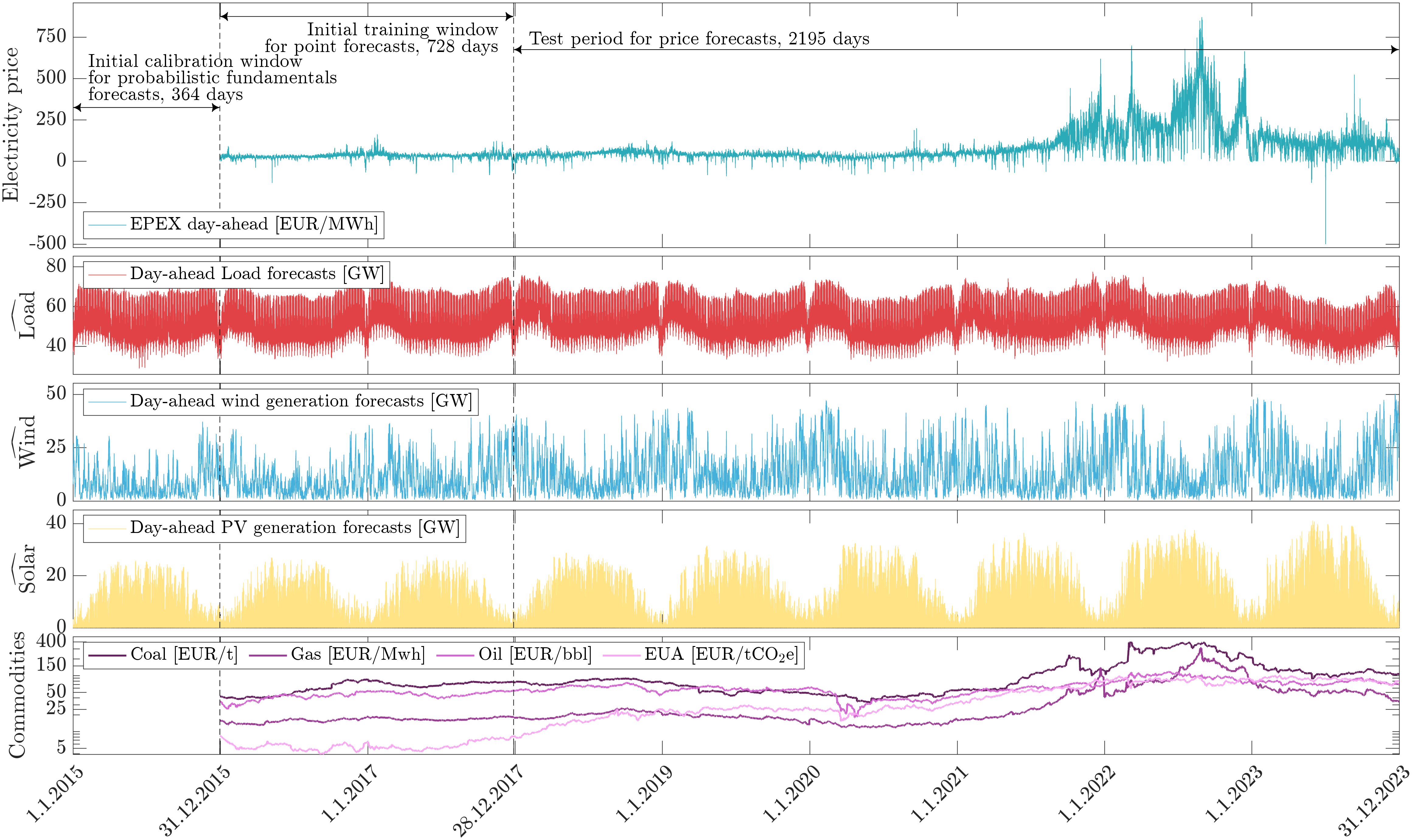
All collected time series span from 1.1.2015 to 31.12.2023, with a 6-year out-of-sample test period starting at 28.12.2017, as shown in Fig. 2. To obtain the forecast, we use a rolling window scheme. First, we use a 364-day (52 weeks, ca. one year) rolling calibration window to compute the probabilistic forecast of the fundamental variables for the period from 31.12.2015 to 31.12.2023. Once the probabilistic forecast is available, another rolling calibration window of 728 days is introduced to estimate the price forecasting models. For example, to obtain the electricity price forecast for all 24 hours of 29.12.2017, we use the collected time series together with the obtained probabilistic forecast for the period from 31.12.2015 to 28.12.2017, then the calibration window is shifted by one day (1.1.2016-29.12.2017 and the forecast for 30.12.2017 is obtained. The procedure is repeated until the last day of the out-of-sample period is obtained.
III Methodology
III-A Postprocessing of fundamental point predictions
The publicly available data provides point predictions of day-ahead load, solar, and wind generation forecasts. To use the probabilistic forecasts of these variables as inputs to the electricity price forecasting models, we must first construct them. This is done using a postprocessing technique that allows us to convert point forecasts into quantile forecasts [14]. Although there are several well-established postprocessing techniques, we have chosen to compare two approaches: historical simulation and quantile regression.
Before describing the methods, we would like to point out that due to the significant seasonality of solar power generation, which can lead to estimation inaccuracies, we have chosen not to construct a probabilistic forecast when the day-ahead point forecast is equal to zero (). Furthermore, the postprocessing methods themselves do not impose any restrictions on the quantile forecast being non-negative. Therefore, for variables that theoretically cannot take negative values, we decided to truncate them to zero.
In addition, we would like to point out that both historical simulation and quantile regression require access to actual observations of the fundamental variable of interest. It is important to keep in mind that at the beginning of day (at the moment of forecasting day ), we only have access to actual observations up to day (see Fig. 3). Taking this into account, we calibrate the model and obtain the empirical quantile of the errors ( for HS in eq. 1) or coefficients and (for QR in eq. 2) we use data from to ( in the length of the calibration window size, here ).

Finally, let us remark that we have applied the proposed postprocessing techniques to obtain probabilistic forecasts of system load, solar and wind power generation, as well as a linear combination of these, namely RES (Solar+Wind) and ResLoad (Load - RES).
III-A1 Probabilistic forecasting by historical simulation
The historical simulation (HS) method is a straightforward approach. We begin by computing the empirical quantile of the point prediction error on the training set, see Fig. 2. This value is then added to the point prediction to obtain the quantile prediction of for day and hour :
| (1) |
where is a probability level, is the actual observation of given fundamental variable for day and hour and is corresponding day-ahead point forecast.
III-A2 Probabilistic forecasting by quantile regression
Quantile regression (QR) is a method that has been used successfully in many forecasting applications [15, 16, 17, 18, 19, 20]. This approach estimates conditional quantiles of the target variable as a linear combination of point forecasts in a quantile regression setting [21]:
| (2) |
where is the conditional th quantile and are coefficients that are estimated independently for each quantile and each hour of a day by minimizing so-called check function:
| (3) |
with quantile loss .
Note that the numerical inefficiency of quantile regression can result in overlapping neighboring percentiles, leading to a quantile crossing problem [22]. To address this, following [23] the quantiles are sorted to obtain monotonic quantile curves, independently for each day and hour.
III-A3 ReLU-based transformation
Furthermore, for benchmarking purposes, we apply nonlinear transformations of the forecasts. To ensure that the improvement in forecast accuracy is due to the use of probabilistic forecasts and not simply the introduction of a nonlinearity in the model, we apply the following transformation:
| (4) |
where is an empirical -quantile of day-ahead forecast of given fundamental variable from the calibration window.
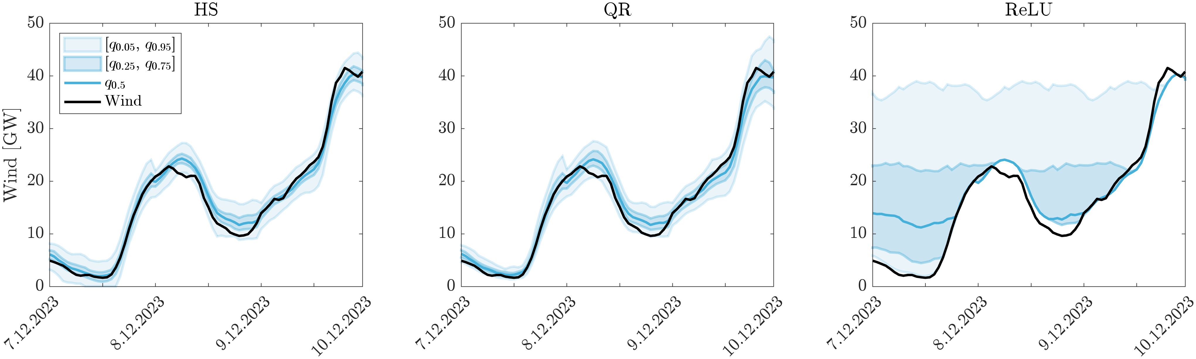
Note that unlike the other two approaches, the ReLU-based method does not produce the quantile prediction of (see Fig. 4). Instead, it produces a nonlinear transformation of the empirical quantiles of . This means that unlike and , the expression is not the quantile prediction. Keep in mind that the value of is calculated using only the historical data on the forecasts of , without the necessity of an actual observation of , so it is derived using the entire calibration window from day to .
III-B Base Models
III-B1 Expert model
The day-ahead electricity price forecasts are obtained through the application of two distinct model classes. The first is a parsimonious linear model which contains autoregressive information with exogenous variables (later referred to as the Expert model). Various version of this model were used in a number of EPF studies under different names and abbreviations (see, for example, [24, 25, 26, 27, 28]). The electricity price for day and hour is given by the following formula:
| (5) |
where the first three regressors capture the autoregressive effects of the prices for the same hour on days , and , provides information on the last known price, i.e, midnight of day , and stand for the maximum and minimum price of the previous day, , and stand for the day-ahead forecasts of system-wide load, solar and wind generation respectively. The next four variables represent the last observed market prices (i.e., the closing price of day ) for coal, gas, oil, and carbon emission allowances (EUAs). Finally, are daily dummies and is the noise term.
III-B2 High-dimensional linear model
The second model class is a parameter-rich high-dimensional linear model (HLM) introduced to the EPF literature by [29] and [30], and later used and modified in several EPF studies (for example [31, 32, 33, 28]). As this model type is often (also here) estimated using LASSO, literature calls this LEAR (LASSO Estimated AutoRegressive model)333Since both Expert and HLM models are estimated using LASSO, we want to avoid the LEAR notation..
| (6) |
The over 200-variable structure of this model allows all cross-hour dependencies to be included in the price forecasts.
Note that to avoid overfitting, the are excluded from for both Expert and HLM models for hours where more than 25% of the observations in the calibration window are equal to 0.
III-C Proposed extensions
In this study, we propose to include in forecasting models additional information that addresses the uncertainty of fundamental variables. The idea is to incorporate quantile forecasting of fundamental variables into the model structure:
| (7) |
where BaseModel indicates the model structure of either an Expert (Eq. (5)) or HLM-type (Eq. (6)) model, is a set of fundamental variables included in the model, is a set of considered probability levels and refers to one of the postprocessing methods.
We considered several variants of our approach depending on several factors. Let us now briefly describe all the features that define a given model. First, as already described in Section III-A, we consider two different postprocessing methods to obtain the quantile forecast of the fundamental variables: historical simulation and quantile regression averaging . Alternatively, the postprocessing technique can be replaced by a ReLU-based nonlinear transformation to obtain .
Second, we consider different sets of fundamental variables to be input into the model. To be more specific, we define seven different sets motivated by plausible fundamental modeling perspective in electricity markets.
-
1-3
The first three are one-element sets, where we include in the model the quantile forecast of either , , or , but only one at a time.
-
4
Second, we consider another one-element set, but already using the information of two variables, namely
-
5-7
The last three variants include information about all three considered fundamental variables, but with different levels of aggregation. We consider a one-element set including the residual load (), a two-element set consisting of Load and RES , and finally a three-element set .
Next, we consider seven sets of incorporated probability levels represented by . In particular, we compare the predictive performance of models that include different number of quantile prediction for given fundamental variable:
-
,
-
,
-
,
-
,
-
,
-
,
-
,
where ( is the length of calibration window; here ) is the probability level of extreme quantiles, representing the prediction of minimum. Equivalently quantile corresponds to the forecast of maximum level of predicted fundamental variable. Note that the dense grid of 201 probability levels is already at the edge of the maximum number that can be estimated with 364 observations in the calibration window. The next step, which would be 401, will provide the same prediction for at least some pairs of quantiles.
Lastly, the models differ in the base model structure. The probabilistic inputs can be added to the parsimonious 20-variable Expert model or to the parameter-rich (HLM) model structure.
To clarify the notation, we denote each model using the same pattern: , where denotes the baseline model, refers to the postprocessing technique, is the set of selected variables, and finally is the number of quantiles included in the model. For example, HLM-QR is a HLM-type structure enriched with 201 quantile forecasts of load, solar and wind power generations obtained with quantile regression (it is the largest model considered with variables for a single hour ).
III-D Estimation, forecasting and evaluation
III-D1 Estimation and forecasting
In this study, we generate both probabilistic (quantile) forecasts of fundamental variables and point forecasts of electricity prices we use a multivariate modeling framework that employs a set of 24 interrelated models, one for each hour of day (for discussion see [28]).
The estimation of the parameters of both Expert and HLM (Eq. (5) and (6)) and all proposed extensions of these models (Eq. (7)) is based on the LASSO method [11]. Although we do not use a variance stabilizing transformation (VST; [34]) function, all inputs are standardized and the unpenalized intercept is included in the model. Following the conclusion of [27], we used cross-validation (CV) to select the value of the tuning parameter. Specifically, we use a 7-fold CV with a random split between the training and test periods to select one (the best performing) from the grid of 100 values.
III-D2 Evaluation measures
Linear measures such as mean absolute error provide a simple and easy-to-understand assessment of the average forecasting error. However, linear measures are aimed to measure the accuracy of median forecasts and not to mean predictions. Therefore, in this study, we are using the root mean square errors (RMSE). The measure for a single day is defined by the following equation:
| (8) |
where is the forecasting error for day and hour . The aggregated measure for the whole out-of-sample period of days is defined as follows:
In addition, we perform the conditional predictive ability (CPA) [13] test to formally evaluate the performance of the considered models, by pairwise evaluation. For two selected models A and B, we test the null hypothesis in following regression:
| (9) |
where , is the loss differential series and is the prediction errors of model for day .
IV Results
IV-A Comparison of different sets of fundamental variable
Since several factors affect the results, we compare the accuracy of the predictions obtained for different subsets of models. The global comparison of all models is available in the appendix in Table I.
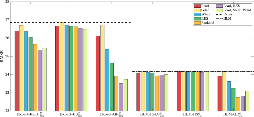
In Fig. 5, we report the RMSE for all proposed models that include the 201-quantile prediction of fundamental variables, and compare them to benchmarks that do not include any probabilistic inputs. We compare the accuracy of electricity price prediction across different base model structures, across different techniques for obtaining the probabilistic predictions of fundamental variables, and finally across different sets of these variables considered as probabilistic inputs. From the result presented in Fig. 5 we can draw some important conclusions:
-
•
In general, incorporating probabilistic inputs into the model improves the accuracy of electricity price forecasting. This is true for both base models with higher improvement for the Expert model (up to 13.3%; see Table I in Appendix).
-
•
As expected, the parameter-rich (HLM) based models outperformed their Expert model based counterparts. However, some Expert base models with probabilistic inputs (e.g., Expert-QR) outperformHLM based benchmark in term of accuracy.
-
•
Although any technique for obtaining probabilistic forecasts of the fundamental variables provides accuracy gains, by far the most accurate forecasts are obtained with probabilistic inputs calculated with QR. This indicates that the quality of the probabilistic forecast has a significant impact on the accuracy of the final electricity price forecasts.
-
•
For all considered cases, the best performing models include probabilistic information on all three considered fundamental variables ( {ResLoad}, {Load, RES} or {Load, Solar, Wind}). In particular, the best performing model is HML-QR, which reduces the RMSE by 16.6% and 6.1% compared to the Expert and HLM benchmarks, respectively.
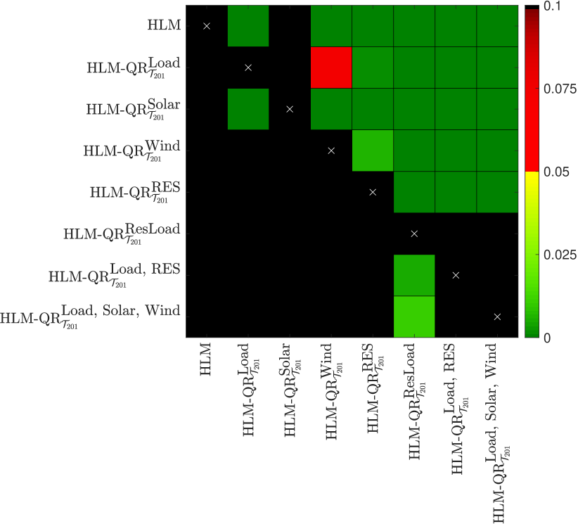
To formally confirm the significance of the difference between using different sets of fundamental variables included in the model in the form of probabilistic inputs in Fig. 6, we present the results of the CPA test for the HLM benchmark and all HLM-QR models.
As can be seen in Fig. 6, the HLM-QR models significantly outperform all other considered models. Overall, the three best models that significantly outperform other competitors include information about all three load, solar and wind (aggregated or not). On the other hand, the benchmark model without probabilistic inputs never outperforms any other model, while it performs significantly worse in 6 out of 7 cases, highlighting that including probabilistic inputs is beneficial in terms of forecast accuracy.
IV-B Comparison of different number of quantiles
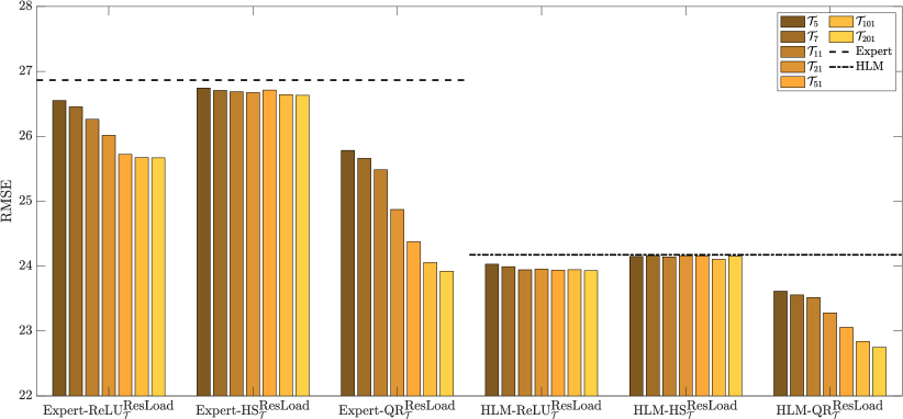
In Fig. 7 we present the similar comparison as in Fig. 5. However, this time we consider solely models including ResLoad and compare the forecast accuracy depending on number of considered probability levels. Note that even though we only present the results for models consisting ResLoad, the performance of other sets of variables are very similar (see Table I in Appendix).
Based on the results presented in Fig. 7, it can be seen that in general, the denser the grid of probability levels, the more accurate the predictions can be obtained. In particular, within the class of expert models, the best performing model is Expert-QR, while its HLM-based equivalent is the best performing model within the class of parameter-rich models.
IV-C Performance improvement analysis
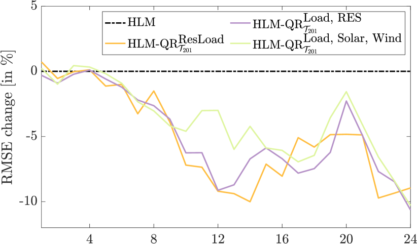
To analyze the performance of our newly proposed approach, in Fig. 8 we present the RMSE percentage improvement for different hours within a day. In Fig. 8 we compare the performance of three top performing models (HLM-QR, HLM-QR, HLM-QR) against the HLM benchmark. The percentage improvement for hour is defined as
| (10) |
where is the root mean square error for hour obtained with model .
As can be seen in Fig. 8, all three considered models outperform the benchmark for the majority of hours. Although the results of the models with different sets of probabilistic inputs are different, the overall trend remains the same. The improvement is smaller for the early morning hours (1-6), but increases to roughly 10% for the midday and late evening hours (22-24).
IV-D Selection and impact of probabilistic inputs
To answer the question of what is the most important factor in our approach that leads to a significant improvement in accuracy, we can further analyze how often each variable was selected in the final model and how given variables affect the prediction.
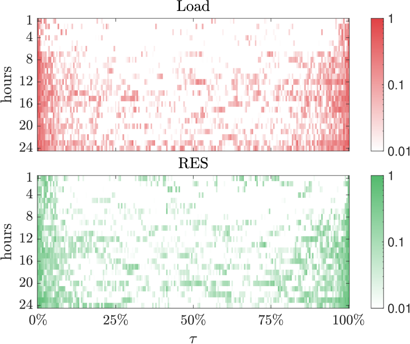
In Fig. 9 we show how often a given quantile prediction of load and RES was selected in the final model (corresponding value was different from 0). The results are presented for the HLM-QR model. The darker the color in Fig. 9, the more often the quantile prediction was selected as important by the LASSO regularization at the given probability level. It can be seen that by far the darkest places are on the left and right side of both plots, indicating that the extreme quantiles are selected much more often than the center of the distribution. Another interesting observation is that the probabilistic inputs are generally selected more frequently in the afternoon and evening hours and very rarely in the morning hours.
To analyze the impact of the probabilistic inputs on the forecast accuracy, in Fig. 10 we report the average impact of a given group of variables on the price forecast obtained with the HLM-QR model. First, in the left panel of Fig. 10 we plot the impact of 5 general groups of variables:
-
•
Autoregressive part consisting of 50 variables related to historical electricity prices ( to in Eq.(6)),
-
•
Load, which includes 48 variables related to the day-ahead load point forecasts ( to in equation (6)) plus 199 quantile load forecasts.
-
•
RES which includes 96 variables related to day-ahead point forecasts of solar and wind generation ( to in Eq. (6)) plus 199 quantile forecasts of RES
-
•
Commodities, including 4 variables ( to in equation (6))
-
•
Intercept, including 7 dummy variables ( to in eq. (6)) and intercept.
The middle and right panels in Fig. 10 show the impact of different parts of the distribution of predicted load and RES. The lower and upper tails are each represented by 21 quantile predictions (ranging from to 10% and from 90% to , respectively), while the middle of the distribution consists of 159 variables associated with quantile predictions with probability levels ranging from 10.5% to 74.5%.
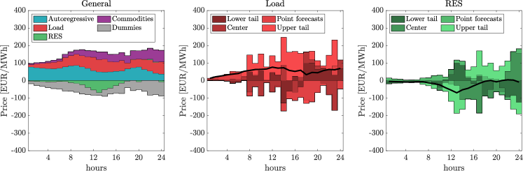
Based on Fig. 10 it can be seen that the proposed model exhibits stronger autoregressive behavior at the beginning of the day and weaker autoregressive behavior toward the end of the day, allowing for a greater influence of fundamental factors such as fuel prices. This is consistent with the current literature [35, 10]. However, the influence of RES seems to be significantly reduced, as it is mainly active in the middle of the day (probably related to solar generation).
For the middle and right plots in Fig. 10, it is evident that the impact is minimal during the early morning hours. This is likely due to the dominance of autoregressive information, with fundamental factors providing limited additional insight. Throughout the distribution – left tail, right tail, and center – each component is shown to be relevant, but their relative importance changes over time in a non-trivial manner.
V Conclusions
In this study, we propose and evaluate models that incorporate probabilistic forecasts of load and renewable energy sources (RES) into electricity price forecasts. Using automatic variable selection techniques such as LASSO, the models can include a large number of explanatory variables, including quantile forecasts for fundamental inputs.
Our analysis shows that the integration of probabilistic inputs significantly improves forecast accuracy. Among the parameter-rich HLM-based models and their expert counterparts, the HLM-QR model performs best, reducing the RMSE by 16.5 % and 6.1% over the expert and HLM benchmarks, respectively.
In addition, the quality of the probabilistic predictions of the fundamental variables strongly affects the performance of the models, with quantile regression (QR) being the most successful. Analysis of quantile inclusion revealed that denser grids of quantiles consistently improved forecast accuracy, highlighting the importance of research in probabilistic forecasting of load and RES generation. Particularly, in wind and solar power forecasting, probabilistic forecasts are hardly used in practice for decision making. Even if probabilistic forecasts are utilized, this is usually only for very limited quantiles, e.g. 10%, 50% and 90% while a denser information set would be significantly better.
The results indicate that the performance improvements were not uniform across all hours: while the gains were relatively small in the early hours of the day, they were very substantial in the late hours of the day. This variability is consistent with the observation that probabilistic inputs are selected more frequently in the afternoon and evening hours, particularly extreme quantiles, which are more relevant at these times.
References
- [1] J. Lange and M. Kaltschmitt, “Probabilistic day-ahead forecast of available thermal storage capacities in residential households,” Applied Energy, vol. 306, p. 117957, 2022.
- [2] M. G. Pollitt and C. K. Chyong, “Modelling net zero and sector coupling: Lessons for European policy makers,” Economics of Energy and Environmental Policy, vol. 10, no. 2, pp. 25–40, 2021.
- [3] A. Gianfreda, L. Parisio, and M. Pelagatti, “The impact of RES in the Italian day-ahead and balancing markets,” Energy Journal, vol. 37, pp. 161–184, 2016.
- [4] T. Hong, P. Pinson, Y. Wang, R. Weron, D. Yang, and H. Zareipour, “Energy forecasting: A review and outlook,” IEEE Open Access Journal of Power and Energy, vol. 7, pp. 376–388, 2020.
- [5] J. Lago, G. Marcjasz, B. De Schutter, and R. Weron, “Forecasting day-ahead electricity prices: A review of state-of-the-art algorithms, best practices and an open-access benchmark,” Applied Energy, vol. 293, p. 116983, 2021.
- [6] R. Huisman and C. Stet, “The dependence of quantile power prices on supply from renewables,” Energy Economics, vol. 105, p. 105685, 2022.
- [7] S. Kulakov and F. Ziel, “The impact of renewable energy forecasts on intraday electricity prices,” Economics of Energy and Environmental Policy, vol. 10, pp. 79–104, 2021.
- [8] R. Weron, “Electricity price forecasting: A review of the state-of-the-art with a look into the future,” International Journal of Forecasting, vol. 30, no. 4, pp. 1030–1081, 2014.
- [9] S. Kolb, M. Dillig, T. Plankenbühler, and J. Karl, “The impact of renewables on electricity prices in germany-an update for the years 2014–2018,” Renewable and Sustainable Energy Reviews, vol. 134, p. 110307, 2020.
- [10] P. Ghelasi and F. Ziel, “Far beyond day-ahead with econometric models for electricity price forecasting,” arXiv preprint arXiv:2406.00326, 2024.
- [11] R. Tibshirani, “Regression shrinkage and selection via the lasso,” Journal of the Royal Statistical Society B, vol. 58, pp. 267–288, 1996.
- [12] M. Narajewski and F. Ziel, “Econometric modelling and forecasting of intraday electricity prices,” Journal of Commodity Markets, vol. 19, p. 100107, 2020.
- [13] R. Giacomini and H. White, “Tests of conditional predictive ability,” Econometrica, vol. 74, no. 6, pp. 1545–1578, 2006.
- [14] A. Lipiecki, B. Uniejewski, and R. Weron, “Postprocessing of point predictions for probabilistic forecasting of day-ahead electricity prices: The benefits of using isotonic distributional regression,” Energy Economics, vol. 139, p. 107934, 2024.
- [15] B. Liu, J. Nowotarski, T. Hong, and R. Weron, “Probabilistic load forecasting via Quantile Regression Averaging on sister forecasts,” IEEE Transactions on Smart Grid, vol. 8, pp. 730–737, 2017.
- [16] Y. Wang, N. Zhang, Y. Tan, T. Hong, D. Kirschen, and C. Kang, “Combining probabilistic load forecasts,” IEEE Transactions on Smart Grid, vol. 10, no. 4, pp. 3664–3674, 2019.
- [17] B. Uniejewski and R. Weron, “Regularized quantile regression averaging for probabilistic electricity price forecasting,” Energy Economics, vol. 95, p. 105121, 2021.
- [18] J. Berrisch and F. Ziel, “CRPS learning,” Journal of Econometrics, 2023, dOI: 10.1016/j.jeconom.2021.11.008.
- [19] D. Yang, G. Yang, and B. Liu, “Combining quantiles of calibrated solar forecasts from ensemble numerical weather prediction,” Renewable Energy, vol. 215, p. 118993, 2023.
- [20] C. Cornell, N. T. Dinh, and S. A. Pourmousavi, “A probabilistic forecast methodology for volatile electricity prices in the Australian National Electricity Market,” International Journal of Forecasting,, 2024.
- [21] R. W. Koenker, Quantile Regression. Cambridge University Press, 2005.
- [22] V. Chernozhukov, I. Fernandez-Val, and A. Galichon, “Quantile and probability curves without crossing,” Econometrica, vol. 73, no. 3, pp. 1093–1125, 2010.
- [23] K. Maciejowska and J. Nowotarski, “A hybrid model for GEFCom2014 probabilistic electricity price forecasting,” International Journal of Forecasting, vol. 32, no. 3, pp. 1051–1056, 2016.
- [24] A. Billé, A. Gianfreda, F. Del Grosso, and F. Ravazzolo, “Forecasting electricity prices with expert, linear, and nonlinear models,” International Journal of Forecasting, vol. 39, no. 2, pp. 570–586, 2023.
- [25] P. Gaillard, Y. Goude, and R. Nedellec, “Additive models and robust aggregation for GEFCom2014 probabilistic electric load and electricity price forecasting,” International Journal of Forecasting, vol. 32, no. 3, pp. 1038–1050, 2016.
- [26] K. Hubicka, G. Marcjasz, and R. Weron, “A note on averaging day-ahead electricity price forecasts across calibration windows,” IEEE Transactions on Sustainable Energy, vol. 10, no. 1, pp. 321–323, 2019.
- [27] B. Uniejewski, “Regularization for electricity price forecasting,” Operations Research and Decisions, vol. 34, no. 3, pp. 267–286, 2024.
- [28] F. Ziel and R. Weron, “Day-ahead electricity price forecasting with high-dimensional structures: Univariate vs. multivariate modeling frameworks,” Energy Economics, vol. 70, pp. 396–420, 2018.
- [29] B. Uniejewski, J. Nowotarski, and R. Weron, “Automated variable selection and shrinkage for day-ahead electricity price forecasting,” Energies, vol. 9, p. 621, 2016.
- [30] F. Ziel, “Forecasting electricity spot prices using lasso: On capturing the autoregressive intraday structure,” IEEE Transactions on Power Systems, vol. 31, no. 6, pp. 4977–4987, 2016.
- [31] J. Lago, F. De Ridder, and B. De Schutter, “Forecasting spot electricity prices: Deep learning approaches and empirical comparison of traditional algorithms,” Applied Energy, vol. 221, pp. 386–405, 2018.
- [32] K. Maciejowska, B. Uniejewski, and R. Weron, “Forecasting electricity prices,” Oxford Research Encyclopedia of Economics and Finance, 2023, Forthcoming. DOI (arXiv): 10.48550/arXiv.2204.11735.
- [33] A. Wagner, E. Ramentol, F. Schirra, and H. Michaeli, “Short- and long-term forecasting of electricity prices using embedding of calendar information in neural networks,” Journal of Commodity Markets, vol. 28, p. 100246, 2022.
- [34] B. Uniejewski, R. Weron, and F. Ziel, “Variance stabilizing transformations for electricity spot price forecasting,” IEEE Transactions on Power Systems, vol. 33, pp. 2219–2229, 2018.
- [35] R. Sgarlato and F. Ziel, “The role of weather predictions in electricity price forecasting beyond the day-ahead horizon,” IEEE Transactions on Power Systems, vol. 38, no. 3, pp. 2500–2511, 2023.
| – | – | 26.86 | ||||||||||||||
|
RMSE |
%chng |
RMSE |
%chng |
RMSE |
%chng |
RMSE |
%chng |
RMSE |
%chng |
RMSE |
%chng |
RMSE |
%chng |
|||
| Load | 26.78 | -0.3 | 26.84 | -0.1 | 26.80 | -0.3 | 26.69 | -0.7 | 26.52 | -1.3 | 26.43 | -1.6 | 26.40 | -1.8 | ||
| Solar | 26.80 | -0.2 | 26.81 | -0.2 | 26.81 | -0.2 | 26.74 | -0.5 | 26.71 | -0.6 | 26.68 | -0.7 | 26.71 | -0.6 | ||
| Wind | 26.86 | 0.0 | 26.90 | 0.1 | 26.83 | -0.1 | 26.72 | -0.6 | 26.58 | -1.1 | 26.43 | -1.6 | 26.37 | -1.9 | ||
| RES | 26.73 | -0.5 | 26.63 | -0.9 | 26.59 | -1.0 | 26.41 | -1.7 | 26.20 | -2.5 | 26.10 | -2.9 | 26.06 | -3.1 | ||
| ResLoad | 26.55 | -1.2 | 26.45 | -1.5 | 26.26 | -2.3 | 26.02 | -3.2 | 25.72 | -4.4 | 25.67 | -4.5 | 25.67 | -4.6 | ||
| Load, RES | 26.62 | -0.9 | 26.62 | -0.9 | 26.54 | -1.2 | 26.25 | -2.3 | 25.78 | -4.1 | 25.52 | -5.1 | 25.32 | -5.9 | ||
|
ReLU |
Load, Solar, Wind | 26.73 | -0.5 | 26.80 | -0.2 | 26.69 | -0.6 | 26.34 | -2.0 | 25.99 | -3.3 | 25.63 | -4.7 | 25.46 | -5.4 | |
| Load | 26.66 | -0.7 | 26.67 | -0.7 | 26.66 | -0.8 | 26.63 | -0.9 | 26.59 | -1.0 | 26.61 | -0.9 | 26.67 | -0.7 | ||
| Solar | 26.89 | 0.1 | 26.87 | 0.0 | 26.89 | 0.1 | 26.89 | 0.1 | 26.89 | 0.1 | 26.87 | 0.0 | 26.87 | 0.0 | ||
| Wind | 26.83 | -0.1 | 26.83 | -0.1 | 26.83 | -0.1 | 26.83 | -0.1 | 26.76 | -0.4 | 26.74 | -0.5 | 26.72 | -0.5 | ||
| RES | 26.81 | -0.2 | 26.80 | -0.2 | 26.76 | -0.4 | 26.75 | -0.4 | 26.73 | -0.5 | 26.69 | -0.7 | 26.66 | -0.8 | ||
| ResLoad | 26.74 | -0.5 | 26.70 | -0.6 | 26.69 | -0.7 | 26.67 | -0.7 | 26.71 | -0.6 | 26.64 | -0.8 | 26.63 | -0.9 | ||
| Load, RES | 26.64 | -0.9 | 26.63 | -0.9 | 26.64 | -0.9 | 26.60 | -1.0 | 26.57 | -1.1 | 26.55 | -1.2 | 26.55 | -1.2 | ||
|
HS |
Load, Solar, Wind | 26.70 | -0.6 | 26.69 | -0.7 | 26.67 | -0.7 | 26.66 | -0.8 | 26.55 | -1.2 | 26.55 | -1.2 | 26.50 | -1.4 | |
| Load | 26.51 | -1.3 | 26.44 | -1.6 | 26.43 | -1.6 | 26.25 | -2.3 | 26.16 | -2.6 | 26.11 | -2.9 | 26.12 | -2.8 | ||
| Solar | 26.83 | -0.1 | 26.82 | -0.2 | 26.78 | -0.3 | 26.73 | -0.5 | 26.72 | -0.5 | 26.74 | -0.5 | 26.73 | -0.5 | ||
| Wind | 26.29 | -2.2 | 26.22 | -2.4 | 26.07 | -3.0 | 25.93 | -3.6 | 25.67 | -4.5 | 25.55 | -5.0 | 25.39 | -5.6 | ||
| RES | 25.75 | -4.2 | 25.65 | -4.6 | 25.51 | -5.2 | 25.23 | -6.3 | 24.89 | -7.6 | 24.80 | -8.0 | 24.63 | -8.7 | ||
| ResLoad | 25.78 | -4.1 | 25.66 | -4.6 | 25.48 | -5.3 | 24.87 | -7.7 | 24.38 | -9.7 | 24.05 | -11.1 | 23.92 | -11.6 | ||
| Load, RES | 25.23 | -6.3 | 25.06 | -7.0 | 24.85 | -7.8 | 24.31 | -10.0 | 23.88 | -11.8 | 23.74 | -12.4 | 23.52 | -13.3 | ||
|
Expert |
QR |
Load, Solar, Wind | 25.44 | -5.4 | 25.27 | -6.1 | 25.09 | -6.8 | 24.59 | -8.9 | 24.21 | -10.4 | 23.92 | -11.6 | 23.75 | -12.3 |
| – | – | 24.17 | ||||||||||||||
|
RMSE |
%chng |
RMSE |
%chng |
RMSE |
%chng |
RMSE |
%chng |
RMSE |
%chng |
RMSE |
%chng |
RMSE |
%chng |
|||
| Load | 24.13 | -0.2 | 24.17 | 0.0 | 24.17 | 0.0 | 24.13 | -0.2 | 24.13 | -0.2 | 24.10 | -0.3 | 24.08 | -0.4 | ||
| Solar | 24.17 | 0.0 | 24.17 | 0.0 | 24.15 | -0.1 | 24.15 | -0.1 | 24.17 | 0.0 | 24.15 | -0.1 | 24.15 | -0.1 | ||
| Wind | 24.20 | 0.1 | 24.21 | 0.1 | 24.18 | 0.0 | 24.17 | 0.0 | 24.19 | 0.0 | 24.16 | 0.0 | 24.13 | -0.2 | ||
| RES | 24.13 | -0.2 | 24.09 | -0.3 | 24.08 | -0.4 | 24.07 | -0.4 | 24.06 | -0.5 | 24.07 | -0.4 | 24.08 | -0.4 | ||
| ResLoad | 24.03 | -0.6 | 23.99 | -0.8 | 23.94 | -1.0 | 23.95 | -0.9 | 23.94 | -1.0 | 23.95 | -1.0 | 23.93 | -1.0 | ||
| Load, RES | 24.08 | -0.4 | 24.07 | -0.5 | 24.04 | -0.6 | 23.99 | -0.8 | 24.04 | -0.5 | 23.99 | -0.8 | 23.98 | -0.8 | ||
|
ReLU |
Load, Solar, Wind | 24.14 | -0.1 | 24.15 | -0.1 | 24.10 | -0.3 | 24.09 | -0.4 | 24.04 | -0.6 | 24.00 | -0.7 | 24.00 | -0.7 | |
| Load | 24.14 | -0.1 | 24.18 | 0.0 | 24.17 | 0.0 | 24.16 | -0.1 | 24.16 | -0.1 | 24.16 | 0.0 | 24.17 | 0.0 | ||
| Solar | 24.20 | 0.1 | 24.22 | 0.2 | 24.18 | 0.0 | 24.17 | 0.0 | 24.21 | 0.1 | 24.18 | 0.0 | 24.17 | 0.0 | ||
| Wind | 24.19 | 0.1 | 24.19 | 0.1 | 24.18 | 0.0 | 24.19 | 0.1 | 24.17 | 0.0 | 24.17 | 0.0 | 24.15 | -0.1 | ||
| RES | 24.17 | 0.0 | 24.16 | -0.1 | 24.17 | 0.0 | 24.16 | -0.1 | 24.16 | -0.1 | 24.15 | -0.1 | 24.16 | -0.1 | ||
| ResLoad | 24.15 | -0.1 | 24.16 | 0.0 | 24.14 | -0.1 | 24.16 | -0.1 | 24.16 | -0.1 | 24.11 | -0.3 | 24.15 | -0.1 | ||
| Load, RES | 24.13 | -0.2 | 24.14 | -0.1 | 24.14 | -0.2 | 24.14 | -0.1 | 24.15 | -0.1 | 24.13 | -0.2 | 24.13 | -0.2 | ||
|
HS |
Load, Solar, Wind | 24.16 | 0.0 | 24.14 | -0.1 | 24.17 | 0.0 | 24.17 | 0.0 | 24.13 | -0.2 | 24.13 | -0.2 | 24.14 | -0.1 | |
| Load | 23.97 | -0.8 | 23.98 | -0.8 | 23.98 | -0.8 | 23.94 | -1.0 | 23.93 | -1.0 | 23.94 | -1.0 | 23.92 | -1.1 | ||
| Solar | 24.18 | 0.0 | 24.17 | 0.0 | 24.18 | 0.0 | 24.16 | 0.0 | 24.17 | 0.0 | 24.17 | 0.0 | 24.15 | -0.1 | ||
| Wind | 23.94 | -1.0 | 23.95 | -0.9 | 23.93 | -1.0 | 23.87 | -1.3 | 23.76 | -1.7 | 23.72 | -1.9 | 23.62 | -2.3 | ||
| RES | 23.63 | -2.3 | 23.66 | -2.1 | 23.66 | -2.1 | 23.59 | -2.4 | 23.42 | -3.2 | 23.38 | -3.4 | 23.26 | -3.9 | ||
| ResLoad | 23.61 | -2.4 | 23.56 | -2.6 | 23.52 | -2.8 | 23.28 | -3.8 | 23.06 | -4.7 | 22.84 | -5.7 | 22.75 | -6.1 | ||
| Load, RES | 23.39 | -3.3 | 23.40 | -3.3 | 23.40 | -3.2 | 23.22 | -4.0 | 23.08 | -4.6 | 22.96 | -5.2 | 22.83 | -5.7 | ||
|
HLM |
QR |
Load, Solar, Wind | 23.68 | -2.1 | 23.68 | -2.1 | 23.63 | -2.3 | 23.52 | -2.7 | 23.29 | -3.7 | 23.20 | -4.1 | 23.10 | -4.5 |