Precoding Design for Limited-Feedback MISO Systems via Character-Polynomial Codes

Abstract

We consider the problem of Multiple-Input Single-Output (MISO) communication with limited feedback, where the transmitter relies on a limited number of bits associated with the channel state information (CSI), available at the receiver (CSIR) but not at the transmitter (no CSIT), sent via the feedback link. We demonstrate how character-polynomial (CP) codes, a class of analog subspace codes (also, referred to as Grassmann codes) can be used for the corresponding quantization problem in the Grassmann space. The proposed CP codebook-based precoding design allows for a smooth trade-off between the number of feedback bits and the beamforming gain, by simply adjusting the rate of the underlying CP code. We present a theoretical upper bound on the mean squared quantization error of the CP codebook, and utilize it to upper bound the resulting distortion as the normalized gap between the CP codebook beamforming gain and the baseline equal gain transmission (EGT) with perfect CSIT. We further show that the distortion vanishes asymptotically. The results are also confirmed via simulations for different types of fading models in the MISO system and various parameters.

I Introduction

Multiple-input multiple-output (MIMO) antenna systems continue to be a critical part of the physical layer design of the next generation, 6G and beyond, wireless networks  [1]. MIMO systems can exploit channel state information (CSI) at the transmitter for precoding, rate adaptation, and multiuser MIMO transmission to improve spectral efficiency [2]. The most common means for obtaining knowledge about the CSI at the transmitter is known as limited feedback, where CSI is quantized and sent to the transmitter via a finite rate feedback channel  [3, 4, 5]. The problem of limited feedback for precoding in MIMO systems is sometimes known as Grassmannian feedback, due to the mathematical connections between quantizing the dominate subspaces of a MIMO channel and packing problems in the Grassmannian space [6]. Relevant prior works include bounds for Grassmannian coding [7, 8, 9], codebook designs [10, 11, 12], structured codebooks [13, 14, 15], codebooks that exploit spatial correlation [16], and codebooks that exploit time variation [17].

The earliest work on codebook design for limited feedback MIMO systems made connections between the limited feedback problem and subspace packings on the Grassmann manifold through bounds on the mutual information as a function of the minimum subspace distance [6]. For the most part, the resulting codebooks were either related to known designs at the time or were numerically designed for Grassmannian packings [6, 12]. Another line of work has considered structured codebooks that may be suboptimal but easier to store or search including Kerdock codebooks [18, 19]. A different line of work considers the problem of designing large codebooks with a structure to facilitate encoding to avoid a brute force search [20, 21, 22]. Prior work has not considered connections between the related problem of Grassmannian coding [6] and general methodologies for designing large codebooks with desirable structural constraints such as having entries with equal gains.

In this paper, we develop limited feedback codebooks that can be stored easily and searched in polynomial time. More specifically, we use character-polynomial (CP) codes, a class of analog subspace codes (also, referred to as Grassmann codes) recently introduced in [15] for the beamforming quantization problem. CP codes provide a new solution for Grassmannian line packing problem, and have been also extended to provide packings for higher-dimensional subspaces [23]. The CP codebook vectors have equal magnitudes across their entries, which is an advantageous structural property that preserves per-antenna power constraints. We characterize and bound the mean squared quantization error and the distortion of the resulting scheme for quantizing the optimal beamforming vector. The distortion is measured with respect to the performance of equal gain transmission (EGT) with perfect CSIT [24]. The bounds are valid for memoryless channels experiencing i.i.d. complex-valued fading regardless of the fading distribution. Simulations are provided for MISO systems with Rayleigh and Rician fading distributions confirming these theoretical findings. We also compare the CP codebook with the PSK codebook of [20] as the most relevant prior work, where the advantages of our scheme is twofold. The CP code rate offers a new knob to tune which allows a more flexible trade off between the beamforming gain and the number of feedback bits. Furthermore, the beamforming gain of CP codebook is improved, compared to the PSK codebook across different numbers of feedback bits and by up to $\sim 1$dB.

II Preliminaries and Related Work

II-A Notation Convention

We use bold capital letters (e.g. $\mathbf{X}$) to represent matrices, and bold small letters (e.g. $\mathbf{x}$) for vectors. We also reserve $|\cdot|$ for the absolute value of a complex number and use $\left\|{\,\cdot\,}\right\|$ for the $L^{2}$-norm of a vector.

II-B Chordal Distance and Subspace Codes

Given an ambient vector space $W$, ${\mathcal{P}}(W)$ and ${\mathcal{P}}_{m}(W)$ respectively denote the set of all of its subspaces and the set of all of its $m$-dimensional subspaces. ${\mathcal{P}}_{m}({\mathbb{C}}^{n})$ is referred to as a Grassmannian space and is denoted $G_{m,n}({\mathbb{C}})$. Any $U\in G_{m,n}({\mathbb{C}})$ is equipped with the natural inner product $\langle{\bf u},{\bf v}\rangle:={{\bf u}}^{\dagger}{\bf v}$ for ${\bf u},{\bf v}\in U$.

Definition 1.

Let $U,V\in G_{m,n}({\mathbb{C}})$ . Let ${\bf u}_{i}\in U$ and ${\bf v}_{i}\in V$, for $i\in[m]$, be vectors such that $|\langle{\bf u}_{i},{\bf v}_{i}\rangle|$ is maximal, subject to the condition that they form orthonormal bases for $U$ and $V$, respectively. Then the $i$-th principal angle $\theta_{i}$ between $U$ and $V$ is defined as $\theta_{i}=\arccos|\langle{\bf u}_{i},{\bf v}_{i}\rangle|$. Then the chordal distance [10] between $U$ and $V$ is

$$d_{{\rm C}}(U,V):=\sqrt{\sum_{i=1}^{m}\sin^{2}\theta_{i}}$$ (1)

An analog subspace code is a collection ${\mathcal{C}}\subseteq{\mathcal{P}}({\mathbb{C}}^{n})$ of subspaces. When the dimension of all subspace codewords is the same, the code is also referred to as a Grassmann code.

II-C CP Codes

Let ${\mathbb{F}}_{q}$ be a finite field of size $q$ and characteristic $p$. Let

$${\mathcal{F}}(k,q) :=\{f\in{\mathbb{F}}_{q}[X]:\deg(f)\leq k\}$$ (2)

for $k<q$ denote the set of all polynomials of degree at most $k$ over ${\mathbb{F}}_{q}$. This serves as the message space for classical Reed-Solomon (RS) codes. The elements of ${\mathcal{F}}(k,q)$ are called message polynomials, whose coefficients represent the message symbols. We also define ${\mathcal{F}}_{p}(k,q)$ to be the set of all $f(X)=\sum_{j}f_{j}X^{j}\in{\mathcal{F}}(k,q)$ with $f_{jp}=0$ for all integers $j\geq 0$, and ${\mathcal{F}}_{p}(k,q)^{\prime}:=\{f(X)/X:f\in{\mathcal{F}}_{p}(k,q)\}$.

Definition 2 (CP Code [15, Definition 6]).

Fix $k\leq n<q$, a non-trivial character $\chi$ of ${\mathbb{F}}_{q}$, and units $\alpha_{1},\dots,\alpha_{n}\in{\mathbb{F}}_{q}^{\times}:={\mathbb{F}}_{q}\setminus\{0\}$. Then the encoding of $f\in{\mathcal{F}}_{p}(k,q)$ in $\operatorname{CP}:=\operatorname{CP}_{n}({\mathcal{F}}_{p}(k,q),\chi)\subseteq G_{1,n}({\mathbb{C}})$ is given by

$$\operatorname{CP}(f) :=(\chi(f(\alpha_{1})),\dots,\chi(f(\alpha_{n}))),$$ (3)

where we identify $\operatorname{CP}(f)$ with the one-dimensional subspace $\langle\operatorname{CP}(f)\rangle$.

$\operatorname{CP}_{n}({\mathcal{F}}_{p}(k,q),\chi)$ is essentially the concatenation of a subcode of a generalized Reed–Solomon (GRS) code, where a certain subset of the coefficients of the message polynomial is set to zeros, followed by the character mapping $\chi$ to the complex unit circle. Roughly speaking, this can be regarded as a certain GRS-coded modulation.

Given $k\leq n\leq q$, distinct $\alpha_{1},\dots,\alpha_{n}\in{\mathbb{F}}_{q}$ and not necessarily distinct $\beta_{1},\dots,\beta_{n}\in{\mathbb{F}}_{q}^{\times}$, the encoding of $f\in{\mathcal{F}}(k-1,q)$ in $\operatorname{GRS}:=\operatorname{GRS}_{n}({\mathcal{F}}(k-1,q))$ is given by

$$\operatorname{GRS}(f) :=(\beta_{1}f(\alpha_{1}),\dots,\beta_{n}f(\alpha_{n})).$$ (4)

Let $\beta_{i}=\alpha_{i}$ for $i\in\{1,\dots,n\}$. Using the notation introduced above, $\operatorname{CP}_{n}({\mathcal{F}}_{p}(k,q),\chi)$ prior to concatenation by $\chi$ can be expressed as $\operatorname{GRS}_{n}({\mathcal{F}}_{p}(k,q)^{\prime})$. Therefore,

$$|\operatorname{CP}|=|{\mathcal{F}}_{p}(k,q)|=|{\mathcal{F}}_{p}(k,q)^{\prime}|=q^{k-\lfloor k/p\rfloor}.$$ (5)

See also [15, Theorem 9].

For the sake of simplicity, our primary focus will be on the case of prime fields, i.e., when $q=p$. In this case, observe that the dimension of $\operatorname{CP}_{n}({\mathcal{F}}_{p}(k,q),\chi)$, which is $k$ by (5), is equal to the dimension of $\operatorname{GRS}_{n}({\mathcal{F}}(k-1,q))$, where the message polynomials have degree at most $k-1$.

II-D Covering Radius and Mean Quantization Error

The covering radius of a block code ${\mathcal{C}}\subseteq{\mathbb{F}}^{n}$ is defined as

$$\rho_{{\rm H}}({\mathcal{C}}) :=\max_{{\bf y}\in{\mathbb{F}}^{n}}\min_{{\bf c}\in{\mathcal{C}}}d_{{\rm H}}({\bf y},{\bf c}),$$ (6)

where $d_{{\rm H}}$ is the Hamming distance. For instance, $\rho_{{\rm H}}(\operatorname{GRS})=n-k$ (see, e.g. [25]). The chordal covering radius of an analog subspace code ${\mathcal{C}}\subseteq{\mathcal{P}}({\mathbb{C}}^{n})$ may be analogously defined as

$$\rho_{{\rm C}}({\mathcal{C}}) :=\max_{U\in{\mathcal{P}}({\mathbb{C}}^{n})}\min_{V\in{\mathcal{C}}}d_{{\rm C}}(U,V),$$ (7)

where $d_{{\rm C}}(.,.)$ is the chordal distance defined in (1).

The covering radius can be thought of as the maximum error, in the sense of the underlying distance defined for the space, when using a code for the quantization of the space. Such a quantization is done by mapping any given element in the space to the closest codeword. Note that covering radius characterizes the worst-case scenario of the quantization process. However, in practice, given a certain distribution over the space, the average quantization error becomes more relevant. This is defined formally next.

Definition 3 (Mean Squared Quantization Error).

Let ${\mathcal{C}}\subseteq{\mathcal{P}}({\mathbb{C}}^{n})$ be an analog subspace code and ${\mathcal{D}}$ a distribution on ${\mathcal{P}}({\mathbb{C}}^{n})$. Then the mean squared quantization error of ${\mathcal{C}}$ over ${\mathcal{D}}$ is defined as

$$Q_{\rm e}({\mathcal{C}}) :=\operatorname*{\mathbb{E}}_{U\sim{\mathcal{D}}}\left[\min_{V\in{\mathcal{C}}}d_{{\rm C}}(U,V)^{2}\right],$$ (8)

where $d_{{\rm C}}(.,.)$ is the chordal distance defined in (1).

We see in the next section that this notion can capture the average beamforming gain. Note also that $Q_{\rm e}({\mathcal{C}})\leq\rho_{{\rm C}}({\mathcal{C}})^{2}$.

III System Model

We consider the MISO system in Figure 1, where the transmitter is equipped with $N_{T}$ transmit antennas and the receiver is assumed to have perfect CSIR enabling it to compute the optimal beamforming vector. Let the channel $\mathbf{h}\in\mathbb{C}^{1\times N_{T}}$ be a memoryless complex-valued fading channel with i.i.d. entries. With transmit beamforming and receive combining, let $x\in\mathbb{C}$ and $y\in\mathbb{C}$ denote the input and output of the system with

$$y=z^{*}\mathbf{h}\mathbf{f}x+{z^{*}}{n},$$ (9)

where $\mathbf{f}\in\mathbb{C}^{N_{T}\times 1}$ is the beamforming vector, ${z}$ is the combining unit complex scalar, and ${n}\in\mathbb{C}$ is a circularly symmetric complex Gaussian random variable with variance $N_{0}$. Keeping the design constraints in perspective, the norm of the beamforming vectors is set to unity, i.e. $\|\mathbf{f}\|=1.$ Then the overall gain $\Gamma(\mathbf{h})$, given the beamforming and combining is given by

$$\Gamma(\mathbf{h})=|{z}^{*}\mathbf{h}\mathbf{f}|^{2}.$$ (10)

Ideally, maximum ratio transmission (MRT) and maximum ratio combining (MRC) are employed to maximize the overall gain [26]. This is done by setting the combining and beamforming vectors to be the left and right singular vectors of the channel, respectively. For $N_{R}=1$, the MRT gain, denoted in short by $\Gamma_{\textup{MRT}}$, is equal to $\Gamma_{\textup{MRT}}(\mathbf{h})=\|\mathbf{h}\|^{2}$, when the combining unit complex scalar is of the form $z=\frac{\mathbf{hf}}{\|\mathbf{hf}\|}$.

Note that $\mathbf{h}$ is assumed to be only known at the receiver. Hence, only the receiver (and not the transmitter) can compute the optimal combining and beamforming vectors. The goal is to design a codebook $\mathcal{C}$ for the beamforming vectors, that the transmitter and receiver can agree upon prior to communication. =Then the receiver maps the optimal beamforming vector $\mathbf{f^{\rm opt}}=\gamma\frac{\mathbf{h}}{\|\mathbf{h}\|}$, where $\gamma$ is a unit complex number, to the closest (to be specified later) element of the codebook. The result of this can be conveyed back to the transmitter using $\lceil\log_{2}|\mathcal{C}|\rceil$ bits.

It is known that [6, 20], the beamforming gain of the codebook $\mathcal{C}$ relates to $\Gamma_{\textup{MRT}}(\mathbf{h})$ as follows:

$$\frac{\Gamma_{\mathcal{C}}(\mathbf{h})}{\Gamma_{\textup{MRT}}(\mathbf{h})}=\cos^{2}\theta(\mathbf{f^{\rm opt}},\mathbf{f^{\rm opt}_{\mathcal{C}}}),$$ (11)

where $\mathbf{f^{\rm opt}_{\mathcal{C}}}\in\mathcal{C}$ maximizes the beamforming gain, and $\theta(.,.)$ denotes the principal angle.

In other words, the problem of searching for the optimal beamforming vector in $\mathcal{C}$ is equivalent to solving the following:

$$\mathbf{f^{\rm opt}_{\mathcal{C}}}=\operatorname*{arg\,max}_{\mathbf{f}\in\mathcal{C}}\cos^{2}\theta(\mathbf{f^{\rm opt}},\mathbf{f}).$$ (12)

Remark 1.

The maximization in (12) (equivalent to maximizing the beamforming gain in (11)) is also equivalent to minimization of the chordal distance between $\mathbf{f}^{\rm opt}$ and $\mathbf{f}$. This is established in [6] which serves as the foundation for relating the problem of optimal beamforming design and packing lines in the Grassmannian space. Then, given the codebook $\mathcal{C}$ of all possible beamforming vectors $\mathbf{f}$, the problem to solve at the receiver is to search for the codeword that is closest, in chordal distance, to $\mathbf{f}^{\rm opt}$.

Remark 2.

In light of Remark 1, note also that

$$d_{{\rm C}}(\mathbf{f^{\rm opt}},\mathbf{f^{\rm opt}_{\mathcal{C}}})^{2}=1-\cos^{2}\theta(\mathbf{f^{\rm opt}},\mathbf{f^{\rm opt}_{\mathcal{C}}}).$$ (13)

Hence, given a certain distribution on $\mathbf{h}$, minimizing the mean squared quantization error, as defined in Definition 3, is also equivalent to maximizing the average beamforming gain. Generally speaking, the smaller the average quantization error is for a codebook $\mathcal{C}$, the larger its average beamforming gain becomes.

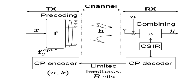
Figure 1: Downlink beamforming quantization design with limited feedback using CP codebook

An alternative baseline for the beamforming gain is EGT [24], where all the coordinates of the EGT beamforming vector have equal amplitude (the equal gain condition). This is appealing from a hardware implementation perspective as it simplifies the amplifier design for the antenna beamforming system. In this case, the optimization of the beamforming gain is only over the $N_{T}$ phases of the beamforming vector. The EGT gain with optimal EGT vector is given by [24]

$$\Gamma_{\textup{EGT}}(\mathbf{h}) =\frac{\|\mathbf{h}\|_{1}^{2}}{N_{T}}.$$ (14)

Note that, naturally, $\Gamma_{\textup{EGT}}(\mathbf{h})\leq\Gamma_{\textup{MRT}}(\mathbf{h})$.

The CP codebook that we consider in this paper satisfies the equal gain condition. Hence, its beamforming gain will be compared with the EGT beamforming gain both analytically as well as in simulations.

IV CP Codebook Beamforming

IV-A Construction, Feedback Design, and Beamforming Search

Consider a $\operatorname{CP}$ codebook $\mathcal{C}$ over a prime field ${\mathbb{F}}_{p}$, as defined in Definition 2. More specifically, ${\mathcal{C}}$ consists of codewords $\operatorname{CP}(f)$ for $f\in{\mathcal{F}}_{p}(k,p)$. Then the size of the codebook for a given dimension $k$ is $|\mathcal{C}|=p^{k}$. The parameter $n$ of the CP codebook is set as $n=N_{T}$.

The number $B$ of feedback bits from the receiver to the transmitter, to specify which beamforming vector from the CP codebook to use, is given by:

$$B =\lceil\log_{2}|\mathcal{C}|\rceil=\lceil\log_{2}(p^{k})\rceil=\lceil k\log_{2}p\rceil,$$

which scales linearly with the dimension $k$ of the code and logarithmically with the number of antennas as $n\leq p-1$ (one can pick the smallest $p\geq n+1$ for the codebook design).

Note that the CP codebook can be saved efficiently at the receiver by simply storing the parameters $\alpha_{i}$’s (with $n\log_{2}p$ bits) together with the character function $\chi$ (with $\log_{2}n$ bits). The complexities, for both storage and encoding, are essentially the same as those of classical Reed-Solomn codes that are widely used in practice [27].

As discussed in Section III for a general codebook $\mathcal{C}$, the problem of searching for the optimal beamforming vector $\mathbf{f^{\rm opt}_{\textup{CP}}}$ over the CP code is equivalent to finding the closest CP codeword, in chordal distance, to $\mathbf{f^{\rm opt}}$ associated with the channel $\mathbf{h}$. Hence, this problem becomes equivalent to the decoding problem in the subspace coding domain, i.e., finding the closest codeword, in chordal distance, to a given vector (as a one-dimensional subspace). An efficient decoder for CP codes is proposed in [28] that can be leveraged, details of which are skipped due to space constraints.

IV-B Theoretical Bounds

In this section we characterize and provide bounds on the quantization error of the $\operatorname{CP}$ codebook and leverage these results to provide bounds on its beamforming gain.

The following lemma bounding the covering radius of $\operatorname{GRS}_{n}({\mathcal{F}}_{p}(k,q)^{\prime})$ will be used later.

Lemma 1.

The covering radius of $\operatorname{GRS}_{n}({\mathcal{F}}_{p}(k,q)^{\prime})$ satisfies

$$n-k \leq\rho_{{\rm H}}(\operatorname{GRS}_{n}({\mathcal{F}}_{p}(k,q)^{\prime}))\leq n-k+\left\lfloor\frac{k}{p}\right\rfloor.$$ (15)

In particular, $\rho_{{\rm H}}(\operatorname{GRS}_{n}({\mathcal{F}}_{p}(k,p)^{\prime}))=n-k$.

Proof.

Let ${\mathcal{C}}^{\prime}=\operatorname{GRS}_{n}({\mathcal{F}}_{p}(k,q)^{\prime})$. Since ${\mathcal{C}}^{\prime}\subseteq\operatorname{GRS}$, we have $\rho_{{\rm H}}({\mathcal{C}}^{\prime})\geq\rho_{{\rm H}}(\operatorname{GRS})=n-k$. The right half of (15) follows from (5) and the redundancy bound [25, Corollary 11.1.3]. ∎

For the sake of simplifying the expressions, let ${\bf y}=(y_{1},\dots,y_{n})\in{\mathbb{C}}^{n}$ denote the input to the beamforming search/quantization problem. In the context of our problem we will have ${\bf y}=\mathbf{f^{\rm opt}}$ computed from the channel ${\mathbf{h}}$.

Let $\Psi=\chi({\mathbb{F}}_{q})$. Then $\Psi$ consists of the $p$-th roots of unity. Let also $\theta_{j}=\arg(y_{j})\in[0,2\pi)$ and define

$$\check{y}_{j} :=\exp\left(\frac{2\pi i}{p}\left\lfloor\frac{p\theta_{j}}{2\pi}+\frac{1}{2}\right\rfloor\right){}$$ (16)

for $j\in\{1,\dots,n\}$. In other words, $\check{y}_{j}$ is the closest point to $y_{j}$ in $\Psi$ (in Euclidean distance).

Note that the beamforming gain of a CP code is given by

$$\Gamma_{\textup{CP}}(\mathbf{h}) =\frac{\langle{\bf y},\operatorname{CP}(f)\rangle^{2}}{n}.$$ (17)

where ${\bf y}=\mathbf{f^{\rm opt}}$ associated with ${\mathbf{h}}$.

Also, recall that the EGT gain, which is the best beamforming gain with the equal gain condition under perfect CSIT, can be expressed as

$$\Gamma_{\textup{EGT}}(\mathbf{h}) =\frac{\left(\sum_{i=1}^{n}|y_{i}|\right)^{2}}{n}.$$ (18)

This motivates us to define the following as a measure of distortion of the beamforming quantization compared with the baseline EGT.

Definition 4 (Normalized Distortion).

The normalized distortion $\Delta_{\textup{CP}}$ for a given $\operatorname{CP}$ code is defined as

$$\Delta_{\textup{CP}} :=\frac{{\mathbb{E}}[\Gamma_{\textup{EGT}}({\mathbf{h}})]-{\mathbb{E}}[\Gamma_{\textup{CP}}({\mathbf{h}})]}{{\mathbb{E}}[\Gamma_{{\textup{EGT}}}({\mathbf{h}})]},$$ (19)

where the expected value is taken with respect to the distribution of ${\mathbf{h}}$.

In the next theorem, we upper bound the mean squared quantization error of the $\operatorname{CP}$ codebook. Note that, as discussed in Remark 2, the quantization error relates to the beamforming gain of the CP codebook. Consequently, the results of this theorem will be later used to bound the normalized distortion.

Theorem 1.

Let ${\mathcal{D}}$ be a distribution on ${\mathbb{C}}^{n}$ where the coordinates in absolute value are i.i.d. with mean $\mu$ and variance $\sigma^{2}$. Then the mean squared quantization error, defined in Definition 3, of a $\operatorname{CP}$ code over ${\mathbb{F}}_{p}$ of length $n$ and rate $R\geq 1/(1+\sqrt{\cos(2\pi/p)})$ is bounded as follows:

$$Q_{\rm e}(\operatorname{CP}) \leq 1-\frac{(R\sqrt{\cos(2\pi/p)}+R-1)^{2}\mu^{2}}{\mu^{2}+\sigma^{2}}.{}{}$$ (20)

Proof.

Let $\operatorname{CP}=\operatorname{CP}_{n}({\mathcal{F}}_{p}(k,p),\chi)$ and ${\bf y}\in{\mathbb{C}}^{n}$. Observe that

$$\langle{\bf y},\operatorname{CP}(f)\rangle \geq{\raisebox{-0.25pt}{$\biggl{\lvert}$}}{{\raisebox{-0.25pt}{$\biggl{\lvert}$}}{\sum_{i\in A}y_{i}^{*}\chi(f(\alpha_{i}))}\raisebox{-0.25pt}{$\biggr{\rvert}$}-{\raisebox{-0.25pt}{$\biggl{\lvert}$}}{\sum_{i\in B}y_{i}^{*}\chi(f(\alpha_{i}))}\raisebox{-0.25pt}{$\biggr{\rvert}$}}\raisebox{-0.25pt}{$\biggr{\rvert}$}$$

$$\geq{\raisebox{-0.25pt}{$\biggl{\lvert}$}}{\sum_{i\in A}y_{i}^{*}\chi(f(\alpha_{i}))}\raisebox{-0.25pt}{$\biggr{\rvert}$}-\sum_{i\in B}|y_{i}|$$ (21)

by the triangle inequality, where

$$\begin{aligned} A&=\{1\leq i\leq n:\check{y}_{i}=\chi(f(\alpha_{i}))\}\\ B&=\{1\leq i\leq n:\check{y}_{i}\neq\chi(f(\alpha_{i}))\}\end{aligned}$$

so that $|B|\leq n-k$ by Lemma 1 combined with the fact that $\chi:{\mathbb{F}}_{p}\to{\mathbb{C}}$ is injective.

To estimate the first term, note that by (16), $\check{y}_{j}=e^{i\delta_{j}}y_{j}/{|y_{j}|}$ for $j\in\{1,\dots,n\}$, where

$$\delta_{j} :=\frac{2\pi}{p}\left\lfloor\frac{p\theta_{j}}{2\pi}+\frac{1}{2}\right\rfloor-\theta_{j}\in\left[-\frac{\pi}{p},\frac{\pi}{p}\right),$$ (22)

so that

$$y_{j}^{*}\chi(f(\alpha_{j})) =y_{j}^{*}\check{y}_{j}=|y_{j}|e^{i\delta_{j}}.$$ (23)

Thus,

$$\hskip-20.00003pt{\raisebox{-0.25pt}{$\biggl{\lvert}$}}{\sum_{j\in A}y_{j}^{*}\chi(f(\alpha_{j}))}\raisebox{-0.25pt}{$\biggr{\rvert}$}={\raisebox{-0.25pt}{$\biggl{\lvert}$}}{\sum_{j\in A}|y_{j}|e^{i\delta_{j}}}\raisebox{-0.25pt}{$\biggr{\rvert}$}$$

$$=\sqrt{\sum_{j\in A}|y_{j}|^{2}+2\sum_{\begin{subarray}{c}j,k\in A\\ j<\ell\end{subarray}}|y_{j}||y_{\ell}|\cos(\delta_{j}-\delta_{\ell})}$$

$$\geq\sqrt{\sum_{j\in A}|y_{j}|^{2}+2\sum_{\begin{subarray}{c}j,\ell\in A\\ j<\ell\end{subarray}}|y_{j}||y_{\ell}|\cos(2\pi/p)}$$

$$\geq\sqrt{\cos(2\pi/p)}\sum_{j\in A}|y_{j}|$$

by (22) and (23). Therefore, by (21),

$${\mathbb{E}}[\langle{\bf y},\operatorname{CP}(f)\rangle]\geq(ca-b)\mu \geq(ck+k-n)\mu,$$ (24)

where $a=|A|$, $b=|B|=n-a\leq n-k$ and $c=\sqrt{\cos(2\pi/p)}$. Thus, assuming $R=k/n\geq 1/(c+1)$, we have

$${\mathbb{E}}[\langle{\bf y},\operatorname{CP}(f)\rangle^{2}] \geq{\mathbb{E}}[\langle{\bf y},\operatorname{CP}(f)\rangle]^{2}\geq(ck+k-n)^{2}\mu^{2}$$ (25)

by the Cauchy–Schwarz inequality and (24). Therefore,

$$Q_{\rm e}(\operatorname{CP}) =1-{\mathbb{E}}\left[\frac{\langle{\bf y},\operatorname{CP}(f)\rangle^{2}}{n\left\|{{\bf y}}\right\|^{2}}\right]$$

$$\leq 1-\frac{(ck+k-n)^{2}\mu^{2}{}}{n}{\mathbb{E}}\left[\frac{1}{\left\|{{\bf y}}\right\|^{2}}\right]$$

$$\leq 1-\frac{(ck+k-n)^{2}\mu^{2}{}}{n{\mathbb{E}}[\left\|{{\bf y}}\right\|^{2}]}$$ (26)

by (25) and the Cauchy–Schwarz inequality. The conclusion follows by substituting ${\mathbb{E}}[\left\|{{\bf y}}\right\|^{2}]=n(\mu^{2}+\sigma^{2})$ in (26). ∎

The next theorem shows that the normalized distortion of the CP codebook, defined in Definition 4, approaches $0$ as the length $n=N_{T}$ grows large and the code rate approaches $1$.

Theorem 2.

Let ${\mathcal{D}}$ be a distribution on ${\mathbb{C}}^{n}$ admitting i.i.d. coordinates with absolute mean $\mu$ and absolute variance $\sigma^{2}$. Then, for a $\operatorname{CP}$ code over ${\mathbb{F}}_{p}$ of length $n$ and rate $R\geq 1/(1+\sqrt{\cos(2\pi/p)})$,

$$\Delta_{\operatorname{CP}} \leq 1-\frac{(R\sqrt{\cos(2\pi/p)}+R-1)^{2}}{1+\sigma^{2}/(n\mu^{2})}.$$ (27)

In particular, $\Delta_{\operatorname{CP}}\to 0$ as $n\to\infty$ and $R\to 1$.

Proof.

Using the notation and following the derivations in the proof of Theorem 1, we have

$$\frac{{\mathbb{E}}\left[\Gamma_{\textup{CP}}({\mathbf{h}})\right]}{{\mathbb{E}}[\Gamma_{{\textup{EGT}}}({\mathbf{h}})]} \geq\frac{(ck+k-n)^{2}\mu^{2}}{n^{2}\mu^{2}+n\sigma^{2}}=\frac{(R(c+1)-1)^{2}}{1+\sigma^{2}/(n\mu^{2})}$$ (28)

by (25). Now (27) follows from (19) and (28), while the final claim follows from (27) upon noting that $n<p$. ∎

V Simulations

In this section, we present simulation results for the beamforming gain of the proposed precoding design using $\operatorname{CP}$ codebooks. In particular, we consider two different geometric channel models (Rayleigh and Rician) and consider prime fields of sizes $p=5,7,11$ for the codebook design. The baseline comparison is $\Gamma_{\textup{EGT}}(\mathbf{h})$ in (14) with perfect CSIT for a MISO system. Also, $N_{T}=n=p-1$.

V-A Rayleigh Fading

The time-domain channel $\mathbf{h}$ is a memoryless complex Gaussian channel with unit variance. The simulations are carried out in a SageMath environment by averaging both types of gains with 300 Monte Carlo simulations. The results are shown in Figure 2, where the channel notation $\mathbf{h}_{N_{R}\times N_{T}}$ signifies the structure of the channel vector as observed at the receiver. We observe that $\Gamma_{\textup{CP}}(\mathbf{h})$ is initially low for lower rates of the CP code. However, as the dimension parameter $k$ linearly approaches the length $n$ of the code, the $\operatorname{CP}$ beamforming gain approaches $\Gamma_{\textup{EGT}}(\mathbf{h})$ with perfect CSIT. This demonstrates a smooth trade-off between the number of feedback bits $B=\lceil k\log_{2}p\rceil$ and the CP beamforming gain. Also, the gain approaching EGT is aligned with the result in Theorem 2.

Figure 2: Average beamforming gain $\Gamma_{\textup{ave}}$ (in dB scale) as a function of the CP code dimension $k$ for Rayleigh fading channel

V-B Multi-path Rician Fading

The Rician fading model is given by [2, 26],

$$\mathbf{h} =\sqrt{\frac{\kappa}{\kappa+1}}\mathbf{h}_{\rm LOS}+\sqrt{\frac{1}{\kappa+1}}\mathbf{h}_{\rm NLOS}.$$ (29)

The $\kappa$-factor which signifies the the ratio of power in line of sight (LOS) to non LOS (NLOS) component, is kept to a value of 0.1 in linear scale. The LOS component has unit energy, $\|\mathbf{h}_{\rm LOS}\|=1$ and several non specular paths are modeled as $\mathbf{h}_{\rm NLOS}$, whose distribution is a memoryless complex Gaussian with unit variance. The performance is evaluated for 300 Monte Carlo simulations with the results demonstrated in Figure 3. Again, we observe that $\Gamma_{\textup{CP}}(\mathbf{h})$ smoothly approaches $\Gamma_{\textup{EGT}}(\mathbf{h})$ for different values of $N_{T}$, and as $k$ increases to $n=N_{t}$.

Figure 3: Average beamforming gain $\Gamma_{\textup{ave}}$ (in dB scale) as a function of the CP code dimension $k$ for Rician fading channel

V-C Comparison with the PSK codebook

We have compared the beamforming gain of our CP-based codebook with that of the PSK codebook of [20]. It is observed that $\Gamma_{\textup{CP}}(\mathbf{h})$ improves upon PSK codebook beamforming gain [20] with singular vector quantization, denoted by $\Gamma_{\textup{PSK}}(\mathbf{h})$, by up to $\sim 1$dB. Also, note that the CP codebook offers more flexibility in terms of choices for the number of feedback bits by adjusting the rate of the CP code, while the PSK codebook can only adjust by changing the modulation order of the codebook. Similar patterns are observed for both the Rayleigh fading and Rician fading with $\kappa=0.25$ in Equation 29 as demonstrated in Figure 4.

Figure 4: Average beamforming gain $\Gamma_{\textup{ave}}$ (in dB scale) as a function of the number feedback bits $B$ for Rayleigh and Rician fading channels.

VI Conclusion

In this paper, we studied the problem of precoding design with limited feedback for transmit beamforming by viewing it as a quantization problem in the Grassmann space. We showed how certain analog subspace codes, in particular character-polynomial (CP) codes, can be utilized for quantizing the Grassmann space. Furthermore, we provided bounds on the quantization error of CP codebooks and used the results to establish bounds on the beamforming gain of CP codebooks. It was further shown that the CP beamforming gain approaches that of EGT with perfect CSIT asymptotically. Numerical results for two different fading channel models (Rayleigh and Rician) were presented that confirm the theoretical results presented in the paper.

References

- [1] E. Björnson, C.-B. Chae, R. W. Heath, T. L. Marzetta, A. Mezghani, L. Sanguinetti, F. Rusek, M. R. Castellanos, D. Jun, and Özlem Tugfe Demir, “Towards 6G MIMO: Massive spatial multiplexing, dense arrays, and interplay between electromagnetics and processing,” 2024. [Online]. Available: https://arxiv.org/abs/2401.02844
- [2] R. W. Heath Jr and A. Lozano, Foundations of MIMO communication. Cambridge University Press, 2018.
- [3] R. Heath and A. Paulraj, “A simple scheme for transmit diversity using partial channel feedback,” in Conference Record of Thirty-Second Asilomar Conference on Signals, Systems and Computers (Cat. No.98CH36284), vol. 2, 1998, pp. 1073–1078 vol.2.
- [4] D. J. Love, R. W. Heath, V. K. N. Lau, D. Gesbert, B. D. Rao, and M. Andrews, “An overview of limited feedback in wireless communication systems,” IEEE Journal on Selected Areas in Communications, vol. 26, no. 8, pp. 1341–1365, 2008.
- [5] M. A. Albreem, A. H. Al Habbash, A. M. Abu-Hudrouss, and S. S. Ikki, “Overview of precoding techniques for massive MIMO,” IEEE Access, vol. 9, pp. 60 764–60 801, 2021.
- [6] D. J. Love, R. W. Heath, and T. Strohmer, “Grassmannian beamforming for multiple-input multiple-output wireless systems,” IEEE transactions on information theory, vol. 49, no. 10, pp. 2735–2747, 2003.
- [7] C. E. Shannon, “Probability of error for optimal codes in a Gaussian channel,” Bell System Technical Journal, vol. 38, no. 3, pp. 611–656, 1959.
- [8] A. Barg and D. Y. Nogin, “Bounds on packings of spheres in the Grassmann manifold,” IEEE Transactions on Information Theory, vol. 48, no. 9, pp. 2450–2454, 2002.
- [9] A. Barg and D. Nogin, “A bound on Grassmannian codes,” Journal of Combinatorial Theory, Series A, vol. 113, no. 8, pp. 1629–1635, 2006.
- [10] J. H. Conway, R. H. Hardin, and N. J. A. Sloane, “Packing Lines, Planes, etc.: Packings in Grassmannian Spaces,” Experimental Mathematics, vol. 5, no. 2, pp. 139–159, 1996. [Online]. Available: https://doi.org/10.1080/10586458.1996.10504585
- [11] O. Henkel, “Sphere-packing bounds in the Grassmann and Stiefel manifolds,” IEEE Transactions on Information Theory, vol. 51, no. 10, pp. 3445–3456, 2005.
- [12] I. S. Dhillon, J. R. Heath, T. Strohmer, and J. A. Tropp, “Constructing packings in Grassmannian manifolds via alternating projection,” Experimental mathematics, vol. 17, no. 1, pp. 9–35, 2008.
- [13] P. Shor and N. J. A. Sloane, “A family of optimal packings in Grassmannian manifolds,” Journal of Algebraic Combinatorics, vol. 7, no. 2, pp. 157–163, 1998.
- [14] A. Calderbank, R. Hardin, E. Rains, P. Shor, and N. J. A. Sloane, “A group-theoretic framework for the construction of packings in Grassmannian spaces,” Journal of Algebraic Combinatorics, vol. 9, no. 2, pp. 129–140, 1999.
- [15] M. Soleymani and H. Mahdavifar, “Analog Subspace Coding: A New Approach to Coding for Non-Coherent Wireless Networks,” IEEE Transactions on Information Theory, vol. 68, no. 4, pp. 2349–2364, 2022.
- [16] D. J. Love and R. W. Heath, “Grassmannian beamforming on correlated MIMO channels,” in IEEE Global Telecommunications Conference, 2004. GLOBECOM’04., vol. 1. IEEE, 2004, pp. 106–110.
- [17] S. Schwarz, R. W. Heath, and M. Rupp, “Adaptive quantization on a Grassmann-manifold for limited feedback beamforming systems,” IEEE Transactions on Signal Processing, vol. 61, no. 18, pp. 4450–4462, 2013.
- [18] T. Inoue and R. W. Heath, “Kerdock codes for limited feedback precoded MIMO systems,” IEEE Transactions on Signal Processing, vol. 57, no. 9, pp. 3711–3716, 2009.
- [19] M. Egan, C. K. Sung, and I. B. Collings, “Structured and sparse limited feedback codebooks for multiuser MIMO,” IEEE Transactions on Wireless Communications, vol. 12, no. 8, pp. 3710–3721, 2013.
- [20] D. J. Ryan, I. V. L. Clarkson, I. B. Collings, D. Guo, and M. L. Honig, “QAM and PSK codebooks for limited feedback MIMO beamforming,” IEEE Transactions on Communications, vol. 57, no. 4, pp. 1184–1196, 2009.
- [21] C. K. Au-Yeung, D. J. Love, and S. Sanayei, “Trellis coded line packing: Large dimensional beamforming vector quantization and feedback transmission,” IEEE Transactions on Wireless Communications, vol. 10, no. 6, pp. 1844–1853, 2011.
- [22] J. Choi, Z. Chance, D. J. Love, and U. Madhow, “Noncoherent trellis coded quantization: A practical limited feedback technique for massive MIMO systems,” IEEE Transactions on Communications, vol. 61, no. 12, pp. 5016–5029, 2013.
- [23] M. Soleymani and H. Mahdavifar, “New packings in Grassmannian space,” in 2021 IEEE International Symposium on Information Theory (ISIT). IEEE, 2021, pp. 807–812.
- [24] D. Love and R. Heath, “Equal gain transmission in multiple-input multiple-output wireless systems,” IEEE Transactions on Communications, vol. 51, no. 7, pp. 1102–1110, 2003.
- [25] W. C. Huffman and V. Pless, Fundamentals of Error-Correcting Codes. Cambridge University Press, 2003.
- [26] D. Tse and P. Viswanath, Fundamentals of Wireless Communication. Cambridge University Press, 2005.
- [27] S. B. Wicker and V. K. Bhargava, Reed-Solomon codes and their applications. John Wiley & Sons, 1999.
- [28] S. Riasat and H. Mahdavifar, “Decoding Analog Subspace Codes: Algorithms for Character-Polynomial Codes,” in IEEE International Symposium on Information Theory (ISIT), 2024. [Online]. Available: https://arxiv.org/abs/2407.03606