Optimal multipole center for subwavelength acoustic scatterers

Abstract

The multipole expansion is a powerful framework for analyzing how subwavelength-size objects scatter waves in optics or acoustics. The calculation of multipole moments traditionally uses the scatterer’s center of mass as the reference point. The theoretical foundation of this heuristic convention remains an open question. Here, we challenge this convention by demonstrating that a different, optimal multipole center can yield superior results. The optimal center is crucial – it allows us to accurately express the scattering response while retaining a minimum number of multipole moments. Our analytical technique for finding the optimal multipole centers of individual scatterers, both in isolation and within finite arrays, is validated through numerical simulations. Our findings reveal that such an optimized positioning significantly reduces quadrupole contributions, enabling more accurate monopole-dipole approximations in acoustic calculations. Our approach also improves the computational efficiency of the T-matrix method, offering practical benefits for metamaterial design and analysis.

The efficient modeling of sound scattering by finite heterogeneous arrays of compact objects (scatterers) varying in shape and material properties represents a fundamental challenge in acoustics. This problem has gained renewed attention with the advent of modern high-performance computing, which has enabled the practical implementation of transition matrix (T-matrix) schemes. Kinsler et al. (1999); Sainidou et al. (2005); Gong et al. (2017); Gong, Marston, and Li (2019); Ganesh and Hawkins (2022); Yang et al. (2023); Li, Han, and Hu (2024) Contemporary T-matrix frameworks can accurately capture complex interactions among arrayed scatterers, even when the individual scatterers exhibit structural and material diversity. This capability becomes particularly critical in the emerging field of inverse-designed metamaterials Haberman and Guild (2016); Wang et al. (2016); Bertoldi et al. (2017); Sieck, Alù, and Haberman (2017); Colton and Kress (2019); Ronellenfitsch et al. (2019); Krishna et al. (2022); Long et al. (2022); Li et al. (2023); Fang et al. (2024) and their physics-based optimization algorithms using T-matrix solvers. Zhan et al. (2018); Zhelyeznyakov, Zhan, and Majumdar (2020); Ustimenko et al. (2021); Gladyshev et al. (2023); Garg et al. (2024) The multipole expansion, a versatile method for modeling scattering by subwavelength scatterers in optics and acoustics, forms the basis of these approaches. Clebsch (1863); Lorenz (2019); Mie (1908); Mühlig et al. (2011); Fernandez-Corbaton et al. (2015); Evlyukhin et al. (2016); Smirnova and Kivshar (2016); Zhu et al. (2016); Alaee, Rockstuhl, and Fernandez-Corbaton (2018, 2019); Kovacevich and Popa (2021); Riccardi et al. (2022)

In the T-matrix method, the incident and scattered fields for any compact scatterer are expressed as a truncated multipole series. The selection of the spatial coordinate relative to which these fields are expanded is critical to the accuracy of the method. Frequently, the multipoles are positioned at the scatterer’s center of mass. Auguié et al. (2016) However, the multipole moments induced in a scatterer by incident fields depend on the chosen expansion center, and generally, no unique choice exists. Evlyukhin, Reinhardt, and Chichkov (2011); Evlyukhin et al. (2013) An arbitrary coordinate center can be selected as the expansion center, but it requires retaining an increasing number of multipoles in the expansion to express the scattering response accurately. Computationally, this quickly becomes extremely demanding, if not impossible. Therefore, identifying an optimal center is critical to minimize the number of multipole terms retained in the expansion.

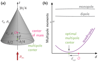
Figure 1: Sketch of the considered problem. (a) A cone of height $h$ under insonification of an acoustic plane wave propagating along the $z$-axis. The center of the multipole expansion (green point) is offset from the center of mass (pink point $O$, $z=0$) by a distance $d$. (b) First three multipole moments of the cone vs. $d$ at a fixed frequency. The quadrupole moment exhibits a minimum, whereas the sum of the monopole and dipole moments has a maximum, manifesting the optimal multipole center’s position $z=d_{\rm opt}$.

Our study addresses this challenge in acoustics by seeking to minimize the number of multipoles retained in the expansion when describing the acoustic scattering response from either scatterers or finite arrays thereof. Through both analytical and numerical approaches, we examine the scattering of acoustic pressure waves by subwavelength scatterers to determine the location of the optimal multipole center (OMC). We demonstrate that selecting this optimal center minimizes the quadrupole contribution, creating ideal conditions for applying the monopole-dipole approximation (MDA) in acoustics widely used in the literature. Silva (2014); Toftul et al. (2019); Wei and Rodríguez-Fortuño (2020); Long et al. (2020); Smagin et al. (2024) This approach can be applied to both isolated scatterers and compact arrays where simple multipole sources interact at short distances.

We begin with a mathematical formulation of our problem. The scattered pressure $p_{\rm sca}(k;\mathbf{r})$ of an acoustical scatterer can be expanded into a truncated series of scalar spherical waves (multipoles) weighted with multipole moments Blackstock (2000)

$$p_{\rm sca}(k;\mathbf{r})=\sum_{\ell=0}^{\ell_{\rm max}}\sum_{m=-\ell}^{\ell}p_{\ell,m}(k;\mathbf{d})\psi^{(3)}_{\ell,m}(k;\mathbf{r}-\mathbf{d})\,.$$ (1)

$\ell$ and $m$ is the order and degree of the singular multipole $\psi^{(3)}_{\ell,m}(k;\mathbf{r}-\mathbf{d})$ [see Sec. S1A in Supplementary material (SM) for its definition]. $\mathbf{r}\neq\mathbf{d}$, and $k=\omega/c_{0}$ is the wavenumber in the surrounding medium. $\mathbf{d}$ is an offset of the multipole center relative to the scatterer’s center of mass defined as $\mathbf{r}_{\rm CM}=\bm{0}$ [point $O$ in Fig. 1(a)]. We always want to choose the optimal $\mathbf{d}_{\rm opt}$ that simultaneously provides the best precision for calculating the physical quantities and the lowest maximal multipole order $\ell_{\rm max}$ in the expansion. In this work, we assume that the offset $\mathbf{d}$ is subwavelength, that is, $\mathbf{kd}\ll 1$.

To determine $\mathbf{d}_{\rm opt}$, we need to know the dependence of the multipole moments on $\mathbf{d}$. Using the translation coefficients of spherical waves $\alpha^{(1)}_{\ell m\ell^{\prime}m^{\prime}}(k;\mathbf{d})$ [Sec. S1C in SM], Martin (2006) we link the multipole moments obtained for an expansion center shifted to $\mathbf{d}$ to the multipole moments obtained at the center of mass, i.e., at $\mathbf{d}=\bm{0}$ [see Sec. S1D in SM]

$$p_{\ell,m}(k;\mathbf{d})=\sum_{\ell^{\prime}=0}^{\ell_{\rm max}}\sum_{m^{\prime}=-\ell^{\prime}}^{\ell^{\prime}}\alpha^{(1)}_{\ell m\ell^{\prime}m^{\prime}}(k;\mathbf{d})p_{\ell^{\prime},m^{\prime}}(k;\bm{0})\,.$$ (2)

$p_{\ell^{\prime},m^{\prime}}(k;\bm{0})$ can be computed using, e.g., the acoustic T-matrix of the scatterer Waterman (1969, 2009) or upon post-processing simulations from a full-wave solver [see, e.g., Appendix B in Ref. Tsimokha et al., 2022]. Equation (2) is of significant practical importance – it shows that to obtain the entire dependence of the multipole moments on $\mathbf{d}$, we can calculate the multipole moments only once, if the chosen $\ell_{\rm max}$ is sufficient.

Further, we verify our semi-analytical approach in two examples. As a first example, we find the OMC for a cone-shaped scatterer with cylindrical symmetry along the $z$-axis [see Fig. 1(a)]. The symmetry is conserved for a plane wave excitation along the $z$-axis, and only the zonal multipoles (with $m=0$) are excited. Moreover, the offset along the $z$-axis $\mathbf{d}=d\hat{\mathbf{z}}$ affects only the zonal multipole content of the scatterer because the shifted system remains axisymmetric. Furthermore, we consider a spectral range where the first three multipoles sufficiently approximate the scattering for all $d$ we examine, i.e., $\ell_{\rm max}=2$ can be held. In this case, the scattering cross-section of the cone is $\sigma_{\rm tot}(k)=k^{-2}\sum_{\ell=0}^{\ell_{\rm max}}|p_{\ell,0}(k;\mathbf{d})|^{2}$. Here, we consider the offsets $d$ that are sufficiently small to make $\sigma_{\rm tot}(k)$ almost independent on $\mathbf{d}$, while its MDA $\sigma_{\rm md}(k;\mathbf{d})=k^{-2}\sum_{\ell=0}^{1}|p_{\ell,0}(k;\mathbf{d})|^{2}$ still depends on $\mathbf{d}$. Therefore, we define $\mathbf{d}_{\rm opt}$ as $\min_{\mathbf{d}}|p_{2,0}(k;\mathbf{d})|^{2}$ for a given $k$ to reduce error $|\sigma_{\rm md}(k;\mathbf{d})-\sigma_{\rm tot}(k)|$. We then compute $\mathbf{d}_{\rm opt}$ from equation $\bm{\nabla}_{\mathbf{d}}|p_{2,0}(k;\mathbf{d})|^{2}=0$.

Although standard numerical methods Chong and Żak (2013) can be used to find $\mathbf{d}_{\rm opt}$, we solve this problem analytically. We start by adapting (2) to the considered case and write the off-origin quadrupole moment as a function of a normalized offset $d_{k}=kd$. For all zonal multipole coefficients, we use substitutions $p_{2}(d_{k})\equiv p_{2,0}(k;d\hat{\mathbf{z}})$, and $p_{\ell}\equiv p_{\ell,0}(k;\bm{0})$ for brevity, and then arrive at the following compact equation

$$\begin{aligned} p_{2}(d_{k})=p_{2}+\mathbf{A}_{2}(d_{k})\cdot\mathbf{p}\,,\end{aligned}$$ (3)

with $\mathbf{p}=\begin{bmatrix}p_{0},p_{1},p_{2}\end{bmatrix}^{\rm T}$, $\mathbf{A}_{2}(d_{k})=\begin{bmatrix}\alpha_{0}(d_{k}),\alpha_{1}(d_{k}),\alpha_{2}(d_{k})\end{bmatrix}^{\rm T}$, and $\alpha_{\ell^{\prime}}(d_{k})\equiv\alpha^{(1)}_{20\ell^{\prime}0}(k;d\hat{\mathbf{z}})-\delta_{2,\ell^{\prime}}$. The long-wavelength approximation (LWA) $kd\ll 1$ of the spherical Bessel functions [see Sec. S1B in SM] gives an approximate separation vector $\widetilde{\mathbf{A}}_{2}(d_{k})=\begin{bmatrix}\widetilde{\alpha}_{0}(d_{k}),\widetilde{\alpha}_{1}(d_{k}),\widetilde{\alpha}_{2}(d_{k})\end{bmatrix}^{\rm T}$

$$\begin{aligned} \widetilde{\mathbf{A}}_{2}(d_{k})=\begin{bmatrix}\frac{1}{3\sqrt{5}}d_{k}^{2},-\frac{2}{\sqrt{15}}d_{k},-\frac{11}{42}d_{k}^{2}\end{bmatrix}^{\rm T}\,,\end{aligned}$$ (4)

where the tilde is used to distinguish the accurate values of translation coefficients $\alpha_{\ell^{\prime}}$ from their LWA $\widetilde{\alpha}_{\ell^{\prime}}$. After substituting (4) into (3), we arrive at a quadratic approximation of $|p_{2}(d_{k})|^{2}$

$$|\tilde{p}_{2}(d_{k})|^{2}=f_{0,k}+f_{1,k}d_{k}+f_{2,k}d_{k}^{2}+\mathcal{O}(d_{k}^{3})\,,$$ (5)

where $f_{0,k}=|p_{2}|^{2}$, $f_{1,k}=-\frac{4}{\sqrt{15}}\Re\left[p_{1}^{*}p_{2}\right]$, and $f_{2,k}=\frac{4}{15}|p_{1}|^{2}-\frac{11}{21}|p_{2}|^{2}+\frac{2}{3\sqrt{5}}\Re\left[p_{0}^{*}p_{2}\right]$ with a real $k$ [for a complex $k$, we refer to Sec. S2C in SM] and $p_{\ell}=p_{\ell}(k)$, calculated for $d=0$. The accuracy of Eqs. (3) and (5) in the considered spectral range is confirmed in Sec. S2A in SM. Similar interpolations can be derived for the coefficients $p_{0}(d_{k})$ and $p_{1}(d_{k})$ [see Sec. S2B in SM] as well as for high-order terms. The main outcome of (5) is an analytical formula for the optimal offset being a solution to the equation $\partial_{d_{k}}|\tilde{p}_{2}(d_{k})|^{2}=0$ ($k$ is fixed) that provides $d_{\rm opt}=-f_{1,k}/\left(2kf_{2,k}\right)$, or

$$d_{\rm opt}=\frac{\sqrt{3}}{k}\frac{\Re\left[p_{1}^{*}p_{2}\right]}{\frac{2}{\sqrt{5}}|p_{1}|^{2}-\frac{11\sqrt{5}}{14}|p_{2}|^{2}+\Re\left[p_{0}^{*}p_{2}\right]}\,,$$ (6)

where the sign of the second derivative $f_{2,k}>0$ and $k\neq 0$ have been implied. Thus, once the multipole moments at $d=0$ are known, the OMC’s position is directly given by (6). Moreover,  (6) can be used even if the initial multipole center is at an arbitrary point $d=d_{0}$. Then, a translation $\left(d_{\rm opt}+d_{0}\right)$ gives the OMC.

To increase the accuracy, one can extend expansion (5) up to the next even power of $kd$

$$|\breve{p}_{2}(d_{k})|^{2}=\sum_{n=0}^{4}f_{n,k}(d_{k})^{n}+\mathcal{O}(d_{k}^{5}),$$ (7)

where $f_{3,k}$ and $f_{4,k}$ are given in Sec. S2C in SM. In this case, an optimal offset is calculated as a pure real solution to the cubic equation $\partial_{d_{k}}|\breve{p}_{2}(d_{k})|^{2}=0$

$$f_{1,k}+2f_{2,k}d_{k}+3f_{3,k}d_{k}^{2}+4f_{4,k}d_{k}^{3}=0.$$ (8)

To validate the analytical results, we perform a numerical simulation of the scattering of a plane wave by a cone of height $h=1$ cm and a radius of $h/2$. The cone is made of a material with the speed of sound $c_{1}$ and mass density $\rho_{1}$. It is placed in a medium with $c_{0}/c_{1}=\sqrt{21}$ and $\rho_{0}/\rho_{1}=1/7$ [see Fig. 1(a)]. We use our in-house T-matrix-based code acoustotreams, aco which is an adaptation of the electromagnetic scattering code treams for acoustic scattering. Beutel, Fernandez-Corbaton, and Rockstuhl (2024) The acoustic T-matrix of the cone was calculated for $d=0$ in a spectral range between 5-25.5 kHz with a step of 0.1 kHz using the finite-element method (Pressure Acoustics interface in COMSOL Multiphysics, v. 6.2). com The acoustic T-matrix was then exported to acoustotreams to calculate the offset multipole moments (2) with $\ell_{\rm max}=7$ (full-wave model).

Figure 2 presents the results of the full-wave numerical simulations, which are the cone scattering efficiency in (a), the normalized quadrupole moment map in (b) with numerical values of $d_{\rm opt}$ shown by green markers, and the relative error for the MDA of the scattering cross-section in (c) calculated for the multipole center placed at the center of mass and OMC (numerical values). Figure 2(b) also compares the numerical values of $d_{\rm opt}$ to the analytical values in the quadratic (6) and quartic (8) approximations, respectively. Multiple observations can be made.

First, the OMC converges to $d_{\rm opt}=-0.075$ cm in a subwavelength regime $\omega h/c_{0}\lesssim 1$ [see Fig. 2(b)]. Thus, the OMC is located below the center of mass, similar to the magnetic multipole center of electromagnetic scatterers. Kildishev, Achouri, and Smirnova (2024) The OMCs predicted by all three models coincide for $\omega h/c_{0}<2.75$ except at the monopole resonance $\omega_{\rm I}h/c_{0}=1.7$. For optical scatterers, we have already demonstrated that the optimal multipole center differs from the scatterer’s center of mass and is, in fact, dispersive Kildishev, Achouri, and Smirnova (2024). In contrast, at dipole resonance $\omega_{\rm II}h/c_{0}=2.4$, all models predict the same OMC with a significant suppression of the error [see the inset in Fig. 2(c)]. In Fig. 2(b), we also see that the negative OMC turns into a large positive OMC around $\omega_{\rm III}h/c_{0}\simeq 2.75$ (the gray region in Fig. 2), and the second derivatives of (5) and (7) become negative [see Sec. S3 in SM]. In this case, the monopole contribution to the scattering is suppressed, while the quadrupole becomes substantial. Figure 2(c) also confirms that neglecting the quadrupole around $\omega\simeq\omega_{\rm III}$ leads to an error larger than $40$%. Hence, the OMC should be redefined as a minimum of a higher-order multipole moment. Surprisingly, at the quadrupole resonance $\omega_{\rm IV}h/c_{0}=3.24$, the quadrupole moment can still be neglected with an error of $10$% since the monopole also exhibits a resonant-like response. Thus, a center for the multipole expansion of the fields placed at the optimal point provides the best conditions for MDA. The error in the scattering cross-section is consistently smaller when the OMC is chosen for the expansion compared to when the center of mass is chosen [see Fig. 2(c)]. At the same time, one can use Eq. (6) to predict the positions of the OMC for $\omega h/c_{0}\leq 2.75$ when $f_{2,k}>0$. For higher frequencies, Eq. (8) should be employed [see Fig. 2(b)].

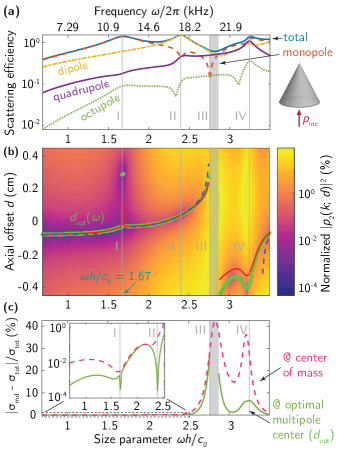
Figure 2: (a) Scattering efficiency $\sigma_{\rm tot}(k)/(0.25\pi h^{2})$ of the cone, shown in the inset, with its multipole decomposition for the multipole center at $d=0$. (b) Normalized zonal quadrupole moment of the cone $|p_{2}(k;d)|^{2}/\sum_{\ell\neq 2}|p_{\ell}(k;d)|^{2}$ for $\ell_{\rm max}=7$. The green dots show the values of $d_{\rm opt}=\min_{d}|p_{2}(k;d)|^{2}$, obtained directly from the full-wave numerical simulations. The dashed cyan and solid red lines show $d_{\rm opt}$ calculated with the quadratic [Eq. (6)] and quartic [Eq.  (8)] approximations of $|p_{2}(k;d)|^{2}$, respectively. (c) Error of the scattering cross-section for $\ell_{\rm max}=1$ relative to that for $\ell_{\rm max}=7$ at $d=0$ (pink dashed) and $d=d_{\rm opt}$, calculated in the full-wave model (green solid). Inset: the same but on a logarithmic scale for $\omega h/c_{0}\leq 2.5$.

In a further analysis, we demonstrate that the OMC can be found not only for individual scatterers but also for finite arrangements thereof. The framework of the T-matrix method can be efficiently applied to acoustic multi-scattering problems Peterson and Ström (1975); Kafesaki and Economou (1999); Psarobas, Stefanou, and Modinos (2000), where one needs to distinguish a formulation in a local and global description of the scattered fields of the arrangements Suryadharma et al. (2017). In the local description (LD), the fields are expanded at the $N$ local positions of all $N$ scatterers, $\mathbf{r}_{i}$ with $i=1..N$. The multiple scattering equation is solved to obtain the self-consistent multipole moments that account for the interactions of the scatterers with the incident field and with each other [see, e.g., (17) in Ref. Beutel, Fernandez-Corbaton, and Rockstuhl, 2024]. In the global description (GD), the fields are expanded from all particles using a global expansion center at a single point $\mathbf{d}$

$$p^{\rm(global)}_{\ell,m}(k;\mathbf{d})=\sum_{\ell^{\prime}=0}^{\ell_{\rm max}}\sum_{m^{\prime}=-\ell^{\prime}}^{\ell^{\prime}}\sum_{i=1}^{N}\alpha^{(1)}_{\ell m\ell^{\prime}m^{\prime}}(k;\mathbf{d}-\mathbf{r}_{i})p_{\ell^{\prime},m^{\prime}}^{\rm(local)}(k;\mathbf{r}_{i})\,.$$ (9)

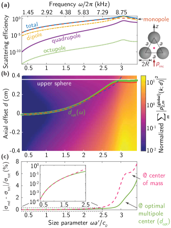
Figure 3: The same as in Fig. 2 but for a trimer of spherical scatterers [see the inset of panel (a)] using the global description (9) of the trimer acoustic response. (a) The scattering efficiency is $\sigma_{\rm tot}(k)/(0.25\pi[a^{\prime}]^{2})$ where $a^{\prime}=a+2R$. The pink dot indicates the center of mass. (b) Normalized global quadrupole moment of the trimer $\sum_{m}|p^{\rm(global)}_{2,m}(k;d)|^{2}/\sum_{\ell\neq 2,m}|p^{\rm(global)}_{\ell,m}(k;d)|^{2}$ for $\ell_{\rm max}=2$ and $L_{\rm max}=4$. The green dots show the values of $d_{\rm opt}=\min_{d}\sum_{m}|p^{\rm(global)}_{2,m}(k;d)|^{2}$, obtained directly from the full-wave numerical simulations. The dashed cyan and solid red lines show $d_{\rm opt}$ calculated with the quadratic [Eq. (6)] and quartic [Eq. (8)] approximations of the zonal term $|p^{\rm(global)}_{2,0}(k;d)|^{2}$, respectively. (c) Error of the scattering cross-section for $L_{\rm max}=1$ relative to that for $L_{\rm max}=4$ at $d=0$ (pink dashed) and $d=d_{\rm opt}$, calculated in the full-wave model (green solid). Inset: the same but on a logarithmic scale for $\omega a^{\prime}/c_{0}\leq 2.5$.

Equation (9) is similar to (2) for a single-particle case but with the sum over different particles. The other feature is more inconspicuous. The maximal multipole order in the GD $L_{\rm max}$ can be larger than in the LD $\ell_{\rm max}$. Thus, the transition from the LD to the GD is reasonable when the size of an arrangement T-matrix in the GD, $(L_{\rm max}+1)^{2}$, is smaller than the size of an arrangement T-matrix in the LD, $N(\ell_{\rm max}+1)^{2}$.

As an example, we consider a trimer of spherical particles shown in Fig. 3(a). The spheres of radius $R=0.5$ cm are placed at the nodes of an equilateral triangle of side $a=3R$. The material parameters (mass density and speed of sound) of the scatterer material and background are the same as before. Hereafter, we can use the same formalism as before but in a multi-scattering scenario to find the minima of the quadrupole moment in the GD $\sum_{m=-2}^{2}|p^{\rm(global)}_{2,m}(k;\mathbf{d})|^{2}$. An interaction between the spheres can induce the multipoles with $m\neq 0$. However, their contribution is smaller than that of zonal multipoles. Therefore, we can apply Eqs. (6) and (8) to predict $d_{\rm opt}$. We assume the range of frequencies 1–11 kHz where $\ell_{\rm max}=1$ and $L_{\rm max}=2$ are sufficient. If we manage to find the OMC where even $L_{\rm max}=1$ provides good accuracy, then we will decrease the size of the trimer T-matrix from 12 to 4, although one has to track $d_{\rm opt}(\omega)$.

Figure 3 presents the same content as Fig. 2 but for the trimer. The main difference lies in the behavior of $d_{\rm opt}$. In the static case, the system is symmetric concerning the rotations by $\pi/3$ and $2\pi/3$ in the $xz$ plane; hence $d_{\rm opt}\to 0$ when $\omega a^{\prime}/c_{0}\to 0$, i.e., the OMC coincides with the center of mass [see Fig. 3(b)]. Here, $\omega a^{\prime}/c_{0}$ is an effective trimer size parameter with $a^{\prime}=a+2R$. As $\omega a^{\prime}/c_{0}$ increases, $d_{\rm opt}$ also increases. From $\omega a^{\prime}/c_{0}=2.6$, the OMC remains at the same point $d_{\rm opt}\approx 0.35$ cm close to the center of the upper sphere and provides a better accuracy of the MDA [see Fig. 3(c)]. Both quadratic and quartic models predict $d_{\rm opt}$ for $\omega a^{\prime}/c_{0}\leq 2.6$ very well, although the quadratic model fails for $\omega a^{\prime}/c_{0}>2.6$ due to the resonant response of the trimer [see Fig. 3(a)]. In Sec. S4 in SM, we also consider this trimer rotated by $\pi/2$ in the $xz$ plane, for which $\mathbf{d}_{\rm opt}$ is traced as a trajectory, with the initial point at $\mathbf{d}_{\rm opt}=\bm{0}$, as the frequency increases.

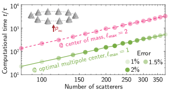
Figure 4: Normalized computational time versus the number of cone-shaped scatterers arranged in a ring depicted in the inset. The expansion center for the single cone is placed at either its center of mass with $\ell_{\rm max}=2$ (pink dashed) or the OMC with $\ell_{\rm max}=1$ (green solid). The transparency of the markers indicates the corresponding error of the scattering cross-section.

In the end, we demonstrate that the OMC can improve the computational efficiency of the acoustic T-matrix method in multiple scattering problems. For that purpose, we consider a ring of the $N$ identical cones (the same as those previously considered) placed at a distance $D=2.6$ cm between the nearest neighbors. The acoustic T-matrix of the individual cone is calculated at frequency $\omega h/c_{0}=2.5$ for the multipole expansion center placed at $d=0$ with $\ell_{\rm max}=2$, and at the OMC with $\ell_{\rm max}=1$ [see Fig. 2(b)]. An additional modification of the OMCs due to the interaction between scatterers is neglected. Then, we vary $N$ from 80 to 380, estimate the time we need to solve the multiple scattering problem, compute the ring scattering cross section for each $N$, average this time after 10 iterations, and normalize it by $\tau$. Here, $\tau$ is the average time to solve a linear system with a $1000\times 1000$ matrix and $1000\times 1$ right-hand side using the numpy.linalg.solve function in Python 3.11.

Figure 4 illustrates the results, demonstrating that the OMC reduces computational time by six since we manage to reduce the size of the isolated-cone T matrix from 9 for $\ell_{\rm max}=2$ to 4 for $\ell_{\rm max}=1$, while the error in the calculation of the ring scattering cross-section remains comparable. Moreover, using the MDA but placing the multipole center at the center of mass increases the average error from 1.42% to 4%. Thus, the OMC remarkably reduces the computational time within the T-matrix and multipole methods for simulating the acoustic response of discrete scatterers while maintaining a reasonable error.

As drawbacks of the OMC approach, we have to mention first that an offset $d$ of the multipole expansion center effectively increases the radius of a sphere circumscribing the scatterer from $R_{\mathrm{c}}$ to $(R_{\mathrm{c}}+d)$. Expansion (1) becomes then valid outside a larger circumscribing sphere, Auguié et al. (2016) which may lead to larger minimal spacings between the scatterers in their arrangements. Moreover, the OMC, as discussed here, has been found for a particular incidence of the external wave along the $z$-axis. As discussed in Ref. Kildishev, Achouri, and Smirnova, 2024, a different illumination direction leads to different OMCs, making the OMC both frequency- and angular-dispersive [see Sec. S5 in SM].

In conclusion, we address the problem of determining the optimal point to place the center of the multipole expansion in acoustic scattering. We consider individual scatterers and multiple-particle structures without reflection symmetry along the $z$-axis and trace the OMC position along the axis upon insonification of the scatterers with a plane wave. Our comprehensive acoustic scattering model reveals that similar to electromagnetic scattering, Kildishev, Achouri, and Smirnova (2024) an optimal solution that minimizes the multipole content to produce the most efficient descriptor while retaining only a few terms of the lowest degree. We showcase the advantages of using low-degree multipoles (monopole and dipole) at this OMC, demonstrating substantial computational efficiency gains achieved in T-matrix calculations. Our approach can be extended beyond the systems described with the monopole-dipole-quadrupole approximation to systems that require optimizing their multipole descriptions up to arbitrary degrees and orders.

See the Supplementary material for the definition of scalar spherical waves (multipoles), the addition theorem and translation coefficients, the derivation of Eqs. (3)-(8), the analysis of the error of the approximations (3),  (4), and (7), calculation of an optimal multipole center trajectory for the rotated trimer, and the calculation of an optimal multipole center for the isolated cone as a function of the angle of incidence.

Data Availability Statement

The data that support the findings of this study are openly available on GitHub at https://github.com/NikUstimenko/acoustotreams.git, Ref. aco, .

References

- Kinsler et al. (1999) L. E. Kinsler, A. R. Frey, A. B. Coppens, and J. V. Sanders, Fundamentals of Acoustics (4th Edition) (John Wiley & Sons Inc, Hoboken, NJ, USA, 1999).
- Sainidou et al. (2005) R. Sainidou, N. Stefanou, I. E. Psarobas, and A. Modinos, Comput. Phys. Commun. 166, 197 (2005).
- Gong et al. (2017) Z. Gong, W. Li, Y. Chai, Y. Zhao, and F. G. Mitri, Ocean Eng. 129, 507 (2017).
- Gong, Marston, and Li (2019) Z. Gong, P. L. Marston, and W. Li, Phys. Rev. E 99, 063004 (2019).
- Ganesh and Hawkins (2022) M. Ganesh and S. C. Hawkins, J. Acoust. Soc. Am. 151, 1978 (2022).
- Yang et al. (2023) Y. Yang, Q. Gui, Y. Zhang, Y. Chai, and W. Li, Front. Phys. 11, 1170811 (2023).
- Li, Han, and Hu (2024) Z. Li, P. Han, and G. Hu, J. Mech. Phys. Solids 189, 105692 (2024).
- Haberman and Guild (2016) M. R. Haberman and M. D. Guild, Phys. Today 69, 42 (2016).
- Wang et al. (2016) Z. Wang, Q. Zhang, K. Zhang, and G. Hu, Adv. Mater. 28, 9857 (2016).
- Bertoldi et al. (2017) K. Bertoldi, V. Vitelli, J. Christensen, and M. van Hecke, Nat. Rev. Mater. 2, 1 (2017).
- Sieck, Alù, and Haberman (2017) C. F. Sieck, A. Alù, and M. R. Haberman, Phys. Rev. B 96, 104303 (2017).
- Colton and Kress (2019) D. Colton and R. Kress, Inverse Acoustic and Electromagnetic Scattering Theory (Springer International Publishing, Cham, Switzerland, 2019).
- Ronellenfitsch et al. (2019) H. Ronellenfitsch, N. Stoop, J. Yu, A. Forrow, and J. Dunkel, Phys. Rev. Mater. 3, 095201 (2019).
- Krishna et al. (2022) A. Krishna, S. R. Craig, C. Shi, and V. R. Joseph, Appl. Phys. Lett. 121 (2022), 10.1063/5.0096869.
- Long et al. (2022) H. Long, Y. Zhu, Y. Gu, Y. Cheng, and X. Liu, Phys. Rev. Appl. 18, 044032 (2022).
- Li et al. (2023) Z. Li, Y. Sun, G. Wu, and M. Tao, Appl. Acoust. 204, 109247 (2023).
- Fang et al. (2024) B. Fang, R. Zhang, T. Chen, W. Wang, J. Zhu, and W. Cheng, Journal of Building Engineering 86, 108898 (2024).
- Zhan et al. (2018) A. Zhan, T. K. Fryett, S. Colburn, and A. Majumdar, Appl. Opt. 57, 1437 (2018).
- Zhelyeznyakov, Zhan, and Majumdar (2020) M. V. Zhelyeznyakov, A. Zhan, and A. Majumdar, OSA Continuum 3, 89 (2020).
- Ustimenko et al. (2021) N. Ustimenko, K. V. Baryshnikova, R. Melnikov, D. Kornovan, V. Ulyantsev, B. N. Chichkov, and A. B. Evlyukhin, J. Opt. Soc. Am. B 38, 3009 (2021).
- Gladyshev et al. (2023) S. Gladyshev, T. D. Karamanos, L. Kuhn, D. Beutel, T. Weiss, C. Rockstuhl, and A. Bogdanov, Nanophotonics 12, 3767 (2023).
- Garg et al. (2024) P. Garg, J. D. Fischbach, A. G. Lamprianidis, X. Wang, M. S. Mirmoosa, V. S. Asadchy, C. Rockstuhl, and T. J. Sturges, arXiv (2024), 10.48550/arXiv.2409.04551.
- Clebsch (1863) A. Clebsch, De Gruyter 1863, 195 (1863).
- Lorenz (2019) L. Lorenz, Eur. Phys. J. H 44, 77 (2019).
- Mie (1908) G. Mie, Ann. Phys. 330, 377 (1908).
- Mühlig et al. (2011) S. Mühlig, C. Menzel, C. Rockstuhl, and F. Lederer, Metamaterials 5, 64 (2011).
- Fernandez-Corbaton et al. (2015) I. Fernandez-Corbaton, S. Nanz, R. Alaee, and C. Rockstuhl, Opt. Express 23, 33044 (2015).
- Evlyukhin et al. (2016) A. B. Evlyukhin, T. Fischer, C. Reinhardt, and B. N. Chichkov, Phys. Rev. B 94, 205434 (2016).
- Smirnova and Kivshar (2016) D. Smirnova and Y. S. Kivshar, Optica 3, 1241 (2016).
- Zhu et al. (2016) X. Zhu, B. Liang, W. Kan, Y. Peng, and J. Cheng, Phys. Rev. Appl. 5, 054015 (2016).
- Alaee, Rockstuhl, and Fernandez-Corbaton (2018) R. Alaee, C. Rockstuhl, and I. Fernandez-Corbaton, Opt. Commun. 407, 17 (2018).
- Alaee, Rockstuhl, and Fernandez-Corbaton (2019) R. Alaee, C. Rockstuhl, and I. Fernandez-Corbaton, Adv. Opt. Mater. 7, 1800783 (2019).
- Kovacevich and Popa (2021) D. A. Kovacevich and B.-I. Popa, Phys. Rev. B 104, 134304 (2021).
- Riccardi et al. (2022) M. Riccardi, A. Kiselev, K. Achouri, and O. J. F. Martin, Phys. Rev. B 106, 115428 (2022).
- Auguié et al. (2016) B. Auguié, W. R. C. Somerville, S. Roache, and E. C. Le Ru, J. Opt. 18, 075007 (2016).
- Evlyukhin, Reinhardt, and Chichkov (2011) A. B. Evlyukhin, C. Reinhardt, and B. N. Chichkov, Phys. Rev. B 84, 235429 (2011).
- Evlyukhin et al. (2013) A. B. Evlyukhin, C. Reinhardt, E. Evlyukhin, and B. N. Chichkov, J. Opt. Soc. Am. B 30, 2589 (2013).
- Silva (2014) G. T. Silva, J. Acoust. Soc. Am. 136, 2405 (2014).
- Toftul et al. (2019) I. D. Toftul, K. Y. Bliokh, M. I. Petrov, and F. Nori, Phys. Rev. Lett. 123, 183901 (2019).
- Wei and Rodríguez-Fortuño (2020) L. Wei and F. J. Rodríguez-Fortuño, New J. Phys. 22, 083016 (2020).
- Long et al. (2020) Y. Long, H. Ge, D. Zhang, X. Xu, J. Ren, M.-H. Lu, M. Bao, H. Chen, and Y.-F. Chen, Natl. Sci. Rev. 7, 1024 (2020).
- Smagin et al. (2024) M. Smagin, I. Toftul, K. Y. Bliokh, and M. Petrov, Phys. Rev. Appl. 22, 064041 (2024).
- Blackstock (2000) D. T. Blackstock, Fundamentals of Physical Acoustics (Wiley, Hoboken, NJ, USA, 2000).
- Martin (2006) P. A. Martin, Multiple Scattering: Interaction of Time-Harmonic Waves with Obstacles (Cambridge University Press, Cambridge, England, UK, 2006).
- Waterman (1969) P. C. Waterman, J. Acoust. Soc. Am. 45, 1417 (1969).
- Waterman (2009) P. C. Waterman, J. Acoust. Soc. Am. 125, 42 (2009).
- Tsimokha et al. (2022) M. Tsimokha, V. Igoshin, A. Nikitina, I. Toftul, K. Frizyuk, and M. Petrov, Phys. Rev. B 105, 165311 (2022).
- Chong and Żak (2013) E. K. P. Chong and S. H. Żak, An Introduction to Optimization (Wiley, Chichester, England, UK, 2013).
- (49) https://github.com/NikUstimenko/acoustotreams.git.
- Beutel, Fernandez-Corbaton, and Rockstuhl (2024) D. Beutel, I. Fernandez-Corbaton, and C. Rockstuhl, Comput. Phys. Commun. 297, 109076 (2024).
- (51) https://www.comsol.com/acoustics-module.
- Kildishev, Achouri, and Smirnova (2024) A. V. Kildishev, K. Achouri, and D. Smirnova, Adv. Opt. Mater. n/a, 2402787 (2024).
- Peterson and Ström (1975) B. Peterson and S. Ström, J. Acoust. Soc. Am. 57, 2 (1975).
- Kafesaki and Economou (1999) M. Kafesaki and E. N. Economou, Phys. Rev. B 60, 11993 (1999).
- Psarobas, Stefanou, and Modinos (2000) I. E. Psarobas, N. Stefanou, and A. Modinos, Phys. Rev. B 62, 278 (2000).
- Suryadharma et al. (2017) R. N. S. Suryadharma, M. Fruhnert, I. Fernandez-Corbaton, and C. Rockstuhl, Phys. Rev. B 96, 045406 (2017).