The ultraviolet luminosity function of star-forming galaxies between redshifts of 0.4 and 0.6

Abstract

We combine ultraviolet imaging of the $13^{H}$ survey field, taken with the XMM-Newton Optical Monitor telescope (XMM-OM) and the Neil Gehrels Swift Observatory Ultraviolet and Optical Telescope (UVOT) in the UVM2 band, to measure rest-frame ultraviolet 1,500 Å luminosity functions of star-forming galaxies with redshifts $z$ between 0.4 and 0.6. In total the UVM2 imaging covers a sky area of 641 arcmin², and we detect 273 galaxies in the UVM2 image with $0.4<z<0.6$. The luminosity function is fit by a Schechter function with best-fit values for the faint end slope $\alpha=-1.8^{+0.4}_{-0.3}$ and characteristic absolute magnitude $M^{*}=-19.1^{+0.3}_{-0.4}$. In common with XMM-OM based studies at higher redshifts, our best-fitting value for $M^{*}$ is fainter than previous measurements. We argue that the purging of active galactic nuclei from the sample, facilitated by the co-spatial X-ray survey carried out with XMM-Newton is important for the determination of $M^{*}$. At the brightest absolute magnitudes ($M_{1500}<-18.5$) the average UV colour of our galaxies is consistent with that of minimal-extinction local analogues, but the average UV colour is redder for galaxies at fainter absolute magnitudes, suggesting that higher levels of dust attenuation enter the sample at absolute magnitudes somewhat fainter than $M^{*}$.

1 Introduction

Luminosity functions, the space density per unit luminosity interval as a function of luminosity, are one of the most fundamental characterisations of any astronomical population. Luminosity functions can be defined for luminosities measured at any rest-frame wavelength. At optical wavelengths, light from galaxies is contributed by stars of a variety of ages, and so the optical luminosity function of galaxies depends on the cumulative stellar processes in galaxies over large cosmic timescales. By contrast, at ultraviolet wavelengths the light from massive, young stars easily overwhelms the older stellar population, and so the luminosity is largely determined by recent ($\leq$100 Myr) star-formation activity (Kennicutt & Evans, 2012), hence the ultraviolet luminosity function of galaxies reflects the distribution of instantaneous star formation rates.

For luminosity functions at ultraviolet wavelengths, luminosity is usually described by absolute magnitude, and so the ultraviolet luminosity function is usually defined as

$$\phi=\frac{d^{2}N}{dVdM}$$ (1)

where $N$ is the number of galaxies, $V$ is volume of space and $M$ is absolute magnitude.

UV measurements have been a key means to identify and study the star-forming galaxy population, particularly at high redshift, since the Lyman-break technique was employed successfully in the 1990s (e.g. Steidel et al., 2006; Madau et al., 1996). Today, rest-frame UV selection remains key to the identification and population studies of the highest-redshift star-forming galaxies (e.g. Donnan et al., 2023; Pérez-González et al., 2023; Harikane et al., 2023), via infrared observations with the James Webb Space Telescope.

At low redshift, the use of ultraviolet observations to construct luminosity functions of galaxies was pioneered by Treyer et al. (1998) and Sullivan et al. (2000), utilising balloon-borne UV observations. They showed that the luminosity function is well represented by a Schechter function shape (Schechter, 1976). Major strides were made with the launch of GALEX (Martin et al., 2005), which facilitated the construction of UV luminosity functions all the way from $z=0$ to $z=1.2$ (Wyder et al., 2005; Arnouts et al., 2005), beyond which the rest-frame 1,500 Å ultraviolet region is sufficiently redshifted to be accessible with ground based observations. The utility of GALEX to detect faint galaxies at intermediate redshifts ($z>0.2$) is ultimately limited by its image resolution and the source confusion that becomes severe at the faintest magnitudes ($m_{NUV}>23.6$; Xu et al., 2005).

Both ESA’s XMM-Newton observatory, and NASA’s Neil Gehrels Swift Observatory (hereafter Swift) carry imaging UV telescopes with better image resolution than GALEX: the Optical Monitor (XMM-OM; Mason et al., 2001) and Ultraviolet and Optical Telescope (UVOT; Roming et al., 2005) respectively. Deep observations with the Swift UVOT have been used to construct UV luminosity functions between $z=0.2$ and $z=1.2$ (Hagen et al., 2015). Their luminosity functions were not limited by confusion, but colour-dependent selection effects result in faint absolute magnitude limits similar to those of Arnouts et al. (2005). More recently, Page et al. (2021), Sharma, Page & Breeveld (2022) and Sharma et al. (2024) have used XMM-OM observations taken with the UVW1 filter ($\lambda_{eff}=2910$ Å) to construct rest-frame 1,500 Å luminosity functions in the redshift range $0.6<z<1.2$, with Sharma, Page & Breeveld (2022) reaching significantly fainter absolute magnitudes than Arnouts et al. (2005) in this redshift range. These studies have highlighted the importance of excluding UV-bright active galactic nuclei (AGN) from the galaxy luminosity function to avoid contaminating the bright end.

Very recently, Bhattacharya, Saha & Mondal (2023) have used high-resolution images from the AstroSat Ultraviolet Imaging Telescope (UVIT; Tandon et al., 2017) and the Hubble Space Telescope (HST) to construct rest-frame 1,500 Å luminosity functions in the redshift range $0.4<z<0.8$, while Sun et al. (2023) used HST imaging to construct rest-frame 1,500 Å luminosity functions in the redshift range $0.6<z<1.0$. An earlier study by Oesch et. al. (2010) used HST data to construct a rest-frame 1,500 Å luminosity functions in the redshift range $0.5<z<1.0$. These HST and AstroSat studies reach fainter absolute magnitudes than the GALEX, XMM-OM or Swift UVOT studies.

This paper is based on a UV survey of galaxies in the 13^H Deep Field. The 13^H Deep Field is a patch of sky centred at 13^h 34^m 30^s $+37^{\circ}$ 53′ (J2000) with exceptionally low Galactic hydrogen column density, (${\rm N_{H}}\sim 7\times 10^{19}$ cm^-2; Branduardi-Raymont et al., 1994) and correspondingly low extinction (E(B-V)=0.005 mag; Schlafly & Finkbeiner, 2011). It is therefore very well suited for extragalactic surveys in the UV and soft X-ray. It was the location of the UK Rosat Deep Survey (McHardy et al., 1998) which was followed up with a long XMM-Newton exposure (Loaring et al., 2005) which includes UV observations with the XMM-OM (Page et al., 2021).

In this paper we build on the work of Page et al. (2021) by again constructing the UV galaxy luminosity function and examining the UV colours of galaxies, but this time in the more recent cosmic epoch corresponding to the redshift range $0.4<z<0.6$. UV luminosity functions have only been measured directly in this redshift range to date in three studies (Arnouts et al., 2005; Hagen et al., 2015; Bhattacharya, Saha & Mondal, 2023), of which two (Arnouts et al., 2005; Hagen et al., 2015) are likely affected by AGN contamination. Important questions include whether the UV luminosity function changes shape between cosmic noon and the present day, in the faint-end slope, or by diverging from the Schechter function shape at the luminous end, and the manner in which the UV luminosity function is shaped by extinction. At $z>2$ the colours of UV-selected galaxies become redder with luminosity (Bouwens et al., 2009), suggesting that extinction increases with UV luminosity, but this trend may not hold towards lower redshifts (Heinis et al., 2013) and there is some evidence for the opposite trend by $z=1$ (Sharma et al., 2024). Furthermore at $z>2$ the UV luminosity function exhibits a steepening of the faint-end slope with redshift (Reddy & Steidel, 2009; Bouwens et al., 2021), but at lower redshifts, after the peak in cosmic star formation, it is unclear if the shape is evolving.

For the redshift range $0.4<z<0.6$ we use images taken with the UVM2 filter of XMM-OM ($\lambda_{eff}=2310$ Å), which is better suited for the measurement of rest-frame 1,500 Å luminosity than the UVW1 filter. The 13^H Field has also been observed through the UVM2 filter of the Swift UVOT. The XMM-OM and UVOT have similar spatial resolution, employ similar photon-counting, microchannel-plate-intensified CCD detectors, and their UVM2 passband shapes are also similar (Fig. 1). Therefore, to expand the sky coverage and depth of the UVM2 imaging, we have combined the imaging from UVOT with that from XMM-OM.

Throughout this paper magnitudes are given in the AB system (Oke & Gunn, 1983), and we adopt Equation 1 as our definition for the luminosity function $\phi$. We have assumed cosmological parameters $H_{0}=70$ km s^-1 Mpc^-1, $\Omega_{\Lambda}=0.7$ and $\Omega_{\rm m}=0.3$. Unless stated otherwise, uncertainties are given at 1 $\sigma$.

2 Observations and data reduction

2.1 XMM-OM imaging

XMM-OM observed the 13^H field over three XMM-Newton orbits during June 2001. During these observations the XMM-OM took seven exposures through the UVM2 filter in Full-Frame Low-Resolution mode, each of 5000s duration. The observations are listed in Table 1. The XMM-OM images were initially processed with the XMM-Newton Science Analysis System (SAS) omichain to the stage of modulo-8 pattern noise correction. The images were then processed to remove the read-out streaks (Page et al., 2017) and an image of the UVM2 scattered-light background structure was subtracted from each exposure to flatten the background. The images were then distortion-corrected and re-projected in equatorial coordinates, and astrometrically matched to objects in the Sloan Digital Sky Survey Data Release 6 (Adelman-McCarthy et al., 2008) using the SAS task omatt. The images were then summed using the SAS task ommosaic.

Table 1: Observation log for UVM2 imaging. OBSID is the observation identification number. Exposure time gives the total UVM2 exposure for each OBSID, not corrected for dead-time.

OBSID	Date	Pointing Centre		Exposure
		RA (deg)	dec (deg)	(ks)
XMM-OM
0109660801	2001 Jun 12	203.665	37.913	20.00
0109660901	2001 Jun 22	203.665	37.913	5.00
0109661001	2001 Jun 24	203.665	37.913	10.00
Swift UVOT
00037657002	2008-08-12	203.631	37.787	10.17
00037657003	2008-08-13	203.668	37.773	8.32
00037658001	2011-02-17	203.690	37.750	1.74
00037658002	2011-11-04	203.672	37.782	0.49
00037658003	2011-11-09	203.640	37.796	0.19
00037658004	2011-11-13	203.628	37.795	0.85
00037658005	2011-12-07	203.656	37.773	3.57
00037658006	2012-09-03	203.664	37.809	1.69
00037658007	2012-10-17	203.625	37.804	0.66
00037658009	2013-05-18	203.624	37.713	0.22
00037658010	2013-09-03	203.657	37.780	0.21
00037658011	2013-10-17	203.619	37.796	2.89
00037658012	2013-10-19	203.648	37.793	0.38
00037658013	2013-11-01	203.644	37.795	0.81
00037658014	2013-12-07	203.643	37.782	1.51
00037658015	2013-12-12	203.654	37.776	0.49
00037658016	2013-12-20	203.666	37.773	0.87
00046361001	2014-10-18	203.673	38.043	0.71
00046361002	2019-09-06	203.615	38.035	0.11
00046361003	2019-10-25	203.667	38.050	0.51
00046361004	2019-11-02	203.691	38.056	0.42
00046361005	2019-11-03	203.657	38.035	0.72
00046361006	2021-10-17	203.658	38.068	0.07

2.2 Swift UVOT imaging

The 13^H field was observed with the Swift UVOT through the UVM2 filter over 23 observations between 2008 and 2021, for a total exposure of 37 ks. The pointing centres were spaced such that the UVOT observations cover a somewhat larger area than the XMM-OM observations. The observations are listed in Table 1. The UVOT images were processed with a combination of Swift ftools and bespoke tasks. Initially, the raw images from each observation were corrected for modulo-8 noise using the ftool uvotmodmap. Then the bad pixels at the corners and right-hand edge were masked, and the images were processed to remove the read-out streaks (Page et al., 2013). The images were then distortion-corrected and re-projected in equatorial coordinates using the ftool swiftxform. Exposure and large-scale sensitivity maps were created using the ftools uvotexpmap and uvotskylss. The images were then astrometrically matched to objects in the Sloan Digital Sky Survey Data Release 6, and the world coordinate systems in the exposure and large-scale sensitivity maps were updated accordingly.

2.3 Combining the XMM-OM and UVOT images

To combine the XMM-OM and UVOT images, various correction factors which would normally be accounted for during the source detection/photometry process were applied instead at the image stage. This methodology is incompatible with the corrections for coincidence-loss that are incorporated in the XMM-OM and UVOT photometry tasks. Coincidence-loss is the non-linearity that results from multiple incoming photons being indistinguishable from (and hence counted as) a single photon when they arrive in close proximity on the detector within a single image frame (Fordham, Moorhead & Galbraith, 2000). However, the galaxies that we are interested in are faint enough that coincidence-loss can be neglected.

First, the UVOT large-scale sensitivity correction was incorporated into the UVOT exposure maps by multiplying the exposure maps by the large scale sensitivity maps. Next the exposure maps for the XMM-OM and UVOT were divided by the appropriate time-dependent sensitivity correction factors. Next, the XMM-OM exposure map was divided by a factor of 2.826 to account for the difference in UVM2 zeropoints between XMM-OM and UVOT; see Appendix A for a full description of the origin of this factor. Then, the background count rates were measured in the XMM-OM and UVOT images. The background count rate was found to be higher in the XMM-OM image than in UVOT. UVM2 background in XMM-OM and UVOT is composed of dark current, zodiacal light and scattered light (Breeveld et al., 2010), and the enhanced background in XMM-OM is dominated by dark-current (Rosen et al., 2023). To equalise the XMM-OM and UVOT background count rates a constant was subtracted from the XMM-OM image. Changing the background in this way alters the noise properties of the image that would be inferred from the background counts, so the XMM-OM data were then down-weighted by dividing image and exposure by a constant factor to restore the original signal to noise properties for faint sources assuming Poisson statistics. The UVOT and XMM-OM images were then summed using the ftool uvotimsum. The exposure maps were combined in the same way. Finally, the images and exposure maps were converted to the format of a standard XMM-OM mosaic image. The combined UVM2 image is shown in Fig 2.

2.4 Source detection and characterisation

The combined XMM-OM and UVOT UVM2 image was searched for sources using the XMM-Newton SAS task omdetect. Photometry of sources which are consistent with the XMM-OM point-spread function is conducted using apertures of radius 2.8 to 5.6 arcseconds depending on brightness and the proximity of other sources. Photometry of extended sources is obtained from connected pixels which exceed a threshold above the background. For a more complete description of omdetect see Page et al. (2012). In practice, the majority of galaxies with $z>0.4$ are expected to appear point-like to XMM-OM and UVOT. A total of 1386 sources with a signal to noise ratio $\geq 4$ were detected in the UVM2 image.

Figure 1: Effective areas as a function of wavelength of the XMM-OM and Swift UVOT UVM2 passbands.

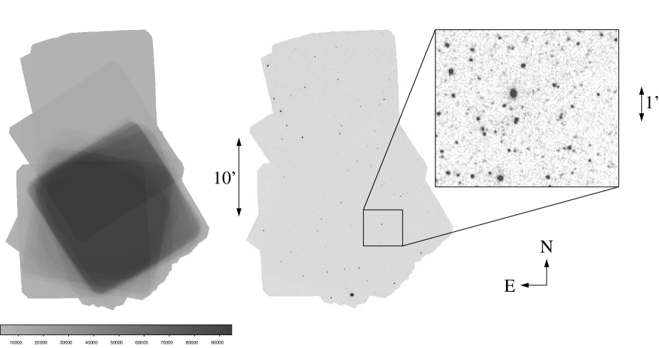
Figure 2: Combined XMM-OM and UVOT UVM2 exposure map and image of the 13^H field. The exposure map is shown on the left; the colour bar indicates the exposure time in seconds. The image is shown in centre. The highlighted region of the image is shown at larger scale on the right to demonstrate the quality of the image.

2.5 Completeness

In order to construct a luminosity function, it is important to have a good understanding of the effective sky area covered as a function of magnitude limit, where the effective sky area is the product of the geometric sky area and the probability of detecting a source of a given magnitude. This probability, known as the completeness, depends on details of the source detection method as well as the exposure time and background levels in the image. We have calculated the completeness by injecting fake sources at random positions in our UVM2 image and measuring the fraction that are recovered by the source detection process. We expect the vast majority of galaxies between redshifts of 0.4 and 0.6 to appear point-like at the spatial resolution of XMM-OM and UVOT, hence we have injected point-like sources. To avoid introducing artificial source confusion/crowding in the completeness measurements, only 20 fake sources at a time, each with the same apparent magnitude, are added to the UVM2 image, which is then source-searched.

A test source was considered to be recovered if omdetect detected a source within 2 arcsec of the input position with a signal to noise ratio of $\geq 4$. The source-injection, source-search process was repeated many times for each apparent magnitude to build up statistics on the detection probability. Sources were injected at UVOT magnitudes between 18 and 25 in steps of 0.2 mag, except where the recovered fraction changes rapidly with input magnitude ($23.4-24.0$ mag), for which the input magnitude step was reduced to 0.1 mag. Sources were also injected with an input magnitude of 26.0. A minimum of 1000 fake sources were injected at each input magnitude. As well as the fraction of recovered sources, we also record the distribution of differences between the input and recovered photometry, which represents the photometric error distribution for each input magnitude.

Fig 3 shows the resulting completeness, defined as the fraction of recovered sources for a specific input UVM2 magnitude; the curve is interpolated between the discrete input magnitudes for which the completeness was measured. Completeness is $>98$ per cent for UVM2 $<22$ mag. The completeness declines smoothly to 10 per cent at 24 mag. This rather wide range in magnitude over which the completeness declines comes about because the effective exposure time varies significantly across the image. At the faintest magnitude tested with fake sources, UVM2=26 mag, one percent of injected sources are apparently recovered. This one percent represents the combined contributions from otherwise-undetectable sources boosted by positive noise excursions and source confusion in our UVM2 image.

Figure 3: Completeness of the source detection as a function of UVM2 magnitude, defined as the fraction of sources, at a given input UVM2 magnitude, which are recovered in the simulations described in Section 2.5.

2.6 Redshifts

The 13^H Field benefits from a large number of spectroscopic redshifts and a large body of deep optical to mid-infrared imaging from which photometric redshifts have been derived. The spectroscopic and photometric redshifts are described in some detail in Page et al. (2021), but a brief summary will be given here.

Spectroscopic redshifts come primarily from multi-object spectrographs on the William Herschel Telescope on La Palma, Keck and Gemini on the Mauna Kea mountain in Hawaii. X-ray and radio sources were priority targets in these spectroscopic campaigns, so the spectroscopic campaigns have been particularly effective in identifying AGN candidates. Aside from X-ray and radio criteria, targetting of UV sources in spectroscopic observations was effectively random, driven by multi-object fibre and slit placement constraints. Of the 181 (non-X-ray, non-radio) UV sources targeted as such in our spectroscopic observing runs, spectroscopic redshifts were obtained for 114 (63 per cent) of the sources. Brighter sources were more likely to yield spectroscopic redshifts: the sources for which the spectrum yielded a redshift were on average 0.8 magnitudes brighter than those for which a redshift was not deduced from the spectrum. In total our campaigns have provided spectroscopic redshifts for 425 extragalactic sources in the 13^H field.

Photometric redshifts are based on hyperz fitting (Bolzonella et al., 2000), using up to 15 photometric bands and the spectral templates of Rowan-Robinson et al. (2008). The imaging used for photometric redshifts span the full wavelength range from the near-UV ($u^{*}$ band from the Canada France Hawaii Telescope MegaCam) to the mid-infrared (Spitzer $8$ $\mu$m), though the longest wavelength (5.8 $\mu$m and 8 $\mu$m) photometry is only used in specific circumstances, as described in Page et al. (2021). In order to assign photometric redshifts, UVM2 sources were matched to the brightest $B$-band source within 2 arcsec in our optical$-$infrared photometric catalogue. Counterparts were found for all 1,386 UVM2 sources.

Excluding broad-line AGN, there are 181 UVM2 sources with both spectroscopic and photometric redshifts. Defining the photometric residuals as $\delta z=(z_{photo}-z_{spec})/(1+z_{spec})$, where $z_{photo}$ is the photometric redshift and $z_{spec}$ is the spectroscopic redshift, we obtain a mean $\overline{\delta z}=-0.006\pm 0.004$ and RMS $\sigma_{\delta z}=0.049$, for these UVM2 sources, similar to the residuals obtained by Page et al. (2021) for UVW1 sources.

Spectroscopic redshifts were assigned to sources where available, with photometric redshifts assigned to sources which did not have spectroscopic redshifts. Of the 1,386 sources detected in the UVM2 image, 275 sources have redshifts between 0.4 and 0.6.

2.7 Exclusion of AGN

It was shown in Page et al. (2021), Sharma, Page & Breeveld (2022) and Sharma et al. (2024) that AGN can severely distort the bright end of the UV galaxy luminosity function if they are allowed to contaminate the galaxy sample. Fortunately, the 13^H field has been surveyed for AGN quite thoroughly, because it is also a deep X-ray and radio survey field (Loaring et al., 2005; Seymour, McHardy & Gunn, 2004), and most of the luminous AGN have been identified spectroscopically. The most serious contaminant comprises unobscured, broad-line AGN (QSOs and type-1 Seyferts). All such objects that have been spectroscopically identified were removed from the galaxy sample. In the redshift range of interest for this study, this amounts to the removal of only two objects.

As a check, we then searched for counterparts to the remaining UVM2 sources in the X-ray catalogues of McHardy et al. (2003) and Loaring et al. (2005), from Chandra and XMM-Newton respectively. Two sources in the $0.4<z<0.6$ redshift range are X-ray sources, numbers 103 and 165 in the catalogue of Loaring et al. (2005). They both have X-ray luminosities greater than $10^{42}$ erg s^-1 in the 0.5$-$7 keV band, and hence contain AGN. However, both are spectroscopically identified through the presence of [O II] 3727 Å line emission and stellar features around the Balmer break, indicative of star-forming galaxies. One (X-ray source 165) shows significant absorption in its X-ray spectrum, but evidence for X-ray absorption is less conclusive in X-ray source 103 (Page et al., 2006). As there is little evidence for the AGN in their optical spectra, it is not possible to quantify the extent to which their AGN may contaminate their UV emission. With absolute magnitudes $M_{1500}$ of -19.2 and -18.5, they contribute to well-populated bins of the UV luminosity function, and their exclusion would make little material difference to our luminosity function measurements. We have therefore retained these two sources in our galaxy sample.

2.8 Source colours

We derive UV colours for our sources to facilitate some investigation of their UV continuum shapes and the degree of attenuation in their UV emission. For this purpose we have chosen to complement our UVM2 magnitudes with u^∗ magnitudes obtained from the MegaCam instrument on the Canada France Hawaii Telescope, which are available for all but one of the UVM2-selected sources with $0.4<z<0.6$. Taking the effective wavelength of the u^∗ passband to be 3800 Å, the filter is centred at a rest-frame wavelength 2533 Å at z=0.5. The u^∗ images reach a 3 $\sigma$ depth of 26.1 mag (Page et al., 2021), sufficient to measure the UVM2$-$u^∗ colour to the faint limit of our UVM2-selected sample.

3 Construction of the luminosity function

3.1 Galactic extinction

The 13^H field is an excellent extragalactic UV survey field because it has very small Galactic reddening and H I column density ($\sim 7\times 10^{19}$ cm^-2). The Galactic reddening in UVM2 was computed using the extinction calibration from Schlafly & Finkbeiner (2011) together with the dust map of Schlegel, Finkbeiner & Davis (1998). The Galactic reddening inferred towards the 13^H field in the UVM2 band is 0.036 mag. The UVM2 magnitudes of our sample of galaxies, and the magnitude limits used to compute the luminosity function, have been corrected for this level of Galactic reddening.

3.2 K-correction

K correction is the correction of photometry in the passband of observation to a fixed rest-frame passband and is a function of redshift. For the rest-frame passband we have opted to use the FUV passband of GALEX, which has a peak response close to 1,500 Å and was used by Wyder et al. (2005) to construct a UV galaxy luminosity function at low redshifts. The UVM2 passband corresponds to similar restframe wavelengths at $z=0.5$ as GALEX FUV at $z=0$. We have calculated K-corrections for observations in the XMM-OM UVM2 passband to rest-frame GALEX FUV for the six starburst galaxy templates of Kinney et al. (1996) and Calzetti, Kinney & Storchi-Bergmann (1994). The shortest wavelength in these templates is 1,250 Å, and the absence of spectrophotometry below this wavelength begins to affect synthetic UVM2 photometry at redshifts above 0.55. Following Page et al. (2021), we have extended the low-extinction SB 1 template to shorter wavelengths with the spectrum of Mrk 66 from González et al. (1998) to permit the calculation of the K-correction over the full redshift range $0.4<z<0.6$. The resulting K corrections are shown in Fig. 4. The variation in K-corrections from the different templates is smaller than 0.2 mag. Selection in the UV favours low-extinction galaxies; following Page et al. (2021) we adopt the K-correction curve derived from the low-extinction SB 1 template.

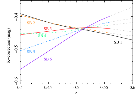
Figure 4: K-corrections computed for the starburst templates of Kinney et al. (1996) and Calzetti, Kinney & Storchi-Bergmann (1994), labelled as in Kinney et al. (1996). K-corrections for templates SB 2–6 are shown as grey dotted lines beyond $z=0.55$ because the templates do not extend below 1250 Å. Template SB 1 has been extended to shorter wavelengths using the spectrum of Mrk 66 from González et al. (1998) to permit K-corrections over the full redshift range.

3.3 Construction of the binned luminosity function

The binned luminosity function was constructed using the method of Page & Carrera (2000). This involves counting the number of galaxies within an absolute magnitude bin and dividing by the four volume of the (volume, absolute-magnitude) space over which the galaxies were counted:

$$\phi_{est}(M)=\frac{N}{\int_{M_{max}}^{M_{min}}\int_{z_{min}}^{z_{max}(M)}\frac{dV}{dz}\,dz\,dM}$$ (2)

where $M$ is absolute magnitude, $\phi_{est}(M)$ is the binned luminosity function, $z$ is redshift and $V$ is volume. $M_{max}$ and $M_{min}$ define the limits of the bin in absolute magnitude, and $z_{max}(M)$ is the maximum redshift to which an object can be detected, or the upper limit of the redshift interval of interest (in our case $z=0.6$), whichever is the smaller. Uncertainties on $\phi_{est}$ were calculated according to Poisson statistics using Gehrels (1986). In order to compute the volume surveyed it is necessary to know the effective sky area surveyed as a function of apparent UVM2 magnitude, which is the product of the completeness and the geometric sky area. (see Section 2.5). The geometric area of our survey is 641 arcmin². For the computation of the binned luminosity function, using the completeness vs apparent magnitude curve (Fig. 3), we have evaluated the effective sky area at a set of discrete apparent magnitudes, given in Table 2.

Table 2: Effective sky area as a function of magnitude, used in the construction of the binned luminosity functions.

UVM2 magnitude	Effective sky area
(mag)	(arcmin2)
20.0	638.8
22.2	624.7
22.4	608.1
22.6	582.4
22.8	561.9
23.0	506.8
23.2	450.4
23.4	382.5
23.5	347.9
23.6	286.4
23.7	219.7
23.8	171.7

3.4 Measuring the Schechter function parameters

We employed a maximum-likelihood fit (Sandage, Tammann & Yahil, 1979) to obtain the best-fitting Schechter-function parameters $\alpha$ and $M^{*}$. We followed the prescription given by Page et al. (2021) to account for photometric uncertainty when carrying out the fit. The approach involves minimising the following expression:

$$C=2N\,ln\left(\int\int\int P(M^{\prime}|M,z)\phi(M)dM\frac{dV}{dz}dM^{\prime}dz\right)$$

$$\ \ \ \ \ \ \ \ \ \ -2\sum^{N}_{i=1}ln\,\int P(M_{i}^{\prime}|M,z_{i})\phi(M_{i})dM$$ (3)

where $C$ is the quantity to be minimised, $z$ is redshift, $\phi$ is the Schechter luminosity function, N is the number of objects in the sample, the subscript $i$ refers to the individual sources and the probability of obtaining a measured absolute magnitude in the interval $M^{\prime}$ to $M^{\prime}+dM^{\prime}$ for a source of true absolute magnitude $M$ is $P(M^{\prime}|M,z)dM^{\prime}$. Uncertainties on the Schechter function parameters $M^{*}$ and $\alpha$ are obtained by varying the parameters until $\Delta C$ reaches significance thresholds equivalent to those commonly applied to $\Delta\chi^{2}$ (Lampton, Margon & Bowyer, 1976). The normalisation $\phi^{*}$ is obtained by setting the model-predicted number of objects in the sample equal to the observed number. For a full explanation/derivation of this approach see Page et al. (2021).

4 Results

The list of positions, redshifts, UVM2 photometry and UVM2-u^∗ colours for galaxies in the redshift range $0.4-0.6$, used to construct and fit the luminosity function, is given in Table 3.

Table 3: UVM2-selected galaxies which were used to construct the luminosity functions. Positions are derived from the UVM2 image. UVM2 mag is the UVM2 apparent magnitude in the AB system. UVM2-u^∗ is the UVM2-u^∗ colour. The column labelled $z$ gives the redshift, and the column labelled spec/phot indicates whether the redshift is derived from spectroscopic or photometric data. Note that only the first five lines are included in the print version. The full table is available electronically.

RA	dec	UVM2 mag	UVM2-u∗	$z$	spec/phot
(J2000)
13 33 36.57	+37 47 03.3	$23.428\pm 0.284$	$0.784\pm 0.285$	0.4508	phot
13 33 36.61	+37 46 39.3	$23.346\pm 0.220$	$0.506\pm 0.220$	0.4948	phot
13 33 36.99	+37 45 18.8	$23.559\pm 0.154$	$0.525\pm 0.156$	0.5188	phot
13 33 37.52	+37 44 00.8	$23.557\pm 0.180$	$0.353\pm 0.182$	0.5995	phot
13 33 37.72	+37 44 43.0	$23.656\pm 0.168$	$0.607\pm 0.169$	0.4223	phot

4.1 Source colours

Figure 5: UVM2 – u^∗ colours against absolute magnitude for the sample of $0.4<z<0.6$ galaxies.

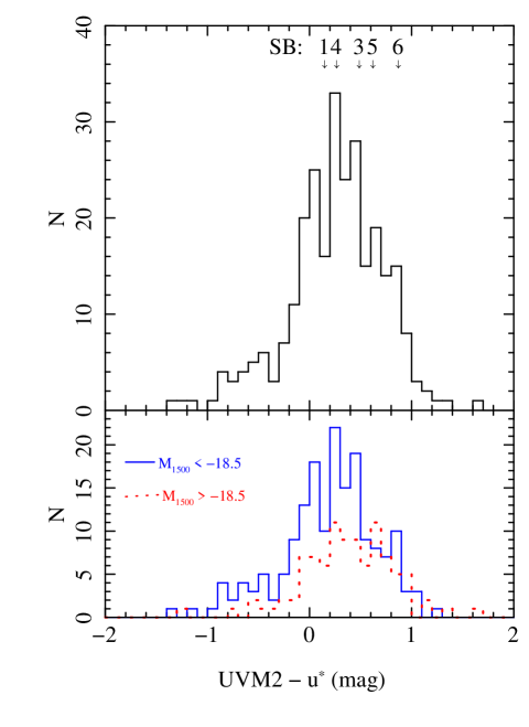
Figure 6: Top panel: distribution of UVM2 – u^∗ colours for the sample of $0.4<z<0.6$ galaxies. At the top the colours of the starburst templates of Kinney et al. (1996) are indicated; SB 2 is not shown because it has almost the same colour as SB 1. Bottom panel: distribution of colours when the sample is split by absolute magnitude.

The UVM2$-$u^∗ colours for our sources are shown against absolute magnitude in Fig. 5. The colours are indicative of the UV spectral shape, which in turn is sensitive to the level of dust attenuation (Meurer, Heckman & Calzetti, 1999), so the colours allow us to assess the typical levels of dust attenuation across the UV luminosity range probed by our survey. The distribution of colours is shown as a histogram in Fig. 6 for the complete sample, and for subsamples split at a threshold absolute magnitude of $M_{1500}=-18.5$. A trend can be seen towards redder colours for the fainter absolute magnitude subsample. The mean colour for the full sample is $\langle$UVM2$-$u${}^{*}\rangle=0.27\pm 0.03$, compared to $\langle$UVM2$-$u${}^{*}\rangle=0.19\pm 0.04$ for the higher luminosity subsample and $\langle$UVM2$-$u${}^{*}\rangle=0.37\pm 0.05$ for the lower luminosity subsample. The means of the two subsamples are different at 3$\sigma$ significance.

4.2 The luminosity function

Table 4: Binned luminosity function measurements. $M_{1500}$ is the centre of the absolute magnitude bin in the rest-frame GALEX FUV band; the absolute magnitude bins are 0.3 mag wide. $\phi$ is the luminosity function. $N$ is the number of galaxies in each bin.

$M_{1500}$	Log $\phi$	$N$
(mag)	(log [Mpc-3 mag-1])
$-20.72$	$-4.57^{+0.52}_{-0.76}$	1
$-20.42$	$-4.27^{+0.37}_{-0.45}$	2
$-20.12$	$-3.97^{+0.25}_{-0.28}$	4
$-19.82$	$-3.66^{+0.17}_{-0.18}$	8
$-19.52$	$-3.15^{+0.09}_{-0.10}$	25
$-19.22$	$-2.97^{+0.08}_{-0.08}$	35
$-18.92$	$-2.76^{+0.07}_{-0.07}$	49
$-18.62$	$-2.61^{+0.05}_{-0.06}$	56
$-18.32$	$-2.42^{+0.06}_{-0.06}$	53
$-18.02$	$-2.35^{+0.09}_{-0.09}$	28
$-17.72$	$-2.13^{+0.14}_{-0.15}$	12

The binned luminosity function with a bin width of 0.3 mag is shown in Fig. 7 and tabulated in Table 4, together with the number of galaxies contributing to each bin. The best-fit values for the Schechter function parameters, with uncertainties considered independently, are $\alpha=-1.8^{+0.4}_{-0.3}$, and $M^{*}=-19.1^{+0.3}_{-0.4}$. The confidence contours for $\alpha$ and $M^{*}$ are shown in Fig. 8; the confidence contours show significant covariance between $\alpha$ and $M^{*}$. The normalisation $\phi^{*}$, obtained as described in Section 3.4 is $3.2\times 10^{-3}$ Mpc^-3. The uncertainty on $\phi^{*}$ has contributions from the Poisson error on the number of objects in the sample, the covariance of $\phi^{*}$ with $\alpha$ and $M^{*}$, and cosmic variance. The Poisson uncertainty amounts to $\pm 2\times 10^{-4}$ Mpc^-3. To derive the uncertainty in $\phi^{*}$ due to its covariance with $\alpha$ and $M^{*}$, we found the upper and lower values of $\phi^{*}$ that correspond to the $\alpha$ and $M^{*}$ values within the 68 percent contour in Fig. 8, which translates to an uncertainty of $+3.9\times 10^{-3}$ Mpc^-3, $-2.2\times 10^{-3}$ Mpc^-3. The contribution from cosmic variance, was assessed to be 15 percent, or $\pm 5\times 10^{-4}$ Mpc^-3, using the online calculator described in Trenti & Stiavelli (2008), assuming completeness and halo filling factors of 0.5, and the Sheth & Tormen (1999) bias prescription. We derive an overall uncertainty for $\phi^{*}$ by adding these three contributions in quadrature, to obtain $\phi^{*}=3.2^{+3.9}_{-2.3}\times 10^{-3}$ Mpc^-3.

Figure 7: UV luminosity function of galaxies in the redshift intervals $0.4<z<0.6$. The datapoints show the binned luminosity function derived from the 13^H field as described in Section 3.3, and the solid curve shows the best-fitting Schechter function derived according to the method described in Section 3.4. For comparison, the dashed lines show the best fitting Schechter function obtained by Arnouts et al. (2005), and the dotted line shows the best-fitting maximum-likelihood Schechter function obtained by Hagen et al. (2015).

Figure 8: Confidence contours for the Schechter function parameters $M^{*}$ and $\alpha$ from the maximum-likelihood fitting. The solid contour corresponds to the 68 per cent confidence region and the dotted contour corresponds to the 95 per cent confidence region. The cross marks the best fit parameter values. The circle and square mark the best fit parameter values found by Arnouts et al. (2005) and Hagen et al. (2015) respectively.

5 Discussion

5.1 The UV colours of UV-selected galaxies

Dust extinction is strong at UV wavelengths, and the degree to which the UV emission from a galaxy is attenuated can be estimated from the shape of its UV continuum (Meurer, Heckman & Calzetti, 1999), or equivalently a UV colour (Seibert et al., 2005). In Page et al. (2021) we showed that the UV colours of our $0.6<z<1.2$, UV-selected galaxies were on average consistent with the lowest-extinction starburst template from the sample of Kinney et al. (1996). The situation is somewhat different for the $0.4<z<0.6$ sample studied here: as seen in Section 4.1, the average UVM2$-$u^∗ colours are different for the most luminous sources ($M_{1500}<-18.5$) and the less luminous sources ($M_{1500}>-18.5$) in our sample. For context, a UVM2$-$u^∗ colour of $-0.5$ corresponds to a spectral slope $\beta=-2.9$, and UVM2$-$u${}^{*}=1$ corresponds to $\beta=-0.1$; 90 percent of our galaxies lie within the range delimited by these two colours. To facilitate comparison with the Kinney et al. (1996) templates, we have labelled the positions of colours derived from the templates at $z=0.5$ on the top panel of Fig. 6. The template colours change little over the redshift interval $0.4<z<0.6$: up to $\pm 0.03$ for SB 1$-$SB 4 and up to $\pm 0.07$ for SB 5 and SB 6. The mean colour of the luminous subsample ($\langle$UVM2$-$u${}^{*}\rangle=0.19\pm 0.04$) is consistent with the expected colour (UVM2$-$u^∗=0.15) of the lowest-extinction template, SB 1. The luminosity ranges probed by Page et al. (2021) at $0.6<z<1.2$ do not reach as low as $M_{1500}=-18.5$, in absolute terms, or relative to $M^{*}$ at the respective redshifts, so could be considered equivalent to our luminous subsample. Hence in this regard we find a consistent picture to that found at higher redshift by Page et al. (2021), that the most luminous UV-selected galaxies have UV colours consistent with very low levels of extinction.

At the lower luminosities probed by our $0.4<z<0.6$ sample ($M_{1500}>-18.5$), the mean colour ($\langle$UVM2$-$u${}^{*}\rangle=0.37\pm 0.05$) lies between the colours expected from templates SB 3 (UVM2$-$u^∗=0.49) and SB 4 (UVM2$-$u^∗=0.27) indicating an increased level of average extinction. We note that a similar pattern is seen in the UV spectral index measurements of UV-selected galaxies at $z\sim 1.5$ in the study of Heinis et al. (2013); in their fig. 5 the mean spectral index $\beta$ is practically constant for all except the lowest two luminosity bins, which correspond to $M_{1500}>-18.4$, or $M_{1500}>M^{*}+1$, in which the slope becomes redder. The change in mean UVM2$-$u^∗ colour between our higher and lower luminosity subsamples corresponds to a change in spectral index $\beta$ of 0.3, similar to that observed by Heinis et al. (2013). However, in other studies focused at higher redshifts ($1<z<8$) the opposite trend (i.e. more luminous galaxies have redder UV slopes than less luminous galaxies) has been observed (Wilkins et al., 2011; Bouwens et al., 2014; Kurczynski et al., 2014).

The appearance of sources with higher levels of extinction at absolute magnitudes somewhat fainter than $M^{*}$ is a natural expectation if the luminosity distribution is similar for sources with and without extinction, given the steepness of the Schechter function shape at the bright end. Extinction will push the contribution of sources to fainter UV absolute magnitudes, but the luminosity function rises so quickly at the bright end as luminosity decreases that the contribution of luminous sources with any significant extinction will be easily overwhelmed in numerical terms by lower-luminosity, low-extinction galaxies. Fainter than $M^{*}$, however, the luminosity function is less steep, and it becomes possible for sources pushed to lower absolute magnitude by extinction to contribute.

Note that despite the small change in average colour towards fainter absolute magnitude we have retained the K-corrections based on template SB 1 for all galaxies in the sample. While diagnostic of the overall spectral shape, we do not consider UVM2$-$u^∗ to be a reliable predictor of the spectral shape at $1,500$ Å to the extent that we should K-correct the luminosities on an individual basis. The difference in K-corrections between SB 1 and SB 3 or SB 4 amounts to only a few hundredths of a magnitude for most of the galaxies in our sample.

5.2 The UV luminosity function of galaxies

Moving now to the luminosity function, we note that our survey is based on a slightly larger sample of objects than that of Arnouts et al. (2005) for the same redshift range. Our binned luminosity function (Fig. 7) shows less scatter in $\phi$ at the bright end than that of Arnouts et al. (2005, their Fig. 2) but their survey probes absolute magnitudes about 0.5 mag fainter than ours. Compared to the survey of Hagen et al. (2015), again our survey contains slightly more objects in the redshift range $0.4<z<0.6$; our faint absolute magnitude limit is similar to the completeness limit adopted by Hagen et al. (2015) in this redshift range. The survey of Bhattacharya, Saha & Mondal (2023), in contrast, probes absolute magnitudes about two magnitudes fainter than our survey, and contains twice as many objects in the redshift range $0.4<z<0.6$, but covers only a quarter of the sky area.

Comparing our binned luminosity function (see Fig. 7) with the best-fit Schechter functions of Arnouts et al. (2005) and Hagen et al. (2015), our luminosity function falls below their Schechter function models at the brightest absolute magnitudes and above their models at the faintest absolute magnitudes. Inspection of fig. 2 of Arnouts et al. (2005) and table 3 of Hagen et al. (2015) confirms that these differences are seen directly in the binned functions as well as in the models. Given these differences between their binned luminosity functions and ours, it is unsurprising that their best fit models are not compatible with ours. Comparing their best-fit values of $\alpha$ and $M^{*}$ with the confidence intervals we derive on these parameters (Fig. 8), we see that they are well outside our 95 percent confidence interval. The $\Delta C$ corresponding to their best fits (see Section 3.4) indicates that the best-fitting model of Arnouts et al. (2005) is excluded by our data at 4$\sigma$ significance, and that of Hagen et al. (2015) at $>5\sigma$. For $\alpha=-1.55$, as found by Arnouts et al. (2005) and assumed by Hagen et al. (2015) in this redshift range, our fitting would suggest $M^{*}=-18.9\pm 0.1$, 0.5–0.8 magnitudes fainter than found in those studies.

That we find a fainter value of $M^{*}$ than Arnouts et al. (2005) or Hagen et al. (2015) in the redshift range 0.4–0.6 (see Fig. 9) forms a consistent pattern with the XMM-OM-derived results of Page et al. (2021), Sharma, Page & Breeveld (2022) and Sharma et al. (2024) at redshifts of 0.6–1.2. Those papers attributed the difference to the careful purging of AGN contamination in the studies based on XMM-OM. We can investigate the issue in our lower redshift study by considering what would happen to our luminosity function if we put back the two AGN that were excluded in Section 2.7. Despite this very small number of broad-line AGN, one of them has an absolute magnitude $M_{1500}=-21.25$, and would thus be the most luminous object in the sample. Repeating the maximum likelihood fitting, with these two AGN included, shifts the best-fit value of $M^{*}$ to -19.7, consistent with the $M^{*}$ values found by Arnouts et al. (2005) and Hagen et al. (2015). We thus consider that in this study also, the different treatment of AGN can explain the discrepancy in $M^{*}$ with the values found by Arnouts et al. (2005) and Hagen et al. (2015).

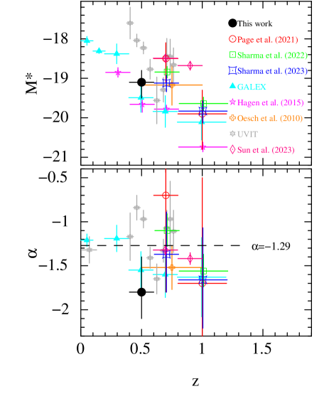
Figure 9: Direct UV measurements of Schechter function parameters $M^{*}$ and $\alpha$ over the redshift interval $0<z<1.2$. The points labelled ‘GALEX’ correspond to the measurements of Wyder et al. (2005) for $z<0.1$, Treyer et al. (2005) for $0.1<z<0.2$ and Arnouts et al. (2005) for $z>0.2$. The points labelled ‘UVIT’ correspond to the measurements of Bhattacharya, Saha & Mondal (2023). The dashed line in the lower panel shows the result of fitting a single value to all measurements of $\alpha$ out to $z=1.2$.

Fig. 9 shows the direct measurements of the Schechter function parameters $M^{*}$ and $\alpha$ out to $z=1$ from space-based UV data in the literature as well as from this study. A robust trend of $M^{*}$ brightening with increasing redshift can be seen in the top panel of Fig. 9, despite the scatter in $M^{*}$ values between different studies and the large variation of $M^{*}$ within the study of Bhattacharya, Saha & Mondal (2023).

For the faint-end slope $\alpha$, if we set aside Bhattacharya, Saha & Mondal (2023), our measurement is one of only two covering the redshift range $0.4<z<0.6$; our measurement is fully consistent with the other measurement covering this redshift range, which comes from Arnouts et al. (2005). Bhattacharya, Saha & Mondal (2023) utilised narrow redshift shells to construct their luminosity functions, and have four separate measurements of $\alpha$ which overlap the $0.4<z<0.6$ range. Taking the weighted average of those four measurements gives $\alpha=-1.10\pm 0.07$, flatter than our measurement or that of Arnouts et al. (2005), but consistent with both at 2$\sigma$. Overall, there is little sign of any trend between $\alpha$ and $z$ in Fig. 9. Fitting a single constant value to the measurements of $\alpha$ out to $z=1.2$, shown in Fig. 9 yields a best fit of $\alpha=-$1.29$\pm 0.03$ and a $\chi^{2}$ value of 44.3 for 24 degrees of freedom, an acceptable fit with a null-hypothesis probability of 0.01. On this basis we therefore consider that the present measurements are consistent with an unchanging $\alpha=-$1.29$\pm 0.03$ over the whole redshift range $z=0$ to $z=1.2$. For a fixed $\alpha=-1.29$, our maximum-likelihood fitting to the 13^H field data for $0.4<z<0.6$ would yield $M^{*}=-18.7\pm 0.1$.

In contemporary models for the galaxy population, the faint end slope $\alpha$ of the galaxy luminosity function is primarily determined by the physics of feedback from star-formation, particularly in driving gaseous outflows (Benson et al., 2003; Bower, Benson & Crain, 2012; Somerville & Davé, 2015). An unchanging (or little changing) faint-end slope since $z=1.2$ would imply that the processes that regulate star formation in low-mass galaxies have produced the same power-law distribution of star formation rates for more than half of the Universe’s history despite the large changes in overall star-formation rate, metallicity, and large-scale baryon disposition that have occurred during that time. Such a robust faint-end slope would be all the more intriguing given the measurements of a much steeper faint-end slope at earlier cosmic epochs (e.g. Parsa et al., 2016; McLeod et al.,, 2024).

It is interesting to consider our findings on $\alpha$ in the context of two works which examine the UV luminosity function in this redshift range, but are not shown in Fig. 9 because the UV measurements are extrapolated from longer wavelengths. Cucciati et al. (2012) estimated rest-frame UV magnitudes through spectral energy distribution model fits to deep multi-band optical and near-IR photometry for a sample of more than 7,000 galaxies with spectroscopic redshifts. Taking the weighted average of their estimates for $\alpha$ over the redshift interval $0<z<1.2$ yields $\alpha=-1.05\pm 0.03$, flatter than the faint-end slope $\alpha=-1.29\pm 0.03$ derived directly from UV surveys, and inconsistent at 6$\sigma$ significance.

Moutard et al. (2020) also estimated rest-frame UV magnitudes through spectral energy distribution fits to multi-band photometry, but using more than a million galaxies, and predominantly with photometric redshifts. They included GALEX photometry in their multi-band fitting for some of their sources, so their luminosity functions are based on a mixture of direct UV measurements and extrapolations. Moutard et al. (2020) find that their fitted values of $\alpha$ vary little with redshift. In the redshift range $0<z<1.3$ the weighted mean of their fitted values is $\alpha=-1.39\pm 0.01$. This value, in contrast to that of Cucciati et al. (2012), is steeper than $\alpha=-1.29\pm 0.03$ derived directly from UV surveys, and inconsistent at 3$\sigma$ significance. Therefore in terms of the faint-end slope $\alpha$, neither Cucciati et al. (2012) nor Moutard et al. (2020) can be reconciled with the present ensemble of direct measurements from UV surveys, though the discrepancy is smaller for the measurements of Moutard et al. (2020).

6 Conclusions

We have used UVM2 imaging of the 13^H extragalactic survey field, obtained with XMM-OM and Swift UVOT to study the UV colours and rest-frame 1,500 Å luminosity function of galaxies in the redshift range $0.4<z<0.6$.

Our luminosity function is constructed from a slightly larger sample of galaxies than either of the comparable preceding GALEX and Swift studies (Arnouts et al., 2005; Hagen et al., 2015) in this redshift range, and covers a larger sky area than the Astrosat UVIT study of Bhattacharya, Saha & Mondal (2023). We obtain a best-fitting Schechter function faint-end slope $\alpha=-1.8^{+0.4}_{-0.3}$, steeper but consistent with the two previous direct determinations in this redshift range (Arnouts et al., 2005; Bhattacharya, Saha & Mondal, 2023). Combining our measurement of $\alpha$ with previous $z<1.2$ measurements from space-borne UV data, we find little evidence for any trend with redshift, with the ensemble of measurements showing consistency with $\alpha=-1.27\pm 0.03$ at all redshifts to $z=1.2$. Our best-fitting characteristic magnitude $M^{*}$ is $-19.1^{+0.3}_{-0.4}$, fainter than that found in the previous studies of Arnouts et al. (2005) and Hagen et al. (2015). We find that contamination of our UV-selected sample by AGN, while small in number, would have led to more luminous $M^{*}$ if the AGN had not been removed from the sample. In this regard our results are in keeping with our XMM-OM based studies at higher redshift, which also found fainter values of $M^{*}$ than previous studies, and in which we have shown that careful purging of AGN contamination is essential for the determination of $M^{*}$.

We find that the average UV colour of the most luminous UV galaxies ($M_{1500}<-18.5$) is consistent with the lowest-extinction ($E_{B-V}<0.1$) starburst template from the ensemble of Kinney et al. (1996), implying that the bright end of the UV luminosity function is dominated by galaxies with low levels of dust attenuation. For absolute magnitudes fainter than $M_{1500}=-18.5$ the average UV colour is redder, characteristic of starburst templates with higher extinction ($E_{B-V}$ between 0.25 and 0.50), suggesting that more dust-attenuated galaxies only start to contribute significantly to the UV luminosity function at absolute magnitudes fainter than $M^{*}$.

7 Data Availability

The primary data underlying this article are available from the XMM-Newton Science archive at https://www.cosmos.esa.int/web/xmm-newton, and the Swift Science data archives at https://www.swift.ac.uk and https://swift.gsfc.nasa.gov. Supplementary data underlying this article will be shared on reasonable request to the corresponding author.

APPENDIX A: Relative throughput of XMM-OM and Swift UVOT employing the UVM2 filter

In order to use a combined UVOT and XMM-OM image to generate our catalogue of UVM2-selected galaxies, the count rates in the data from one of the instruments must be scaled so that a source of a given UVM2 magnitude will correspond to the same count rate in both instruments. We have implimented this adjustment by scaling the XMM-OM exposure map. The scaling is based on the difference in zeropoints for the two instruments, but also must take into account the different aperture corrections that relate the instrumental zeropoints to the measurement aperture employed in the source-searching and measurement software (in our case, omdetect). The scaling must also account for colour terms that arise from the small difference in the shapes of the UVM2 passband between the two instruments. We will describe each of these components in turn.

APPENDIX A.1 instrumental zeropoints

The AB zeropoint for XMM-OM in the UVM2 filter is 17.412, for a 17.5 arcsec radius aperture (Rosen et al., 2023). The AB zeropoint for Swift UVOT in the UVM2 filter is 18.54, for a 5 arcsec radius aperture (Breeveld et al., 2011).

APPENDIX A.2 aperture corrections

The photometric measurements in our UVM2 source catalogue are obtained from the software omdetect. Almost all galaxies at $0.4<z<0.6$ are indistinguishable from point sources at the spatial resolution and depth of our UVM2 image. For faint, point-like sources, omdetect employs a circular aperture of radius 2.8 arcsec to measure photometry (Page et al., 2012), hence for both XMM-OM and UVOT the different aperture corrections from the aperture for which their instrumental zeropoint is defined to the 2.8 arcsec radius measurement aperture must be taken into account.

The XMM-OM has a stable PSF thanks to its carefully controlled thermal environment. The aperture correction from the 17.5 arcsec aperture that corresponds to the instrumental zeropoint to a 2.8 arcsec aperture is therefore obtained from the XMM-Newton Current Calibration Files. This aperture correction is 0.278 magnitudes.

On the other hand, the PSF of the UVOT shows small variations as the thermal environment of the telescope changes over Swift’s 90 minute orbit. Hence aperture corrections for UVOT are best measured directly from the UVOT images on which they will be employed (Poole et al., 2008; Breeveld et al., 2010). Therefore we measured aperture corrections from nine stars of appropriate magnitude in the UVOT image by obtaining, for each star, photometry in 5 arcsec and 2.8 arcsec apertures using the Swift FTOOL uvotsource. For each star the difference between the magnitudes obtained in the two apertures represents a measurement of the aperture correction. These measurements were then averaged to obtain a mean aperture correction of $0.249\pm 0.007$ magnitudes from a 5 arcsec radius aperture (for which the instrumental zeropoint is defined) to the 2.8 arcsec measurement aperture.

The difference between the XMM-OM and UVOT aperture corrections is 0.029 magnitudes.

APPENDIX A.3 colour correction

As seen in Fig. 1, the shapes of the UVM2 bandpass are similar but not identical for XMM-OM and UVOT. Therefore in comparing the photometric responses of the two instruments, there is a small colour term to consider, which will depend on the spectrum of the source being observed. We have synthesized these colour terms for the six template galaxy spectra which were used to investigate the K-correction in Section 3.2. The colour term can be expressed as UVM2${}_{\rm XMM-OM}-$UVM2_UVOT where UVM2_XMM-OM is the magnitude of an object in the UVM2 bandpass of XMM-OM and UVM2_UVOT is the magnitude of an object in the UVM2 bandpass of UVOT. The colour terms range from $-0.01$, $-0.02$ and $-0.04$ magnitudes for the lowest extinction SB 1, SB 2, and SB 3 templates respectively at $z=0.4$ to $-0.06$, $-0.06$ and $-0.08$ magnitudes for the highest extinction SB 4, SB 5 and SB 6 templates at $z=0.5$, with the variation of colour with redshift contributing up to 0.02 magnitudes. Given that our sample is dominated by low extinction sources (see Section 4.1) we consider that a typical colour term is UVM2${}_{\rm XMM-OM}-$UVM2${}_{\rm UVOT}=-0.03$.

APPENDIX A.3 overall throughput adjustment

The difference in instrumental UVM2 zeropoints between XMM-OM and Swift UVOT is 1.128 mag. To this we should add an aperture correction of 0.029 mag and a colour correction of $-0.03$ magnitudes, but as the aperture and colour corrections almost perfectly cancel, we have simply adopted the difference in the instrumental zeropoints to represent the throughput difference.

APPENDIX A.4 systematic errors

It is important to consider the degree of systematic error we may be introducing by combining the XMM-OM and UVOT images.

The systematic uncertainty on the instrumental zeropoint (i.e. the uncertainty on global photometry) for Swift UVOT is reckoned to be 0.03 mag (Poole et al., 2008). There is no equivalent number in the calibration documentation for XMM-OM, but as the two instruments are calibrated against overlapping sets of photometric standard stars, we expect any error in the zeropoint of UVOT to be replicated systematically in the XMM-OM zeropoint. Hence we would expect the zeropoint uncertainty of 0.03 mag to apply similarly to the combination of XMM-OM and UVOT data.

Uncertainties arising from the aperture corrections would be expected to be dominated by the uncertainty on the UVOT aperture correction, i.e. 0.007 mag. Uncertainties related to colour correction, given the spread in corrections for different galaxy templates, could amount to as much as 0.03 mag, much larger than the uncertainty due to aperture effects. The quadrature sum of the uncertaintes from aperture and colour corrections is 0.03 mag, similar to the level of systematic uncertainty on the zeropoints of the two instruments.

For our study of faint galaxies, we have taken a signal to noise threshold of 4. This corresponds to a statistical photometric uncertainty of 0.3 mag. This statistical uncertainty is around ten times larger than the systematic uncertainty that might be contributed by combining XMM-OM and UVOT data, and hence our photometric uncertainty is dominated by statistical, rather than systematic, uncertainty.

References

- Adelman-McCarthy et al. (2008) Adelman-McCarthy J.K., et al., 2008, ApJS, 175, 297
- Arnouts et al. (2005) Arnouts S., et al., 2005, ApJ, 619, L43
- Benson et al. (2003) Benson A.J., Bower R.G., Frenk C.S., Lacey C.G., Baugh C.M., Cole S., 2003, ApJ. 599, 38
- Bhattacharya, Saha & Mondal (2023) Bhattacharya S., Saha K., & Mondal C., 2023, arXiv:2310.01903v1
- Bolzonella et al. (2000) Bolzonella M., Miralles J.-M., Pelló R., 2000, A&A, 363, 476
- Bower, Benson & Crain (2012) Bower R.G., Benson A.J., Crain R.A., 2012, MNRAS, 422, 2816
- Bouwens et al. (2009) Bouwens R.J., et al., 2009, ApJ, 705, 936
- Bouwens et al. (2014) Bouwens R.J., et al., 2014, ApJ, 793, 115
- Bouwens et al. (2021) Bouwens R.J., et al., 2021, AJ, 162, 47
- Breeveld et al. (2010) Breeveld A.A., et al., 2010, MNRAS, 406, 1687
- Breeveld et al. (2011) Breeveld A.A., Landsman W., Holland S.T., Roming P., Kuin N.P.M., Page M.J., 2011, AIP Conference Proceedings 1358, 373
- Branduardi-Raymont et al. (1994) Branduardi-Raymont G., et al., 1994, MNRAS, 270, 947
- Calzetti, Kinney & Storchi-Bergmann (1994) Calzitti D., Kinney A.L., Storchi-Bergmann T., 1994, ApJ, 429, 582
- Cucciati et al. (2012) Cucciati O., et al., 2012, A&A, 539, A31
- Donnan et al. (2023) Donnan C.T., et al., 2023, MNRAS, 518, 6011
- Fordham, Moorhead & Galbraith (2000) Fordham J. L. A., Moorhead C. F., Galbraith R. F., 2000, MNRAS, 312, 83
- Gehrels (1986) Gehrels N., 1986, ApJ, 303, 336
- González et al. (1998) González R.M., Leitherer C., Heckman T., Lowenthal J.D., Ferguson H.C., Robert C., 1998, ApJ, 495, 698
- Hagen et al. (2015) Hagen L.M.Z., Hoversten E.A., Gronwall C., Wolf C., Siegel M.H., Page M., Hagen A., 2015, ApJ, 808, 178
- Harikane et al. (2023) Harikane Y., et al., 2023, ApJS, 265, 5
- Heinis et al. (2013) Heinis, S., et al., 2013, MNRAS, 429, 1113
- Kennicutt & Evans (2012) Kennicutt R.C. & Evans N.J., 2012, ARA&A, 50, 531
- Kinney et al. (1996) Kinney A.L., Calzetti D., Bohlin R.C., McQuade K., Storchi-Bergmann T., Schmitt H.R., 1996, ApJ, 467, 38
- Kurczynski et al. (2014) Kurczynski P., et al., 2014, ApJ, 793, L5
- Kuin & Rosen (2008) Kuin N.P.M. & Rosen S.R., 2008, MNRAS, 383, 383
- Lampton, Margon & Bowyer (1976) Lampton M., Margon B., Bowyer S., 1976, ApJ, 208, 177
- Loaring et al. (2005) Loaring N.S., et al., 2005, MNRAS, 362, 1371
- Madau et al. (1996) Madau P., Ferguson H.C., Dickinson M.E., Giavalisco M., Steidel C.C., Fruchter A., 1996, MNRAS, 283, 1388
- Martin et al. (2005) Martin D.C., et al., 2005, ApJ, 619, L1
- Mason et al. (2001) Mason K. O., et al., 2001, A&A, 365, L36
- McLeod et al., (2024) McLeod D.J., et al., 2024, MNRAS, 527, 5004
- McHardy et al. (1998) McHardy I.M., et al., 1998, MNRAS, 295, 641
- McHardy et al. (2003) McHardy I.M., et al., 2003, MNRAS, 342, 802
- Meurer, Heckman & Calzetti (1999) Meurer G.R., Heckman T.M. & Calzetti D., 1999, ApJ, 521, 64
- Moutard et al. (2020) Moutard T., Sawicki M., Arnouts S., Golob A., Coupon J., Ilbert O., Yang X., Gwyn S., 2020, MNRAS, 494, 1894
- Oesch et. al. (2010) Oesch P.A., et al., 2010, ApJ, 725, L150
- Oke & Gunn (1983) Oke J. B., Gunn J. E., 1983, ApJ, 266, 713
- Page & Carrera (2000) Page M.J., Carrera F.J., 2000, MNRAS, 311, 433
- Page et al. (2006) Page M.J., et al., 2006, MNRAS, 369, 156
- Page et al. (2012) Page M.J., et al., 2012, MNRAS, 426, 903
- Page et al. (2013) Page M.J., et al., 2013, MNRAS, 436, 1684
- Page et al. (2017) Page M.J., et al., 2017, MNRAS, 466, 1061
- Page et al. (2021) Page M.J., et al., 2021, MNRAS, 506, 473
- Parsa et al. (2016) Parsa S., Dunlop J.S., McLure R.J., Mortlock A., 2016, MNRAS, 456, 3194
- Pérez-González et al. (2023) Pérez-González P.G., et al., 2023, arXiv:2302.02429
- Poole et al. (2008) Poole T.S., et al., 2008, MNRAS, 383, 627
- Reddy & Steidel (2009) Reddy N.A., Steidel C.C., 2009, ApJ, 692, 778
- Roming et al. (2005) Roming P.W.A., et al., 2005, Space Sci. Rev., 120, 95
- Rowan-Robinson et al. (2008) Rowan-Robinson M., et al., 2008, MNRAS, 386, 697
- Rosen et al. (2023) Rosen S. & OMCal Team, 2023, XMM-SOC-CAL-TN-0019 Issue 8.0, available from https://www.cosmos.esa.int/web/xmm-newton/calibration-documentation
- Sandage, Tammann & Yahil (1979) Sandage A., Tammann G.A., Yahil A., 1979, ApJ, 232, 352
- Schlafly & Finkbeiner (2011) Schlafly E.F., Finkbeiner D.P., 2011, ApJ, 737, 103
- Schechter (1976) Schechter P., 1976, ApJ, 203, 297
- Schlegel, Finkbeiner & Davis (1998) Schlegel D.J., Finkbeiner D.P., Davis M., 1998, ApJ, 500, 525
- Seymour, McHardy & Gunn (2004) Seymour N., McHardy I.M. & Gunn K.F., 2004, MNRAS, 352, 131
- Sharma, Page & Breeveld (2022) Sharma M., Page M.J. & Breeveld A.A., 2022, MNRAS, 511, 4882
- Sharma et al. (2024) Sharma M., Page M.J., Ferreras I., Breeveld A.A., 2024, MNRAS, 531, 2040
- Sheth & Tormen (1999) Sheth R.K., & Tormen G., 1999, MNRAS, 308, 119
- Seibert et al. (2005) Seibert M., et al., 2005, ApJ, 619, L55
- Somerville & Davé (2015) Somerville R.S. & Davé R., 2015, ARA&A, 53, 51
- Steidel et al. (2006) Steidel C.C., Giavalisco M., Pettini M., Dickinson M., Adelberger K.L., 2006, ApJ, 462, L17
- Sullivan et al. (2000) Sullivan M., Treyer M.A., Ellis R.S., Bridges T.J., Milliard B., Donas J., 2000, MNRAS, 312, 442
- Sun et al. (2023) Sun L., et al., 2023, arXiv:2311.15664v1
- Tandon et al. (2017) Tandon S.N., et al., 2017, JApA, 38, 28
- Trenti & Stiavelli (2008) Trenti M., & Stiavelli M., 2008, ApJ, 676, 767
- Treyer et al. (1998) Treyer M.A., Ellis R.S., Milliard B., Donas J., Bridges T.J., 1998, MNRAS, 300, 303
- Treyer et al. (2005) Treyer M., et al., 2005, ApJ, 619, L19
- Wilkins et al. (2011) Wilkins S.M., Bunker A.J., Stanway E., Lorenzoni S., Caruana J., 2011, MNRAS, 417, 717
- Wyder et al. (2005) Wyder T.K., et al., 2005, ApJ, 619, L15
- Xu et al. (2005) Xu C.K., et al., 2005, ApJ, 619, L11