22institutetext: Faculty of Mathematics and Computer Science, A. Mickiewicz University, Uniwersytetu Poznańskiego 4, 61-614 Poznań, Poland
Ultraluminous X-ray sources in Globular Clusters
This paper investigates the formation, populations, and evolutionary paths of UltraLuminous X-ray Sources (ULXs) within Globular Clusters (GCs). ULXs, characterised by their extreme X-ray luminosities, present a challenge to our understanding of accretion physics and compact object formation. While previous studies have largely focused on field populations, this research examines the unique environment of GCs, where dynamical interactions play a significant role. Using the MOCCA Monte Carlo code, we explore how dynamics influences ULX populations within these dense stellar clusters.
Our findings reveal that dynamical processes, such as binary hardening and exchanges, can both facilitate and impede ULX formation in GCs. The study explores the impact of parameters including the initial binary fraction, tidal filling, and multiple stellar populations on the evolution of ULXs. We find that non-tidally filling clusters exhibit significantly larger ULX populations compared to tidally filling ones.
The results indicate that the apparent scarcity of ULXs in GCs may be related to the older stellar populations of GCs relative to the field. Furthermore, the study identifies a population of ”escaper” ULXs, which originate in GCs but are ejected and emit X-rays outside the cluster. These escapers may significantly contribute to the observed field ULX population.
Key Words.:
stellar dynamics – methods: numerical – globular clusters: evolution – X-ray: binaries1 Introduction
Ultraluminous X-ray sources (ULXs) have been a subject of intense study in the field of high-energy astrophysics for several decades. These enigmatic objects, characterized by X-ray luminosities exceeding , challenge our understanding of accretion physics and compact object formation (see e.g. Kaaret et al. 2017a, b, for a recent review). With over known ULXs identified to date (Walton et al. 2022), they represent a significant population of extreme X-ray emitters in the Universe, yet their fundamental nature remains a topic of ongoing debate.
The diversity of ULXs has been highlighted in recent classification schemes (e.g. Wiktorowicz et al. 2017), which attempt to categorize these objects based on their observational properties and potential underlying physical mechanisms. While the majority of ULXs were initially thought to harbor intermediate-mass black holes (IMBHs), our understanding has evolved considerably with the detection of pulsar accretors (Bachetti et al. 2014).
The importance of studying ULXs, particularly in the context of globular clusters (GC), cannot be overstated. These objects serve as laboratories for extreme accretion physics, potentially shedding light on the formation and evolution of double compact objects (DCOs) - the progenitors of gravitational wave sources. Moreover, ULXs continue to be considered as candidates for elusive IMBHs (Kaaret et al. 2017a, and references therein).
A critical aspect of ULX research involves identifying and characterizing their donor stars. Heida et al. (2016); López et al. (2020) reported that some ULXs had been identified with potential red super-gian (RSG) donors using infrared spectroscopy data. They examined a total of ULXs using photometric techniques in the infrared band, resulting in the identification of candidate counterparts for objects. Among these, the nature of sources was confirmed through spectroscopic analysis, with only five categorized as ULXs likely to have RSG donors.
In this paper, we present a comprehensive study of ULXs in globular clusters, focusing on their stellar-mass manifestations. The dense stellar environment introduces additional complexities and possibilities for exotic binary formations. By examining their properties, distribution, and potential formation mechanisms, we aim to contribute to the broader understanding of ULX physics and their role in compact object evolution.
1.1 Globular Cluster environment
GCs are dense, quasi-spherical collections of stars that orbit the centers of galaxies. These typically old stellar systems, often containing millions of stars within a relatively small volume, are hubs of dynamical interactions. Their evolution is governed by the relaxation process connected with continuous distance gravitational interactions between all objects in the cluster.
This leads to global phenomena like, core collapse, i.e. contraction of the cluster core and gradual increase in central density, and mass segregation, i.e. the tendency of heavier stars to occupy the central regions, while pushing the lighter stars outwards. Close dynamical interactions influence also the stars and binaries individually, influencing the binary parameters (e.g. the separation and eccentricity), or through exchanges (e.g. binary changes one of it’s component into another star), ejections (star or binary becomes unbound with the cluster), and binary formation (single stars became bound and form a binary). Such dynamical encounters in dense star clusters can also lead to the formation of close binary systems, including X-ray binaries (Pooley et al. 2003; Ivanova et al. 2005, 2008). Understanding how the fundamental dynamics influence the ULX formation is essential for interpreting the presence and characteristics of these exotic objects in GC environments.
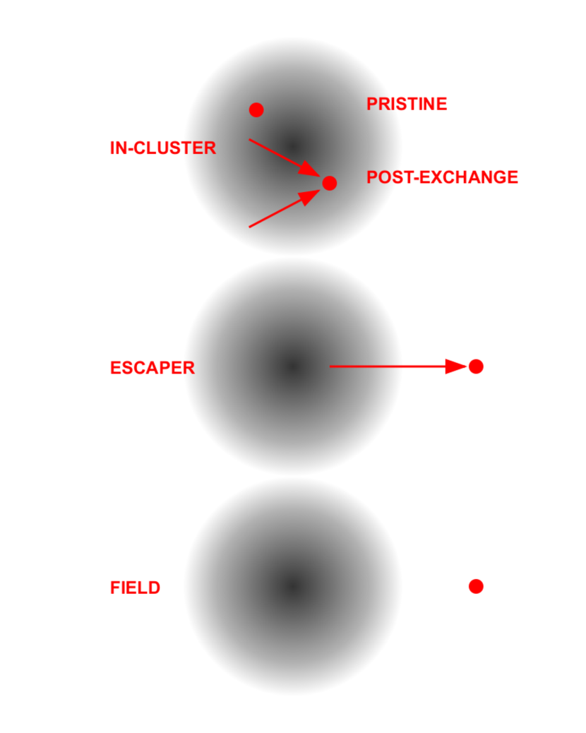
Figure 1 illustrates three pathways for ULX formation in relation to GCs. In the ”IN-CLUSTER” scenario, ULX progenitors form and remain bound to the cluster, often through multiple dynamical interactions, including exchanges. ”ESCAPER” ULXs originate in the GC but are ejected through interactions, emitting outside the cluster while retaining their GC-imprinted dynamical history. ”FIELD” ULXs, by contrast, form and evolve in isolation. The key distinction lies in the dynamical imprint: ”ESCAPER” ULXs bear the hallmarks of GC interactions, unlike ”FIELD” systems, which provide a baseline for understanding the unique contribution of clusters to ULX formation.
1.2 GCULX candidates
While the majority of ULXs are detected in star-forming regions of galaxies, there is increasing evidence for their presence in GCs as well. Pioneering observations of GCULXs have been reported in several galaxies, with varied GC environments, spectral behavior, and variability patterns.
Maccarone et al. (2007) discovered the first ULX in a GC (NGC 4472). It exhibits an X-ray luminosity of and rapid variability. Similar detections were reported in NGC 1399 (Shih et al. 2010; Irwin et al. 2010), with more GCULXs in NGC 4472 (Maccarone et al. 2011) and NGC 4649 (Roberts et al. 2012). Some sources identified in GCs exhibited flares just above the ULX-defining limit of (Irwin et al. 2016; Sivakoff et al. 2005).
Recent observations have extended the known GCULX population, including seven additional GCULXs associated with M87 GCs (Dage et al. 2020), three in NGC 1316 (Dage et al. 2021), and new candidates in GCs of massive () early-type galaxies (Thygesen et al. 2023).
In dense stellar systems, compact objects can be readily ejected, which can considerably impact the formation channels of such objects (e.g. Kulkarni et al. 1993). Furthermore, GCs typically exhibit high ages and, consequently, fewer higher-mass stars. These characteristics contribute to the intriguing nature of GCULXs.
2 Methodology
2.1 MOCCA Monte Carlo Code
The MOCCA (MOnte Carlo Cluster evolution Code; Hypki & Giersz 2013) is a state-of-the-art numerical tool that combines the Monte Carlo method for stellar dynamics (Hénon 1971; Stodolkiewicz 1986) with detailed stellar and binary evolution algorithms from the BSE code (Hurley et al. 2000, 2002) with recent updates (level-C from Kamlah et al. 2022, and references therein) and low-N scattering code FEWBODY (Fregeau et al. 2004) to follow close dynamical interactions. This hybrid approach makes MOCCA particularly well-suited for studying the formation and evolution of exotic objects like ULXs in dense stellar environments, offering an optimal balance between computational efficiency and physical accuracy.
Recent improvements to the MOCCA code (Hypki et al. 2022, 2025; Giersz et al. 2024) have significantly enhanced its capabilities for ULX studies. First of all, the mass transfer calculations now incorporate a more sophisticated treatment of super-Eddington accretion, crucial for modeling ULX systems (Shakura & Sunyaev 1973; Wiktorowicz et al. 2015). Additionally, improvements in core radii calculations improved the RLOF calculations. The introduction of detailed evolutionary tracking provide unprecedented insight into the spatial distribution and evolutionary pathways of ULX systems within clusters equivalent to detailed outputs from codes like startrack (Belczynski et al. 2008).
A major advancement relevant to this study is MOCCA’s capability to handle multiple stellar populations (MSPs), a phenomenon now recognized as ubiquitous in globular clusters (e.g. Piotto et al. 2015; Renzini et al. 2015; Gratton et al. 2019; Bastian & Lardo 2018; Milone & Marino 2022). While a comprehensive analysis of MSPs in our models is presented in Hypki et al. (2022, 2025); Giersz et al. (2024), here we specifically investigate their impact on ULX formation and evolution. The code now tracks different stellar populations with distinct chemical compositions, ages, and spatial distributions, allowing us to examine how MSP-specific properties affect compact object formation and ULX characteristics.
All recent changes to the MOCCA code are described in details in Giersz et al. (2024).
2.2 Simulations
The MOCCA code employs hundreds of parameters to govern the dynamical and stellar evolution of globular clusters. Based on previous studies of compact object populations - including cataclysmic variables (Belloni et al. 2017), ULXs in the field (Wiktorowicz et al. 2019), and double white dwarf systems (Hellström et al. 2024) - we identified key parameters that most significantly influence ULX formation and evolution. Our parameter selection strategy focused on those that control dynamics and initial stellar population properties. This systematic approach allows us to explore the most relevant parameter space while maintaining computational feasibility. In this section we present discussion of the utilized parameters.
In all simulations we adopted the Kroupa (2001) initial mass function (IMF) for both stellar populations, with mass ranges of – for the first population and – for the second population. For binary systems, we implemented a pairing mechanism, that combines a uniform mass ratio distribution () for massive stars () following Kiminki & Kobulnicky (2012); Sana et al. (2012); Kobulnicky et al. (2014), with random pairing for lower-mass stars. All clusters were initialized in virial equilibrium (). For the underlying density distribution, we used King models with concentration parameters of and for the first and second populations, respectively, representing moderately concentrated initial configurations.
For all simulations with dynamics enabled, we tracked the evolution of escaped systems to analyze the properties of their populations and potential ULXs that can form after their progenitors are ejected from the cluster. These escapers evolve as isolated binaries, similar to field binary evolution (e.g., Fragos et al. 2015; Wiktorowicz et al. 2019; Zuo et al. 2021). Systems can escape the cluster through multiple mechanisms: (1) dynamical interactions, particularly strong few-body encounters, (2) natal kicks from supernovae explosions, including both direct and Blaauw kicks, (3) gradual two-body relaxation (Spitzer & Hart 1971), and (4) tidal stripping of outer cluster regions by the host galaxy’s gravitational field (Gnedin & Ostriker 1997).
The galactocentric distance () for each simulation was scaled to maintain an initial tidal radius of across all models. This normalization of the tidal radius facilitates meaningful comparisons between simulations, particularly when analyzing the degree of tidal filling and cluster structural parameters. The tidal radius follows the relation (e.g. Webb et al. 2013), where is the cluster mass. This scaling ensures that clusters experience comparable relative tidal forces despite different masses and orbital parameters. We note that while the initial tidal radii are identical, the clusters’ subsequent evolution may lead to different filling factors111filling factor is R_tid/R_h, which is initially for non-tidally filling simulations and for tidally filling ones. depending on their internal dynamics and mass-loss history.
| Label | ||||||||||
|---|---|---|---|---|---|---|---|---|---|---|
| npop1-fb10-TF | 1 | 10% | ||||||||
| npop1-fb10-nTF | 1 | 10% | ||||||||
| npop1-fb95-TF | 1 | 95% | ||||||||
| npop1-fb95-nTF | 1 | 95% | ||||||||
| npop2-cpop05-fb10-TF | 2 | 0.05 | 10% | |||||||
| npop2-cpop05-fb10-TF-NF | 2 | 0.05 | 10% | |||||||
| npop2-cpop05-fb10-nTF | 2 | 0.05 | 10% | |||||||
| npop2-cpop05-fb10-nTF-NF | 2 | 0.05 | 10% | |||||||
| npop2-cpop05-fb95-TF | 2 | 0.05 | 95% | |||||||
| npop2-cpop05-fb95-TF-NF | 2 | 0.05 | 95% | |||||||
| npop2-cpop05-fb95-nTF | 2 | 0.05 | 95% | |||||||
| npop2-cpop05-fb95-nTF-NF | 2 | 0.05 | 95% | |||||||
| npop2-cpop2-fb10-TF | 2 | 0.2 | 10% | |||||||
| npop2-cpop2-fb10-TF-NF | 2 | 0.2 | 10% | |||||||
| npop2-cpop2-fb10-nTF | 2 | 0.2 | 10% | |||||||
| npop2-cpop2-fb10-nTF-NF | 2 | 0.2 | 10% | |||||||
| npop2-cpop2-fb95-TF | 2 | 0.2 | 95% | |||||||
| npop2-cpop2-fb95-TF-NF | 2 | 0.2 | 95% | |||||||
| npop2-cpop2-fb95-nTF | 2 | 0.2 | 95% | |||||||
| npop2-cpop2-fb95-nTF-NF | 2 | 0.2 | 95% |
We performed a comprehensive set of simulations exploring different initial conditions and physical parameters. Table 1 summarizes our simulation grid, where each model is identified by a unique label used throughout this paper. The simulations vary in the number of stellar populations (), with varied spatial distribution of different generations through the concentration parameter (), defined as the ratio between the half-mass radii of subsequent generation relative to the first generation. The initial binary fraction () was either , or , which affected also other parameters (see below). We explored both tidally filling (TF) and non-tidally filling (nTF) configurations (). Some simulations incorporate the new features (NF) described below, particularly relevant for multiple population scenarios. For each simulation, we provide key structural parameters at , including the galactocentric radius (), half-mass radius (), total stellar mass (), core radius (; according to Casertano & Hut 1985), core mass (, i.e. mass inside ), and central density (; according to Casertano & Hut 1985). Additionally, we computed corresponding field populations with dynamics turned off (denoted by nodyn in the model labels) to serve as control cases, though these are not shown separately in the table.
To better compare simulations with different binary fractions, we made several adjustments to the parameter space. Since a lower binary fraction results in lower total stellar mass (as binary systems typically have higher masses than single stars), we adjusted the initial number of objects to have similar half-mass relaxation time for both models: simulations with used objects, while those with used objects.We also modified the initial distribution of semi-major axes. For simulations with , we used the modified version of the Kroupa (1995) period distribution (see Belloni et al. 2017) for stars with , and the distributions from Sana et al. (2012); Oh et al. (2015) for stars with . For simulations with , we employed a log-uniform distribution for and the Sana et al. (2012) period distribution for . Additionally, for the low binary fraction simulations, we disabled eigenevolution (Belloni et al. 2017). The separation was limited to the maximal value of
In a part of our simulations (marked with NF in label), we introduced several modifications to investigate the influence of multiple stellar populations (see Giersz et al. 2024, for details). Specifically, we implemented a delay time () of for the second population, during which these stars act as gas particles without undergoing stellar evolution, relaxation, or dynamical interactions. The gas accumulation for the second population begins at , meaning halfway through the delay period, coinciding with the asymptotic giant branch (AGB) wind contribution phase. To accommodate this, we activated AGB wind accumulation for the second population formation. The cluster’s orbital evolution was modified by implementing an artificial orbit change at , where the galactocentric distance increases by a factor of 2 (see Giersz et al. 2024, for details). Finally, we employed single-population scaling, where the scaling parameters are applied exclusively to the first population, while the second population’s velocities are independently normalized. First and second populations are separately in the virial equilibrium.
Except dynamical evolution parameters, our simulations incorporate several key prescriptions for stars and binaries, some of them particularly relevant to ULX formation, specifically: We employed the rapid supernova mechanism as described by Fryer et al. (2012) for both neutron star and black hole formation; Neutron star and black hole natal kicks were drawn from a Maxwellian distribution with (Hobbs et al. 2005); For black holes, these kicks were scaled by the fallback factor, which depends on the supernova prescription; Neutron stars formed through electron-capture supernovae were assigned substantially lower kicks with ; Common envelope evolution was modeled using the BSE parameters and . All simulated models in this study were set to a fixed metallicity of .
3 Results
3.1 Number evolution of ULXs
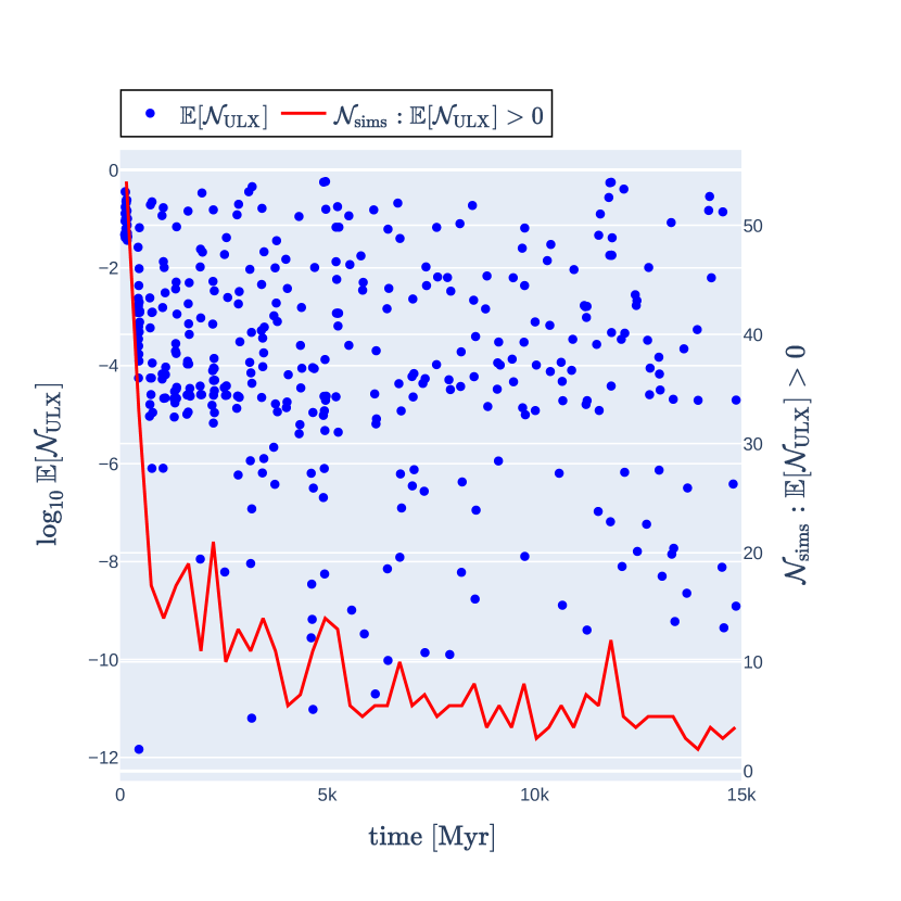
Figure 2 illustrates the temporal evolution of the expected number of ULXs333Defined as the number of ULXs weighted by their observational probability in specific evolutionary time ranges. For example, an expected value of implies that, on average, one active ULX is observed across simulations. Conversely, an expected value of indicates that, on average, ULXs are observed in a single simulation. This metric provides a probabilistic interpretation of ULX occurrence across simulations, accounting for their likelihood within evolutionary contexts. () across all simulations, accompanied by the count of simulations yielding non-zero for each time bin. The highest is observed in the initial evolutionary stages, typically within the first (first bin in Figure 2). This trend persists across all simulations, irrespective of parameter variations. These findings align with previous studies on field populations, where dynamical interactions are negligible, which reported that the ULX phase predominantly occurs in the early evolutionary stages of binaries (e.g., Wiktorowicz et al. 2017). Observational evidence also supports this conclusion (e.g. Wolter et al. 2018).
This result suggests either:
-
•
Early ULX evolution is largely independent of cluster dynamics parameters, or
-
•
Insufficient time has elapsed for dynamics to significantly influence ULX formation.
The number of simulations with decreases over time, resembling predictions for populations formed in burst-like star formation episodes (e.g. Wiktorowicz et al. 2017). In GCs, this trend may result from a combination of system age effects on ULX formation (as observed in field populations) and the interplay of positive and negative effects related to dynamics. Generally, our results indicate a higher likelihood of observing ULXs in younger stellar clusters compared to older ones.
Figure 2 reveals substantial variation in between simulations, particularly in later evolutionary phases. This variability likely stems from stochastic processes (simulation independent, i.e. resulting from random number generator seed) and varying dynamical effects (simulation dependent). The high variability in later evolutionary phases in comparison to the first bin ( – ) where low variation is observed suggest that, is affected by dynamics in at least a significant way.
The variations in the otherwise monotonically decreasing number of non-zero predictions can be attributed to randomness. The peak at and even more pronounced peak at are not correlated to any significant changes in the GC structure and are not statistically significant, therefore can be treated as anomalies.
Please note that the provided values represent predictions per cluster. To derive observational expectations, one must sum these values across all observed clusters and account for observational limitations, such as magnitude limits and resolution constraints. A detailed discussion of observational predictions will be addressed in a separate study.
3.2 Temporal Evolution and Parameter Dependence of
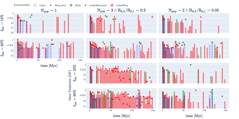
Figure 3 presents a comprehensive analysis of dependence on model parameters and its temporal evolution. The most significant effects are observed in parameters related to the environment, specifically whether the GC is tidally filling (TF) or non-tidally filling (nTF), and the general impact of dynamics (in-cluster vs. field formation). These results support the hypothesis that dynamical interactions strongly influence the formation of ULXs in dense stellar environments. In particular, the exchange process may lead to the formation of binaries that are not possible through regular formation channels. The specific trends and patterns are described below.
Non-tidally filling clusters exhibit significantly larger ULX populations compared to tidally filling clusters. This discrepancy can be attributed to the extended time frame density available for dynamical interactions to enhance progenitor formation in non-tidally filling clusters, whereas tidally filling clusters experience more early ejections. More generally, the expected number of ULXs formed in GCs is substantially higher than in corresponding field populations, particularly for non-tidally filling clusters. Typically, ULXs formed in GCs demonstrate higher rates in specific time bins, and these rates are more continuous, whereas field populations mostly exhibit isolated occurrences throughout the timeline. These relations do not apply to early evolutionary stages where all simulations show high and similar values of (see Section 3.1).
Simulations with two populations (middle column) generally produce more ULXs than those with a single population (left column). This can be attributed to the higher concentration of the second population, which enhances ULX progenitor formation. However, when the concentration is excessively high (right column), this effect is less pronounced, which supports the claim that too frequent and strong dynamical interactions can substantially destroy ULX progenitors.
The initial binary fraction appears to have a limited influence on ULX formation in GCs. For wide binaries are quickly destroyed in dynamical interactions and mostly remain binaries similar to ones for . The population of ULX progenitors remains sparse and emerges regardless of the initial relative number of binaries. Dynamical effects effectively destroy existing binaries and create new ones, a process primarily responsible for the formation of ULX progenitors at later evolutionary times. Conversely, the binary fraction influences field populations, with a positive correlation between initial binaries and ULX progenitors, as there are no external processes to destroy ULX progenitors or create new ones in isolation.
The incorporation of new features (NF) has a noticeable effect on two-population simulations with moderate concentration (; Figure 3, middle column). Simulations with NF exhibit higher values compared to those without NF (nNF). The NF do not affect field populations as they primarily relate to the time delay for the second population.
The escaper populations generally align with the ULX population formed in situ, suggesting ongoing ejection (relacation and interactions), and thus a continuous supply of ULX progenitors to the escaper population, which later become ULXs while unbound to the cluster. There are generally fewer ULXs among escapers than in in-cluster populations. However, ULXs from escapers can dominate field populations. In general, there are no significant differences in the formation time of the ULXs from escapers to those in the field. An exception occurs in simulations with relatively strong ULX formation (, ), where ULXs from escapers form at evolutionary ages not covered by field populations. For tidally filling clusters, the rate of ULX formation from escapers can exceed that of in-cluster formation, especially in simulations without new features (nNF).
3.3 Formation of ULXs
This section focuses on ULX progenitors - systems that will evolve into ULXs - and their evolution up to the initial ULX phase. It is important to note that some systems may experience multiple ULX phases interspersed with periods of quiescence or XRB phases (). Additionally, individual stars can participate in multiple ULXs, each with a different companion. This phenomenon is particularly prevalent for IMBHs (see Sect. 3.4.1).
| First Population | Second Population | |||
| binary | single | binary | single | |
| A-D(p) | ||||
| A-n | ||||
| D-A(p) | ||||
| D-n | ||||
| n-A | ||||
| n-D | ||||
| A-D(p) | ||||
| A-n | ||||
| D-A(p) | ||||
| D-n | ||||
| n-A | ||||
| n-D | ||||
| A-D(p) | ||||
| A-n | ||||
| D-A(p) | ||||
| D-n | ||||
| n-A | ||||
| n-D | ||||
Table 2 provides a comprehensive overview of ULX progenitors on ZAMS, i.e. stars that later became components of ULXs. The most common progenitors are those of pristine ULXs, i.e. binaries that do not undergo exchanges or disruptions prior to the ULX phase. In these systems, the primary typically becomes the accretor and the secondary the donor (A-D(p)). These progenitors evolve rapidly, initiating the ULX phase after approximately , in stark contrast to other progenitors which generally begin after . Pristine ULXs are observed in all simulations.
Interestingly, some pristine ULXs form where the secondary, less massive on ZAMS, becomes the accretor (D-A(p)). These progenitors are considerably rarer (about two orders of magnitude less common than A-D(p)) and typically form ULXs only in later evolutionary phases ().
Non-pristine ULXs can originate from both binary and single star progenitors on ZAMS. However, stars born in binaries more frequently become components of ULXs, even in non-pristine cases. These systems invariably undergo significant interactions, such as exchanges or disruptions, before forming a ULX. While some of these ULXs can form relatively early (), the majority emerge in later evolutionary phases (). In non-pristine ULXs, both the primary and secondary can act as either the accretor or donor with comparable probability. Our simulations did not reveal any non-pristine ULXs where both the primary and secondary are parts of ULXs (i.e., ”A-D” or ”D-A” type), though this is likely due to limited statistics rather than a physical constraint.
3.4 ULX properties
In this section we discuss the properties of in-cluster ULXs, i.e. these which reside inside the cluster. For discussion of ULXs among escapers see Section 3.7.
| group | |||||||||
|---|---|---|---|---|---|---|---|---|---|
| BH | MS | ||||||||
| BH | HG | ||||||||
| BH | CHeB | ||||||||
| BH | * | ||||||||
| NS | ** | ||||||||
| other | NS or BH | *** |
The majority of ULXs in our sample are powered by BHs accreting from various companion types. BH accretors paired with MS donors () show median masses of , while those with HG and CHeB companions ( and , respectively) have slightly lower median masses ( and , respectively). The maximum X-ray luminosities for these systems (median – ) are well above the ULX defining limit of .
NS accretors in ULXs () have median masses around . These systems typically have lower X-ray luminosities () compared to their BH counterparts, but still clearly exceed the Eddington limit for a typical NS.
The orbital characteristics of ULXs vary significantly across different groups. systems have median separations of , while systems show much tighter orbits (median ). Most ULXs in our sample have low eccentricities, suggesting that tidal forces or a common envelope phase have circularized their orbits before the onset of the ULX phase.
Duty cycles vary widely among ULX groups, with systems showing the highest median value (), while other groups have much lower values. This variability in duty cycles may explain the transient nature observed in many ULXs and has implications for their detectability (cf. Wiktorowicz et al. 2017).
A notable subset of our sample consists of IMBH-powered systems (). These ULXs are characterized by extremely high accretor masses (median ) and the highest X-ray luminosities in our sample (). Such luminous systems, called extreme-ULXs (Wiktorowicz et al. 2019), are one of the main observational candidates for IMBHs and can provide insights into their formation and properties.
The diversity in donor types across ULX groups highlights the various evolutionary pathways that can lead to ULX formation. MS, HG, and RG donors are all well-represented, suggesting that ULXs can form and persist across a wide range of stellar evolutionary stages
| label | other | |||||
|---|---|---|---|---|---|---|
| npop1-fb10-TF | ||||||
| npop1-fb10-nTF | ||||||
| npop1-fb10-nTF-nodyn | ||||||
| npop1-fb95-TF | ||||||
| npop1-fb95-nTF | ||||||
| npop1-fb95-nTF-nodyn | ||||||
| npop2-cpop05-fb10-TF | ||||||
| npop2-cpop05-fb10-nTF | ||||||
| npop2-cpop05-fb10-nTF-nodyn | ||||||
| npop2-cpop05-fb10-TF-NF | ||||||
| npop2-cpop05-fb10-nTF-NF | ||||||
| npop2-cpop05-fb10-nTF-nodyn-NF | ||||||
| npop2-cpop05-fb95-TF | ||||||
| npop2-cpop05-fb95-nTF | ||||||
| npop2-cpop05-fb95-nTF-nodyn | ||||||
| npop2-cpop05-fb95-TF-NF | ||||||
| npop2-cpop05-fb95-nTF-NF | ||||||
| npop2-cpop05-fb95-nTF-nodyn-NF | ||||||
| npop2-cpop2-fb10-TF | ||||||
| npop2-cpop2-fb10-nTF | ||||||
| npop2-cpop2-fb10-nTF-nodyn | ||||||
| npop2-cpop2-fb10-TF-NF | ||||||
| npop2-cpop2-fb10-nTF-NF | ||||||
| npop2-cpop2-fb10-nTF-nodyn-NF | ||||||
| npop2-cpop2-fb95-TF | ||||||
| npop2-cpop2-fb95-nTF | ||||||
| npop2-cpop2-fb95-nTF-nodyn | ||||||
| npop2-cpop2-fb95-TF-NF | ||||||
| npop2-cpop2-fb95-nTF-NF | ||||||
| npop2-cpop2-fb95-nTF-nodyn-NF |
Huge majority are ULXs with BH accretors (typically ) formed early in cluster evolution.
Table 4 shows a modest anticorrelation between the relative size of the and BH ULXs (Kendall777Kendall’s is preferable to Pearson’s when working with small samples and non-normal distributions, while still providing a similarly interpretable measure of association between and .’s , for , , and , respectively). The presence of IMBH results in a continuous formation of IMBH powered ULX though the cluster history which, being an independent sourse to other BH ULX groups present mostly in the early cluster evolution phases, lowers their fractional imput to the ULX population. IMBH quickly removes BHs and possibly NSs from the system (e.g. Hong et al. 2020).
3.4.1 IMBH ULXs
In this study, we define intermediate-mass black holes (IMBHs) as those with masses exceeding . IMBH ULXs were observed in 6 simulations, all featuring multiple stellar populations (npop2) and non-tidally filling initial conditions (nTF). When present, IMBHs contribute significantly to the ULX population, accounting for 16-44% of ULXs over a Hubble time (Table 4).
IMBHs form rapidly, within several Myr after the zero-age main sequence (ZAMS), classifying them as ”fast IMBHs” (Giersz et al. 2015). In simulations with delayed second populations, IMBH formation occurs 100+ Myr after the initial population. Notably, IMBH ULXs form exclusively in non-tidally filling (nTF) simulations, strenghtening the preference for denser stellar environments.
Fisher’s exact tests revealed no significant correlations between simulation parameters and IMBH formation at the 90% confidence level. However, when considering only simulations with multiple populations (pop=2) and active dynamics, a statistically significant relationship (95% confidence) emerged between the filling parameter and IMBH ULX presence, favoring non-tidally filling clusters.
| label | duty-cycle [%] | companions | ||
|---|---|---|---|---|
| npop2-cpop05-fb10-nTF | MS: 22, HeWD: 4, COWD: 3, TPAGB: 2, CHeB: 2 | |||
| npop2-cpop05-fb10-nTF-NF | MS: 41, COWD: 5, RG: 3, HeWD: 2, CHeB: 1, | |||
| EAGB: 1, TPAGB: 1, ONeWD: 1 | ||||
| npop2-cpop05-fb95-nTF | MS: 29, COWD: 13, HG: 1, HeWD: 1, RG: 1 | |||
| npop2-cpop05-fb95-nTF-NF | MS: 89, COWD: 12, TPAGB: 2, HeWD: 2, CHeB: 2, | |||
| HeGB: 1, ONeWD: 1, HG: 1 | ||||
| npop2-cpop2-fb10-nTF | MS: 32, COWD: 5, HeWD: 2, RG: 1, TPAGB: 1, | |||
| ONeWD: 1 | ||||
| npop2-cpop2-fb95-nTF | MS: 43, COWD: 11, HG: 3, HeWD: 3, TPAGB: 2, | |||
| RG: 2 |
Table 5 presents key properties of the six IMBHs observed in our simulations. IMBH ULXs typically exhibit intermittent ULX phases (duty-cycle between – with various donors, interspersed with periods of non-ULX mass accretion or mergers. Donors are mostly MS stars, the forerunner being WDs.
IMBH ULXs formed exclusively in simulations with two stellar populations and non-tidally filling initial conditions. The centrally concentrated second population facilitates stellar interactions and mergers, while nTF clusters retain more stars, particularly black holes, in central regions, extending the IMBH formation window.
3.5 ULX progenitors
The initial properties of binary systems that evolve into ULXs provide crucial insights into their formation channels and evolutionary pathways. Our results indicate that the primary distinguishing factor between ULX progenitors and the general stellar population is their higher initial mass. No other significant constraints on ZAMS properties were identified for ULX progenitors.
| group | * | mode | ||||||||
|---|---|---|---|---|---|---|---|---|---|---|
| A | A-D(p) (85%) | |||||||||
| D | A-D(p) (83%) | |||||||||
| A | A-D(p) (95%) | |||||||||
| D | A-D(p) (94%) | |||||||||
| A | A-D(p) (88%) | |||||||||
| D | A-D(p) (88%) | |||||||||
| A | A-n (100%) | |||||||||
| D | D-n (61%) | |||||||||
| A | A-D(p) (49%) | |||||||||
| D | A-D(p) (48%) | |||||||||
| other | A | A-D(p) (57%) | ||||||||
| D | A-D(p) (52%) |
Table 6 summarizes the ZAMS properties of ULX progenitors, categorized by ULX group and component role (accretor or donor). Accretor progenitors typically have higher ZAMS masses () than their companions (), consistent with being predominantly formed from primary stars ().
The majority of ULX progenitors originate in binary systems (), with most maintaining their original pairing to form the ULX (, except for the group). For accretors in the and groups, , indicating no preference between single and binary star origins.
Initial separations () exhibit a highly skewed distribution, with group progenitors typically having much wider separations than other groups. Values for the group are not particularly informative as these stars do not become components of ULXs without undergoing strong dynamical interactions. All groups show a preference for lower initial eccentricities ().
The group shows distinct characteristics compared to other groups. It has the lowest ZAMS masses for both accretors and donors, a unique dominant formation modes (A-n for accretors and D-n for donors), and the lowest . The and groups exhibit similar patterns, with high ZAMS masses and a strong preference for the A-D(p) formation mode. The group has the highest fraction of ULXs formed from escapers ().
3.6 ULX descendants
| D | E | X | M | O | |
|---|---|---|---|---|---|
| npop1-fb10-TF | |||||
| npop1-fb10-nTF | |||||
| npop1-fb95-TF | |||||
| npop1-fb95-nTF | |||||
| npop2-cpop05-fb10-TF | |||||
| npop2-cpop05-fb10-TF-NF | |||||
| npop2-cpop05-fb10-nTF | |||||
| npop2-cpop05-fb10-nTF-NF | |||||
| npop2-cpop05-fb95-TF | |||||
| npop2-cpop05-fb95-TF-NF | |||||
| npop2-cpop05-fb95-nTF | |||||
| npop2-cpop05-fb95-nTF-NF | |||||
| npop2-cpop2-fb10-TF | |||||
| npop2-cpop2-fb10-TF-NF | |||||
| npop2-cpop2-fb10-nTF | |||||
| npop2-cpop2-fb10-nTF-NF | |||||
| npop2-cpop2-fb95-TF | |||||
| npop2-cpop2-fb95-TF-NF | |||||
| npop2-cpop2-fb95-nTF | |||||
| npop2-cpop2-fb95-nTF-NF |
The fate of ULX systems after their active phase provides valuable insights into their evolutionary pathways and potential contributions to other astrophysical phenomena. Table 7 summarizes the various outcomes for ULX systems across different simulation configurations.
ULX systems can undergo several fates: disruption, escape from the cluster, exchange interactions, mergers, or other outcomes. The distribution of these fates appears largely stochastic across different simulation parameters. Systems categorized as ”other” typically experience no significant events for the remainder of their evolution and are predominantly NS/BH + WD or DCOs at the end of simulation.
Merger events typically occur after the ULX phase. Double compact objects (DCOs) form in of cases, with of them being ejected from the cluster before merger or the end of simulation. These DCOs that remain in the cluster may contribute to the population of gravitational wave (GW) sources with merger rate of .
Disruptions may result from dynamical interactions or binary evolution. In exchanges, at least one of the components continues evolution as part of some other binary. Our results suggest, that in initially more centrally concentrated environment (nTF) there are more disruptions and exchanges after the ULX phases, then in other simulations.
3.7 ULXs among escapers
Cluster-formed binaries are frequently ejected, suggesting that some field ULXs may originate from GCs. These ULX progenitors become unbound from their parent clusters and initiate the ULX phase while residing in the galactic field, evolving as isolated binaries.
Figure 3 illustrates the expected numbers and ages of ULXs among escapers. Generally, escaper ULXs coexist in similar numbers and at comparable evolutionary times as their in-cluster counterparts, except the very early phase of cluster evolution (). Table 8 presents a detailed comparison of properties between in-cluster and escaper ULXs.
| escaper | in-cluster | |||
|---|---|---|---|---|
| NS | BH | NS | BH | |
| count | ||||
| Typ. companion | HeMS (70%) | CHeB (80%) | HG (74%) | HG (55%) |
Escaper ULXs exhibit several distinct characteristics compared to their in-cluster counterparts. They tend to have lower-mass accretors and donors, with median masses of and , respectively, compared to and for in-cluster ULXs. Escaper ULXs also have tighter orbits (median vs. ) and a significantly higher fraction of neutron star accretors ( vs. ). The median maximum X-ray luminosity of escaper ULXs () is slightly lower than that of in-cluster ULXs ().
Notably, escaper ULXs are less numerous, with a median count of compared to for in-cluster ULXs. They also typically have more evolved companion stars, with having CHeB donors compared to HG donors for in-cluster ULXs. The duty cycles and ULX phase onset times are similar for both populations.
The ejection processes preferentially remove less massive systems, explaining the lower masses observed in escaper ULXs. The higher fraction of neutron star accretors among escapers could be due to the higher natal kicks and retention of more massive black holes within the cluster potential.
These findings have important implications for understanding the origin and evolution of field ULXs. A significant fraction of observed field ULXs may have originated in globular clusters, which could explain some of the observed diversity in ULX populations. Furthermore, the differences between escaper and in-cluster ULXs provide valuable insights into how environment and dynamical history can influence the properties of these extreme systems.
In conclusion, our simulations reveal that escaper ULXs form a significant and distinct population with properties that differ from their in-cluster counterparts. These differences provide valuable insights into the formation and evolution of ULXs in various environments and highlight the need for comprehensive observational surveys to fully characterize the ULX population across different galactic settings.
4 Discussion
The results presented in this study are specific to the simulations employed and may not capture general trends applicable to all GC environments. The parameter choices were carefully tailored to conditions characteristic of GCs, informed by insights from analogous studies.
A key limitation in the broader study of ULXs in GCs is the paucity of confirmed observations within the Milky Way and its immediate vicinity. The substantial distances involved often complicate the detection and characterization of low-luminosity donor stars, which are believed to comprise a significant fraction of ULX donors (e.g. Wiktorowicz et al. 2017).
Furthermore, a critical challenge for this study lies in the difficulty of unambiguously differentiating GC-associated ULXs from those in the field environment. Observational uncertainties frequently obscure the distinction, as localization on the plane of a GC does not inherently confirm membership within the cluster. Determining the precise distance to the source is often fraught with uncertainties, leaving room for the possibility that the ULX is a foreground or background source, merely coincident with the GC in projection. This ambiguity highlights the importance of complementary approaches, such as proper motion studies or radial velocity measurements, to confirm GC membership conclusively.
4.1 Comparison with field populations
We find a high fraction of NS accretors among escapers () compared to in-cluster ULXs (). This is similar to the predictions of Wiktorowicz et al. (2019), who found that NS ULXs outnumber BH ULXs in regions with constant star formation and solar metallicity for ages above .
The properties of our escaper NS ULXs show some similarities with typical field NS ULXs described by Wiktorowicz et al. (2017). They found that field NS ULXs typically have NS accretors and Red Giant donors. This is comparable to our escaper ULXs with NS accretors, which have low-mass evolved (HeMS) donors. Our systems are very compact () which may explain the lower fraction of giant donors.
Our escaper NS ULXs have a median maximum X-ray luminosity of , with a few BH ULXs exceeding . This stays in contrast to the field populations, where a significant fraction of more luminous sources is also expected (e.g., Wiktorowicz et al. 2015). In the case of globular clusters, we find that such extreme ULXs are more likely to be retained within the cluster.
The formation pathways of escaper ULXs may differ from those in the field. For instance, Fragos et al. (2015) studied the formation of NS ULXs like M82 X-2, finding that systems with – donor stars could produce such ULXs. In contrast, our escaper NS ULXs have lower donor masses (), suggesting a different formation pathway.
The temporal distribution of ULXs in our simulations differs from that observed in field populations. Kuranov et al. (2021) found that the maximum number of ULXs ( for a star formation rate of ) is reached after the beginning of star formation in field populations. Our escaper ULXs show a different temporal distribution with a more uniform appearance of escaper ULXs through the GC lifespan.
It is worth noting that even field populations are not entirely free from dynamical influences. Klencki et al. (2017) showed that wide binaries in the field are affected by multiple weak interactions (fly-bys) which can impact binary evolution. This suggests that the distinction between cluster-formed and field-formed ULXs may not be as clear-cut as previously thought, and that dynamical effects could play a role in shaping ULX populations across various environments.
4.2 Counterparts
The identification and characterization of ULX counterparts is crucial for understanding the nature of these systems, yet it remains a significant observational challenge (Heida et al. 2016; Wiktorowicz et al. 2021). While many ULXs are found in star-forming regions, their faintness in the optical and near-infrared (NIR), combined with the crowded environments, makes it difficult to confirm donor stars (López et al. 2020; Allak et al. 2022; Heida et al. 2019). The observed optical emission can be a combination of light from the accretion disc and/or the donor star (Heida et al. 2016). Accurate astrometry is essential for identifying counterparts, particularly for distinguishing between potential candidates within the error radii of ULX positions (Allak et al. 2022).
Red supergiants (RSGs) have also been identified as potential donors in ULXs (Heida et al. 2016, 2019; López et al. 2020). However, several sources initially classified as RSGs have been found to be nebulae, making the classification challenging (López et al. 2020). Actually, the fraction of ULXs with RSG donors is potentially higher than predicted by binary evolution models (López et al. 2020).
It’s important to note that observational biases exist that favour the detection of more luminous and massive companions, such as RSGs (e.g. Heida et al. 2019). Additionally, systems may be old, which makes it less likely for the donor to be a supergiant (Wiktorowicz et al. 2017). Therefore, ULX counterparts remain ’candidates’ and need more thorough survey searches (Wiktorowicz et al. 2021).
4.3 Expectations for Antennae galaxy
The correlation between X-ray source positions and stellar clusters has been previously noted in starburst galaxies (e.g. Kaaret et al. 2004). The study of the Antennae galaxies by Poutanen et al. (2013) reveals a highly significant association between bright X-ray sources and stellar clusters, although most of these X-ray sources are located outside of the clusters.
This finding is consistent with the idea that many ULXs are massive X-ray binaries that have been ejected from their birth clusters, rather than being intermediate mass black holes (IMBHs). Both ULXs and XRBs show a strong association with young stellar clusters, indicating a common origin.
The displacements of ULXs from centres of their neighbouring star clusters are statistically significant and range up to 300 parsecs. This is likely due to the ejection of massive binaries from the clusters.
The ejection mechanism suggested by Poutanen et al. (2013), supernova kicks and few-body encounters are consistent with the results of our work, where ULX among escapers have much higher NS accretor fraction and much smaller separations.
Poutanen et al. (2013) provides evidences that dynamical ejection can be a major formation mechanism for these systems in the field.
4.4 Future prospects
Future studies of ULXs in globular clusters should include more simulations to better estimate statistical effects, errors, and the significance of conclusions. A more consistent survey of the parameter space is needed, as well as the incorporation of evolutionary parameters (both stellar and binary evolution) beyond dynamical ones.
In the future work we plan to include the effect of beaming in ULXs (e.g. Lasota & King 2023). Beaming increases the apparent luminosity of ULXs, but decreases the probability of observation due to possible misalignment (Wiktorowicz et al. 2019; Khan et al. 2022). Population synthesis simulations, Wiktorowicz et al. (e.g. 2019) indicate that the majority of neutron star (NS) ULXs are beamed. The beaming factor is dependent on the mass transfer rate, with higher mass transfer rates resulting in stronger beaming (King 2009).
Additionally, the importance of wind Roche-lobe overflow (WRLOF; see e.g., Wiktorowicz et al. 2021; Zuo et al. 2021, and references therein) for NS ULXs with (super)giant donors should be explored. WRLOF can lead to stable mass transfer even with large mass ratios, and can boost mass transfer rates to reach ULX luminosity levels.
5 Conclusions
This study presents the first numerical investigation into the formation and evolution of ULXs within GCs, utilizing a subset of simulations to explore parameter dependencies.
Our simulations reveal that dynamical interactions may play a critical role in ULX formation, particularly in environments with high stellar density. Even if the initial binary fraction is low, the interactions can produce many ULXs. On average, we find that approximately of ULXs in our simulations have BH companions and the number can be even higher for very young clusters (). Among escaper, ULXs have a much higher fraction of NS accretors ().
Our simulations show that the ratio of escaper ULXs to in-cluster ULXs is approximately 1:7, but nearly 2:1 for ULX with NS accretors. This ratio is the highest in tidally filling clusters, even with high initial binary fractions, where rapid ejections can hinder in-cluster ULX formation by ejecting the progenitors.
Our findings suggest that the relative scarcity of ULXs observed in GCs may be attributed to the advanced age of their stellar populations. In contrast, field populations usually have continuous star formation.
The apparent absence of ULXs in Milky Way GCs aligns more closely with our models of initially tidally filling clusters rather than non-tidally filling ones.
Furthermore, our results suggest that field populations may be significantly ”polluted” by ULXs ejected from GCs (escapers), which could contribute to the relative underrepresentation of ULXs in GCs compared to field environments. Escapers can have properties very similar to the field populations or form dinsinct configurations.
Future observational efforts should prioritize the comparison of ULX properties across diverse environments, including GCs and the galactic field. Such studies will be critical for validating our theoretical predictions and advancing our understanding of the diverse formation channels of ULXs.
Acknowledgments
GW, MG, AH, LH were supported by the Polish National Science Center (NCN) through the grant 2021/41/B/ST9/01191 AA acknowledges support for this paper from project No. 2021/43/P/ST9/03167 co-funded by the Polish National Science Center (NCN) and the European Union Framework Programme for Research and Innovation Horizon 2020 under the Marie Skłodowska-Curie grant agreement No. 945339. For the purpose of Open Access, the authors have applied for a CC-BY public copyright license to any Author Accepted Manuscript (AAM) version arising from this submission.
Data Availability
Data available on request.
References
- Allak et al. (2022) Allak, S., Akyuz, A., Sonbas, E., & Dhuga, K. S. 2022, MNRAS, 515, 3632
- Bachetti et al. (2014) Bachetti, M., Harrison, F. A., Walton, D. J., et al. 2014, Nature, 514, 202
- Bastian & Lardo (2018) Bastian, N. & Lardo, C. 2018, ARA&A, 56, 83
- Belczynski et al. (2008) Belczynski, K., Kalogera, V., Rasio, F. A., et al. 2008, ApJS, 174, 223
- Belloni et al. (2017) Belloni, D., Zorotovic, M., Schreiber, M. R., et al. 2017, MNRAS, 468, 2429
- Casertano & Hut (1985) Casertano, S. & Hut, P. 1985, ApJ, 298, 80
- Dage et al. (2021) Dage, K. C., Kundu, A., Thygesen, E., et al. 2021, MNRAS, 504, 1545
- Dage et al. (2020) Dage, K. C., Zepf, S. E., Thygesen, E., et al. 2020, MNRAS, 497, 596
- Fragos et al. (2015) Fragos, T., Linden, T., Kalogera, V., & Sklias, P. 2015, ApJ, 802, L5
- Fregeau et al. (2004) Fregeau, J. M., Cheung, P., Portegies Zwart, S. F., & Rasio, F. A. 2004, MNRAS, 352, 1
- Fryer et al. (2012) Fryer, C. L., Belczynski, K., Wiktorowicz, G., et al. 2012, ApJ, 749, 91
- Giersz et al. (2024) Giersz, M., Askar, A., Hypki, A., et al. 2024, arXiv e-prints, arXiv:2411.06421
- Giersz et al. (2015) Giersz, M., Leigh, N., Hypki, A., Lützgendorf, N., & Askar, A. 2015, MNRAS, 454, 3150
- Gnedin & Ostriker (1997) Gnedin, O. Y. & Ostriker, J. P. 1997, ApJ, 474, 223
- Gratton et al. (2019) Gratton, R., Bragaglia, A., Carretta, E., et al. 2019, A&A Rev., 27, 8
- Heida et al. (2019) Heida, M., Harrison, F. A., Brightman, M., et al. 2019, ApJ, 871, 231
- Heida et al. (2016) Heida, M., Jonker, P. G., Torres, M. A. P., et al. 2016, MNRAS, 459, 771
- Hellström et al. (2024) Hellström, L., Giersz, M., Hypki, A., et al. 2024, A&A, 690, A112
- Hénon (1971) Hénon, M. 1971, Ap&SS, 13, 284
- Hobbs et al. (2005) Hobbs, G., Lorimer, D. R., Lyne, A. G., & Kramer, M. 2005, MNRAS, 360, 974
- Hong et al. (2020) Hong, J., Askar, A., Giersz, M., Hypki, A., & Yoon, S.-J. 2020, MNRAS, 498, 4287
- Hurley et al. (2000) Hurley, J. R., Pols, O. R., & Tout, C. A. 2000, MNRAS, 315, 543
- Hurley et al. (2002) Hurley, J. R., Tout, C. A., & Pols, O. R. 2002, MNRAS, 329, 897
- Hypki & Giersz (2013) Hypki, A. & Giersz, M. 2013, MNRAS, 429, 1221
- Hypki et al. (2022) Hypki, A., Giersz, M., Hong, J., et al. 2022, MNRAS, 517, 4768
- Hypki et al. (2025) Hypki, A., Vesperini, E., Giersz, M., et al. 2025, A&A, 693, A41
- Irwin et al. (2010) Irwin, J. A., Brink, T. G., Bregman, J. N., & Roberts, T. P. 2010, ApJ, 712, L1
- Irwin et al. (2016) Irwin, J. A., Maksym, W. P., Sivakoff, G. R., et al. 2016, Nature, 538, 356
- Ivanova et al. (2008) Ivanova, N., Heinke, C. O., Rasio, F. A., Belczynski, K., & Fregeau, J. M. 2008, MNRAS, 386, 553
- Ivanova et al. (2005) Ivanova, N., Rasio, F. A., Lombardi, Jr., J. C., Dooley, K. L., & Proulx, Z. F. 2005, ApJ, 621, L109
- Kaaret et al. (2004) Kaaret, P., Alonso-Herrero, A., Gallagher, J. S., et al. 2004, MNRAS, 348, L28
- Kaaret et al. (2017a) Kaaret, P., Feng, H., & Roberts, T. P. 2017a, ARA&A, 55, 303
- Kaaret et al. (2017b) Kaaret, P., Feng, H., & Roberts, T. P. 2017b, ARA&A, 55, 303
- Kamlah et al. (2022) Kamlah, A. W. H., Leveque, A., Spurzem, R., et al. 2022, MNRAS, 511, 4060
- Khan et al. (2022) Khan, N., Middleton, M. J., Wiktorowicz, G., et al. 2022, MNRAS, 509, 2493
- Kiminki & Kobulnicky (2012) Kiminki, D. C. & Kobulnicky, H. A. 2012, ApJ, 751, 4
- King (2009) King, A. R. 2009, MNRAS, 393, L41
- Klencki et al. (2017) Klencki, J., Wiktorowicz, G., Gładysz, W., & Belczynski, K. 2017, MNRAS, 469, 3088
- Kobulnicky et al. (2014) Kobulnicky, H. A., Kiminki, D. C., Lundquist, M. J., et al. 2014, ApJS, 213, 34
- Kroupa (1995) Kroupa, P. 1995, MNRAS, 277, 1491
- Kroupa (2001) Kroupa, P. 2001, MNRAS, 322, 231
- Kulkarni et al. (1993) Kulkarni, S. R., Hut, P., & McMillan, S. 1993, Nature, 364, 421
- Kuranov et al. (2021) Kuranov, A. G., Postnov, K. A., & Yungelson, L. R. 2021, Astronomy Letters, 47, 831
- Lasota & King (2023) Lasota, J.-P. & King, A. 2023, MNRAS, 526, 2506
- López et al. (2020) López, K. M., Heida, M., Jonker, P. G., et al. 2020, MNRAS, 497, 917
- Maccarone et al. (2007) Maccarone, T. J., Kundu, A., Zepf, S. E., & Rhode, K. L. 2007, Nature, 445, 183
- Maccarone et al. (2011) Maccarone, T. J., Kundu, A., Zepf, S. E., & Rhode, K. L. 2011, MNRAS, 410, 1655
- Milone & Marino (2022) Milone, A. P. & Marino, A. F. 2022, Universe, 8, 359
- Oh et al. (2015) Oh, S., Kroupa, P., & Pflamm-Altenburg, J. 2015, ApJ, 805, 92
- Piotto et al. (2015) Piotto, G., Milone, A. P., Bedin, L. R., et al. 2015, AJ, 149, 91
- Pooley et al. (2003) Pooley, D., Lewin, W. H. G., Anderson, S. F., et al. 2003, ApJ, 591, L131
- Poutanen et al. (2013) Poutanen, J., Fabrika, S., Valeev, A. F., Sholukhova, O., & Greiner, J. 2013, MNRAS, 432, 506
- Renzini et al. (2015) Renzini, A., D’Antona, F., Cassisi, S., et al. 2015, MNRAS, 454, 4197
- Roberts et al. (2012) Roberts, T. P., Fabbiano, G., Luo, B., et al. 2012, ApJ, 760, 135
- Sana et al. (2012) Sana, H., de Mink, S. E., de Koter, A., et al. 2012, Science, 337, 444
- Shakura & Sunyaev (1973) Shakura, N. I. & Sunyaev, R. A. 1973, A&A, 24, 337
- Shih et al. (2010) Shih, I. C., Kundu, A., Maccarone, T. J., Zepf, S. E., & Joseph, T. D. 2010, ApJ, 721, 323
- Sivakoff et al. (2005) Sivakoff, G. R., Sarazin, C. L., & Jordán, A. 2005, ApJ, 624, L17
- Spitzer & Hart (1971) Spitzer, Jr., L. & Hart, M. H. 1971, ApJ, 164, 399
- Stodolkiewicz (1986) Stodolkiewicz, J. S. 1986, Acta Astron., 36, 19
- Thygesen et al. (2023) Thygesen, E., Sun, Y., Huang, J., et al. 2023, MNRAS, 518, 3386
- Walton et al. (2022) Walton, D. J., Mackenzie, A. D. A., Gully, H., et al. 2022, MNRAS, 509, 1587
- Webb et al. (2013) Webb, J. J., Harris, W. E., Sills, A., & Hurley, J. R. 2013, ApJ, 764, 124
- Wiktorowicz et al. (2021) Wiktorowicz, G., Lasota, J.-P., Belczynski, K., et al. 2021, ApJ, 918, 60
- Wiktorowicz et al. (2019) Wiktorowicz, G., Lasota, J.-P., Middleton, M., & Belczynski, K. 2019, ApJ, 875, 53
- Wiktorowicz et al. (2017) Wiktorowicz, G., Sobolewska, M., Lasota, J.-P., & Belczynski, K. 2017, ApJ, 846, 17
- Wiktorowicz et al. (2015) Wiktorowicz, G., Sobolewska, M., S\kadowski, A., & Belczynski, K. 2015, ApJ, 810, 20
- Wolter et al. (2018) Wolter, A., Fruscione, A., & Mapelli, M. 2018, ApJ, 863, 43
- Zuo et al. (2021) Zuo, Z.-Y., Song, H.-T., & Xue, H.-C. 2021, A&A, 649, L2