Enumeration of Colored Tilings on Graphs via Generating Functions
Abstract.
In this paper, we study the problem of partitioning a graph into connected and colored components called blocks. Using bivariate generating functions and combinatorial techniques, we determine the expected number of blocks when the vertices of a graph , for in certain families of graphs, are colored uniformly and independently. Special emphasis is placed on graphs of the form , where is the path graph on vertices. This case serves as a generalization of the problem of enumerating the number of tilings of an grid using colored polyominoes.
Key words and phrases:
Tiling; polyomino; generating function.2010 Mathematics Subject Classification:
05A15, 05A051. Introduction
In this paper, we address the problem of enumerating the number of tilings of an grid using colored polyominoes. This problem is part of a broader class of results concerning the enumerating of ways to partition a collection of objects into smaller sets according to specific rules. One of the simplest examples in this context is counting the number of tilings of a rectangle using vertical and horizontal dominoes, which is given by the Fibonacci number , see [1] for a generalization of this problem on surfaces. The more general problem of tiling an grid was independently solved by Temperley and Fisher [11] and Kasteleyn [4]. The solution is elegantly expressed by the following formula:
| (1) |
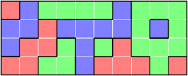
In the plane , a cell is a unit square with vertices that have integer coordinates. A polyomino is a finite set of cells whose interior is connected. A variation of the previous problem is to consider the number of tilings of an grid using polyominoes colored with one of colors, with the condition that two adjacent polyominoes, that is, those sharing at least one edge, must have different colors. A tiling of this type is called a -colored tiling. For example, Figure 1 shows a 3-colored tiling of a grid. Note that this example consists of 11 polyominoes.
Richey [8] shows that exists and is finite, where is the expected number of polyominoes on an grid. Mansour [5] uses automata theory to obtain a solution for grids with height at most 3. Rolin and Ugolnikova [9] also apply automata theory to the case of square polyominoes of sizes and . Ramírez and Villamizar [6] consider this problem for square and hexagonal grids by using generating functions. Recently, Došlic and Podrug [3] also explored the case of hexagonal grids. Bodini [2] addressed a related problem, known as rectangular shape partitions.
This combinatorial problem can be described in terms of graphs [7]. Let and be two undirected graphs. The product of and is defined as , where
Let be a path graph, which is a simple graph with vertices arranged in a linear sequence such that two vertices are adjacent if they are consecutive in the sequence, and non-adjacent otherwise. A grid graph of size is defined as the product .
Let be an undirected graph. Two non-empty disjoint subsets are said to be neighbors if there exists an edge such that and . A -colored partition of the vertices of is a partition , with , such that each induces a connected subgraph of , all vertices in are colored with one of colors, and any pair of neighboring sets and are colored with different colors. Each set is called a block of the partition, and the number of blocks is called the size of the partition. For example, Figure 2 shows a 3-colored partition of size of .
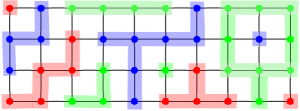
The problem of counting -colored tilings of the grid is equivalent to counting -colored partitions of the graph . For example, the partition shown in Figure 2 corresponds to the 3-colored tiling given in Figure 1.
Given a -colored partition , we use to denote the size of the partition . Let be an undirected graph and denote by the set of all -colored partitions of . The random variable gives the size of a random -colored partition in .
2. Colored Partitions on Trees
The aim of this section is to enumerate the number of -colored partitions of a given tree. Recall that a tree is a connected graph with no cycles. A perfect binary tree is a tree in which every vertex has either or children, and all leaves are at the same height. Let denote the set of perfect binary trees in which the height of each leaf is .
For fixed positive integers and , we define the bivariate generating function
Let denote the coefficient of in the generating function , that is, .
Lemma 2.1.
For all , we have
Proof.
We begin by noting that for , we have , since there is only one vertex in the tree. For , a perfect binary tree of height consists of a root connected to two perfect binary trees of height . Using this structure, we obtain the following recurrence relation:
Let . Then, we can write
Therefore, we have
Simplifying this expression, we obtain the desired result. ∎
For example, when and , the polynomial is
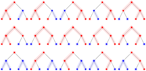
In Figure 3, we illustrate the corresponding 2-colored partitions of size 3 for the perfect binary tree , where the root is colored red.
From the previous lemma, we can see that
Using Lemma 2.1, if we differentiate and normalize by , the following corollary follows.
Corollary 2.2.
The expected number of blocks when uniformly and independently coloring a perfect binary tree with levels using colors is given by
We can generalize this result to trees with vertices. Let be a tree with vertices. We introduce the bivariate generating function
Theorem 2.3.
For all , we have
Proof.
To prove this result, consider an arbitrary vertex of the tree, which we designate as the root, and color it with one of the available colors. This contributes the term to the generating function. Next, for each child of the root, there are two possibilities: either we color the child the same as the root, which does not create a new block, or we color the child differently. If we choose a different color, we must select one from the remaining colors, thus creating a new colored block. These options translate into the term . Repeating this process for each subsequent level down to the leaves of the tree results in the final expression. ∎
Corollary 2.4.
The expected number of blocks when uniformly and independently coloring a tree with vertices using colors is given by
Proof.
Taking the derivative of the generating function with respect to , we obtain
Evaluating this expression at , we have
Simplifying the expression, we obtain the desired result. ∎
As an example, consider the case of the grid , which is a tree (the path graph with vertices). In this case, we recover Theorem 1 in [6].
3. Colored Partitions on the Cycle Graph
A walk in a graph is a sequence of vertices , not necessarily distinct, such that each pair of consecutive vertices is an edge in the graph. The length of a walk corresponds to the number of edges, which is equivalent to the integer . A closed walk is a walk in which the first vertex is the same as the last vertex .
Let denote the cycle graph on the vertices. We introduce the bivariate generating function
where is the number of -colored partitions of the cycle graph of size .
Theorem 3.1.
The number of -colored partitions of size for the cyclic graph , for , is given by
Moreover, its bivariate generating function is given by
Proof.
If the size of the partition is one, then all vertices are colored the same color. Consequently, we can choose this color in ways. For , consider the choice of colors as walks in a complete graph with vertices, where each vertex is labeled with one of the colors. The walk starts and ends at either the same color (which means that the size of the partition decreases by one) or at different colors. Recall the known formula (cf. [10, p. 5]) for the number of closed walks of size in the complete graph , given by
and the number of walks that start and end at different vertices is given by
The number of ways to select the blocks is given by the number of integer compositions of into parts, which is . Depending on the colors we choose, there will either be blocks or blocks. If the walk starts and ends in different colors, then we have blocks. If the walk starts and ends at the same color, then we obtain blocks. Thus, by considering both cases for the starting and ending colors, the number of -colored partitions of size is given by
The last equality is Pascal’s recursion for the binomial coefficients. Finally, using the expression for the number of -colored partitions, we obtain the bivariate generating function
| (2) | ||||
| (3) |
The result follows by completing the geometric series. ∎
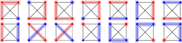
For example, when , and , we have . In Figure 4, we illustrate the corresponding 2-colored partitions of size 4 for the cycle graph , where two consecutive vertices are colored red.
Corollary 3.2.
The expected number of blocks when uniformly and independently coloring a cycle graph with vertices using colors is given by
Proof.
Starting with the expression of the generating function in (2), we differentiate with respect to to obtain
Evaluating this derivative at gives the desired result. ∎
4. Colored Partitions on the Complete Graph
Let denote the complete graph on vertices. We introduce the exponential bivariate generating function
where denotes the number of -colored partitions of size on the complete graph .
Theorem 4.1.
The number of -colored partitions of size for the complete graph , for , is given by
Moreover, its exponential bivariate generating function is given by
Proof.
To construct a -colored partition of size , we first choose colors from the available colors, which can be done in ways. Next, we partition the vertices of the complete graph into disjoint non-empty blocks and assign one of chosen colors to each block. This can be done in ways, where are the Stirling numbers of the second kind. The assignment of the colors gives the -colored partitions because the graph is complete.
Using the above, we have that the generating function is given by
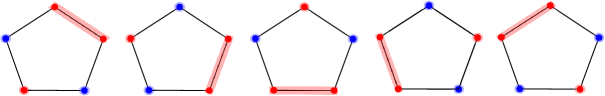
For example, when , and , we have . In Figure 5, we illustrate the corresponding 2-colored partitions of size 2 for the complete graph .
Corollary 4.2.
The expected number of blocks when uniformly and independently coloring a complete graph with vertices using colors is given by
Proof.
Using Theorem 4.1, to compute the expected value, we need to find the coefficient of in the expansion of
Evaluating at , we have . Extracting the coefficient of from the expansion, we obtain
Dividing by the total number of colorings, , we have the expected value
5. Colored Partitions on the Complete Bipartite Graph
Let denote the complete bipartite graph on and vertices.
Theorem 5.1.
The expected number of blocks when uniformly and independently coloring a complete bipartite graph using colors is given by
Proof.
A colored partition is formed by assigning a color to each vertex of a bipartite graph. If the same color is used on the vertices of both parts, they will merge into a single block. Therefore, the number of blocks is equal to the total number of vertices minus the number of vertices that share the same color in both parts. This implies that the expected number of blocks is
| (4) |
We will divide the sum into two parts:
-
(1)
First, consider
This summation is equivalent to iterating over each element on , one block of the graph, and counting the pairs of functions where is in the image of . By symmetry, we find that this summation is equal to
To compute the size of this set, we iterate over the size of the image of and use the fact that a function is surjective over its image. Given the size of the image, we choose an element of the image, leading to the result
Using the computation from the proof of Corollary 4.2, we obtain that this summation is equal to
-
(2)
Next, consider
This summation is equivalent to iterating over the colors and counting the number of function pairs that include that color in their image. By symmetry, we find that the summation is equal to
Substituting these results into the expression in (4) gives the result. ∎
6. Colored Partitions in the Cartesian Product
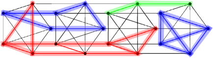
In this section, we enumerate the -colored partitions for the graph product for . For example, Figure 6 shows a 3-colored partition of size for the graph .
6.1. The case .
In this section, we provide the explicit bivariate generating function for the -colored partitions of for all . For fixed positive integers and , we define the bivariate generating function as
where denotes the set of -colored partitions of , and is the size of the partition .
Theorem 6.1.
The bivariate generating function is given by , where
and
Moreover, .
Proof.
Let denote the set of -colored tilings in such that the last triangle is colored with exactly different colors, where . For a -colored partition , we denote the last triangle of by .
Define the bivariate generating functions
It is clear that .
Let be a -colored partition in . If , then , and its contribution to the generating function is the term , as it must be monochromatic. If , then can be decomposed as , where is monochromatic, and , for . The decomposition leads to:
-
•
Case 1 (). In this case, and may or may not share the same color. Therefore, the generating function is given by
-
•
Case 2 (). Here there are two possibilities, and either coincide in one of the colors of or are colored differently. Thus, the generating function is
-
•
Case 3 (). Similarly, and may coincide in one of the colors of or be entirely different. The generating function for this case is
Table 1 illustrates the three cases discussed above.
| Case 1 |
| Case 2 |
| Case 3 |
Combining these, we obtain the following functional equation:
For , we analyze its decomposition as shown in Table 2. Each case yields terms based on the interaction of with .
| Case 1 |
| Case 2 |
![[Uncaptioned image]](/html/2501.06008/assets/x11.png) |
| Case 3 |
![[Uncaptioned image]](/html/2501.06008/assets/x12.png) |
From this decomposition the generating function for satisfies:
Finally, let be a -colored partition in . Again, from a similar argument as before, we can obtain the different possible decompositions, as show in Table 3.
| Case 1 |
| Case 2 |
![[Uncaptioned image]](/html/2501.06008/assets/x14.png) |
| Case 3 |
![[Uncaptioned image]](/html/2501.06008/assets/x15.png) |
From this decomposition we obtain the functional equation:
Since , we obtain a system of four linear equations with four unknowns , and . Solving the system for yields the desired result. ∎
Corollary 6.2.
The expected number of blocks when uniformly and independently coloring the graph with vertices using colors is given by
6.2. The general case
In this section, we present a general approach for counting the number of -colored partitions of the graph . Let denote the set of possible -colored partitions for For fixed positive integers and , we introduce the following bivariate generating function:
| (5) |
To determine the generating function , we establish a system of equations indexed by the possible -colored partitions of the complete graph .
Definition 6.3.
Let denote the set of sequences of subsets of that are pairwise disjoint and whose union is . Formally,
First, notice that these sequences can correspond to any configuration in and they are in bijection with functions from to by considering the preimages. For a given , we denote by the number of indices for which , these are the colors that we have used at least once on a vertex of the corresponding configuration. For fixed integers and , and a given , consider the following bivariate function:
where are the -colored partitions of that end in the configuration specified by . In this way, we would have
We have now the following system of equations:
Consider, further, the following equivalence relation over the set , defined by if and only if there exists a permutation , where denotes the group of permutations on elements, such that for all .
Notice that , since these are all possible colorings for the complete graph. However, the number of distinct equivalence classes in is given by the coefficient of in the Gaussian binomial coefficient . This is because the coefficient of in counts the number of partitions of into or fewer parts, where each part is bounded above by .
The size of each equivalence class is given by
The first multinomial considers the choice of each set based on cardinality, while the second multinomial considers a permutation on the sequence of cardinals. Here, denotes the number of sets in the sequence that have size .
Example 6.4.
Consider and , then there are possible colorings listed below as elements in
The quotient is given by , where the tuple represents the element in . The sizes of the classes are given by
This equivalence relation enables us to reduce the number of variables in the system of equations used to compute . This reduction is possible due to the following proposition, which stems from the fact that the equivalence relation captures both the symmetries of the complete graph and the symmetries of the color permutations.
Proposition 6.5.
If , then .
Using the proposition above, and for , we can express the generating functions in terms of the tuples , such that for any . As an example of this reduction, we compute the generating function for the number of -colored partitions of the graph .
Theorem 6.6.
The bivariate generating function is given by
Proof.
Using the description above and Example 6.4, we consider three distinct variables , , and . Each variable corresponds to a different configuration for the last copy of , and each contributes differently to the bivariate generating function. The contribution of each variable is determined by the size of the corresponding equivalence class. Therefore, we have
| (6) |
The following relations arise when considering each possible pair of contiguous copies of :
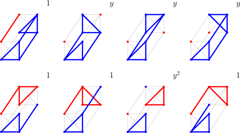
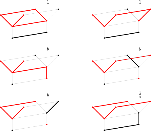
As an example, consider . Figure 7 illustrates all eight possible combinations that can result in a configuration ending with after a previous configuration that also ends in . By solving this system of equations and substituting the solution into (6), the theorem follows.
∎
Corollary 6.7.
The expected number of blocks when uniformly and independently coloring the graph with vertices using two colors is given by
Using this approach, we wrote a Python code111 https://github.com/Phicar/ColoredColumns/blob/main/CompleteGraphGenFunc.py to calculate the generating functions. For example, this method produces the following generating functions:
The results above lead to the following expression for the expected number of blocks in a random -colored partition of the graph .
Theorem 6.8.
The expected size of a -colored partition on the graph assuming each vertex is colored uniformly and independently, is given by
Proof.
The case is covered in Corollary 4.2. Let and denoted by the sum of the number of blocks across all -colored partition in . The claim is that
| (7) |
Let denote the right-hand side of (7). We can express as
Combinatorially, this decomposition separates two cases: one where a block starts at the last slice and one where it does not. In the latter case, we obtain , as the number of possible colorings of the last slice is , which means that each block is counted times. For the former case, where blocks are created in the new slice, we only need to consider the last two slices. The new block will appear times, which accounts for all possible colorings of . Let denote the number of vertices that form this new block in the last slice. We can choose these vertices in ways and color them in one of colors. The corresponding vertices on the previous slice must be colored with a different color, giving possibilities. The remaining vertices of the last slice have to be colored with a different color of the new block, giving , and the corresponding vertices of the second to the last slice can be freely colored, producing possibilities.
Summing over all possible values of , where , we have
By adding the contributions from both cases, we complete the induction step, proving the formula for . ∎
7. Colored Partition on the Star Graph
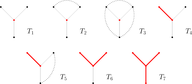
We can apply the technique used in the previous section to count the number of colored partitions for other graphs. Specifically, we enumerate the colored partitions for the product , where , known as the star graph, is defined as in Section 5. Figure 8 illustrates all possible configurations for the last slice of . In this figure, the dotted lines indicate that the two vertices they connect belong to the same block, which is determined by a path that passes through other slices of the graph.
The relations between the variables , which represent the bivariate generating functions for the -colored partitions ending in the configuration , can be encoded in the following matrix:
For example, consider the entry , which corresponds to adding the configuration to , where the last slice is one of six possible configurations . Figure 9 illustrates all six possible configurations. The generating function corresponding to these configurations is given by
Let . Using the matrix , the problem can be formulated as solving the system , where is the vector that contains the base cases. To find t, we first compute , where is the identity matrix. Multiplying this inverse matrix by b gives us the generating functions for each one of the last possible slices. Substituting these results into Equation (8) yields the generating function:
| (8) |
Theorem 7.1.
The bivariate generating function for the -colored partitions of the product graph is given by , where
and
Corollary 7.2.
The expected number of blocks when uniformly and independently coloring the graph with vertices using two colors is given by
To count the size of the system of equations for a general enumeration of -colored partitions for the graph based on the last possible slices, we use the function that counts the number of integer partitions of . For a given , the number of different last slices corresponds to the sum of the number of partitions of integers up to . Specifically, the number of equations required to solve the system is given by
The partition function comes from all possible ways to connect points colored the opposite way of the color given to the vertex with degree . For example, for , we have possible last slices shown in Figure 8.
References
- [1] s-m. belcastro. Domino tilings of grids (or perfect matchings of grid graphs) on surfaces. J. Integer Seq. 26 (2023), Article 23.5.6.
- [2] O. Bodini. On the strange kinetic aesthetic of rectangular shape partitions. Pure Math. Appl. (PU.M.A.) 30 (2022), 37–44.
- [3] T. Došlic and L. Podrug. Sweet division problems: from chocolate bars to honeycomb strips and back. Accepted in the American Mathematical Monthly, (2024).
- [4] P. W. Kasteleyn. Dimer statistics and phase transitions. J. Mathematical Phys. 4 (1963), 287–293.
- [5] R. Mansour. Counting clusters in a coloring grid. Discrete Math. Lett. 5 (2021), 20–23.
- [6] J. L. Ramírez and D. Villamizar. Colored random tilings on grids. J. Autom. Lang. Comb. (2024).
- [7] J. L. Ramírez and D. Villamizar. Counting colored tilings on grids and graphs. In: Proceedings of the 13th edition of the conference on Random Generation of Combinatorial Structures. Polyominoes and Tilings (GASCom 2024), Bordeaux, France, 24-28th June 2024. Electron. Proc. Theor. Comput. Sci. (EPTCS) 403 (2024), 164–168.
- [8] J. Richey. Counting clusters on a grid. Undergraduate Honors Thesis. Dartmouth College, 2014.
- [9] N. Rolin and A. Ugolnikova. Tilings by and . RAIRO-Theor. Inf. Appl. 50 (2016), 105–116
- [10] R. P. Stanley. Algebraic Combinatorics: Walks, Trees, Tableaux, and More. Springer, 2013.
- [11] H. N. V. Temperley and M. E. Fisher. Dimer problem in statistical mechanics—an exact result. Philos. Mag. 6 (1961), 1061–1063.