DeltaGNN: Graph Neural Network with Information Flow Control

Abstract

Graph Neural Networks (GNNs) are popular deep learning models designed to process graph-structured data through recursive neighborhood aggregations in the message passing process. When applied to semi-supervised node classification, the message-passing enables GNNs to understand short-range spatial interactions, but also causes them to suffer from over-smoothing and over-squashing. These challenges hinder model expressiveness and prevent the use of deeper models to capture long-range node interactions (LRIs) within the graph. Popular solutions for LRIs detection are either too expensive to process large graphs due to high time complexity or fail to generalize across diverse graph structures. To address these limitations, we propose a mechanism called information flow control, which leverages a novel connectivity measure, called information flow score, to address over-smoothing and over-squashing with linear computational overhead, supported by theoretical evidence. Finally, to prove the efficacy of our methodology we design DeltaGNN, the first scalable and generalizable approach for detecting long-range and short-range interactions. We benchmark our model across 10 real-world datasets, including graphs with varying sizes, topologies, densities, and homophilic ratios, showing superior performance with limited computational complexity. The implementation of the proposed methods are publicly available at https://github.com/basiralab/DeltaGNN.

I Introduction

GNNs are machine learning models designed to process graph-structured data [1]. They have proven effective in various graph-based downstream tasks [2, 3], especially in semi-supervised node representation learning  [4]. GNNs also demonstrate broad applicability across several distinct domains, including chemistry  [5, 6], and medical fields  [7], such as network neuroscience  [8], and medical image segmentation for purposes such as liver tumor and colon pathology classification [9].

The strength of GNN models lies in their ability to process graph-structured data and capture short-range spatial node interactions through local neighborhood aggregations during message passing. However, such local aggregation paradigm often struggles to capture dependencies between distant nodes, particularly in certain graph densities and structures. For instance, when processing a strongly clustered graph, a standard GNN model may fail to account for interactions between nodes in distant clusters. These long-range interactions (LRIs) are crucial for node classification tasks, as they help distinguish between different classes and improve classification accuracy. This limitation has been widely studied, with theoretical findings pinpointing over-smoothing [10] and over-squashing [11] as the root causes. These phenomena limit performance in many applications and prevent the use of deep GNNs to effectively capture long-range dependencies.

To address these challenges, recent works have proposed enhanced GNN models by integrating graph transformer-based modules, such as global attention mechanisms [12], or local-global attention [13]. Other works have proposed topological pre-processing techniques, such as curvature-enhanced edge rewiring [14] and sequential local edge rewiring [15]. Although these methods can marginally improve model performance, they fail to provide a generalized and scalable approach that can effectively process large graphs across various graph topologies. Specifically, attention-based approaches are constrained by their quadratic time complexity and lack of topological awareness, which leads to computational inefficiency. Rewiring algorithms, on the other hand, rely on expensive connectivity measures that are often impractical for large and dense graphs. These methods are also embedding-agnostic and, consequently, fail to directly address over-smoothing in certain graph structures. For these reasons, developing a scalable and general method for learning long-range interactions (LRIs) would significantly expand the applicability of GNNs in semi-supervised node classification tasks. Such a method would be a key contribution to the field.

In this work, we formalize the concept of graph information flow and use it to define a novel connectivity measure that analyzes the velocity and acceleration of node embedding updates during message passing, offering insights into graph topology and homophily. We provide both theoretical and empirical evidence to support this claim. Next, we propose a new graph rewiring paradigm, information flow control, which mitigates both over-smoothing and over-squashing with minimal additional time and memory complexity. Furthermore, we introduce a novel GNN architecture, DeltaGNN, which implements information flow control to capture both long-range and short-range interactions. We benchmark our model across a wide range of real-world datasets, including graphs with varying sizes, topologies, densities, and homophilic ratios. Finally, we compare the results of our approach with popular state-of-the-art methods to evaluate its generalizability and scalability.

Our contributions. (1) We introduce a novel connectivity measure, the information flow score, which identifies graph bottlenecks and heterophilic node interactions, supported by both theoretical and empirical evidence of its efficacy. (2) We propose an information flow control mechanism that leverages this measure to perform sequential edge-filtering with linear computational overhead, which can be flexibly integrated into any GNN architecture. (3) We design a scalable and generalizable framework, DeltaGNN, for detecting both short-range and long-range interactions, demonstrating the effectiveness of our theoretical findings.

II Preliminaries

A graph is usually denoted as $\mathcal{G}=(\mathcal{V},\mathcal{E})$, where $\mathcal{V}$ represents the node set and $\mathcal{E}$ the edge set. The edge set can also be represented as an adjacency matrix, defined as $\boldsymbol{A}\in\{0,1\}^{|\mathcal{V}|\times|\mathcal{V}|}$, where $\boldsymbol{A}_{ij}\neq 0$ if and only if the edge $(i,j)$ exists. The node feature matrix is defined as $\boldsymbol{X}\in\mathbb{R}^{|\mathcal{V}|\times d_{\mathcal{V}}}$ for some feature dimensions $d_{\mathcal{V}}$. We denote $\boldsymbol{X}^{t}_{u}$ as the features of the node $u$ at layer $t$, with the convention $\boldsymbol{X}^{0}=\boldsymbol{X}$. Furthermore, each node $u$ is associated with a class $y_{u}\in\mathcal{C}$, where $\mathcal{C}$ denotes the set of classes. The goal, in node-classification tasks, is to learn $\Phi:\mathcal{V}\rightarrow\mathcal{C}$, the unique function mapping each node to a specific class.

II-A Graph Neural Networks

Each layer of the GNN applies a transformation function and message-passing aggregation function to each feature vector $\boldsymbol{X}_{u}$ and its neighborhood $\mathcal{N}(u)$. The general formulation of this operation can be expressed as follows:

$$\boldsymbol{X}^{t+1}_{u}=\phi\left(\bigoplus_{v\in\tilde{\mathcal{N}}(u)}\psi(\boldsymbol{X}^{t}_{v})\right)\quad\text{for }0\leq t\leq T$$ (1)

where $\phi$ and $\psi$ are differentiable functions, $\oplus$ is an aggregation function (typically sum, mean, or max), $\tilde{\mathcal{N}}(u)=\mathcal{N}(u)\cup u$ the extended neighbourhood of $u$, and $T$ is the number of layers of the model.

II-B Over-smoothing and Homophily

Over-smoothing [16] can be formalized as follows.

Definition II.1 (Over-smoothing).

Over-smoothing refers to the phenomenon where the representations of nodes become indistinguishable as the number of layers $T$ increases, weakening the expressiveness of deep GNNs and limiting their applicability. In node classification tasks, over-smoothing can hinder the ability of GNNs to distinguish between different classes, as their feature vectors converge to a fixed value with increasing layers:

$$\sum_{(u,v)\in\mathcal{E}:\Phi(u)\neq\Phi(v)}||\boldsymbol{X}^{T}_{u}-\boldsymbol{X}^{T}_{v}||\rightarrow 0\text{ as }T\rightarrow\infty$$

Over-smoothing is accelerated by the presence of edges connecting distinct node classes [17], these are called heterophilic edges. The tendency of a graph to lack heterophilic connections is termed homophily. This property can be quantified by calculating the graph homophilic ratio $\mathcal{H}\in[0,1]$, which is the average of the homophilic ratios of its nodes.

Definition II.2 (Homophilic Ratio of a Node).

The homophilic ratio $\mathcal{H}_{u}\in[0,1]$ of a node $u$ is the proportion of neighbours $u^{\prime}\in\mathcal{N}(u)$ such that $u$ and $u^{\prime}$ belong to the same class. The homophilic ratio is defined as:

$$\mathcal{H}_{u}=\frac{|\{v\in\mathcal{N}(u)\mid\Phi(v)=\Phi(u)\}|}{|\mathcal{N}(u)|}$$

Over-smoothing can be mitigated by increasing graph homophily, for instance, by removing heterophilic edges.

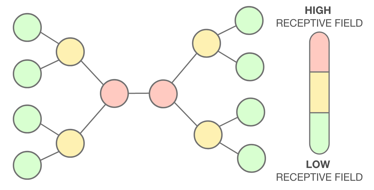
Figure 1: Illustration of a graph with a bottleneck.

II-C Over-squashing and Connectivity

Over-squashing [11], on the other hand, is the inhibition of the message-passing capabilities of the graph caused by graph bottlenecks.

Definition II.3 (Over-squashing).

Over-squashing refers to the exponential growth of a node’s receptive field, leading to the collapse of substantial information into a fixed-sized feature vector due to graph bottlenecks (see Figure 1).

To alleviate over-squashing, it is necessary to improve the connectivity of the graph. This can be achieved by removing or relaxing graph bottlenecks that hinder connectivity [18]. Typically, these bottlenecks can be identified by computing a connectivity measure, such as the Ollivier-Ricci curvature [19, 20] or a centrality measure. The term connectivity measure refers to any topological or geometrical quantity that captures how easily different pairs of nodes can communicate through message passing.

II-D Welford’s Method for Calculating Average and Variance

Welford’s method [21] provides a numerically stable and incremental approach to compute mean and variance. This method is particularly advantageous in scenarios where data points are received sequentially, and real-time updates to the statistics are required. Given a sequence of numbers $x_{1},x_{2},\ldots,x_{n}$, Welford’s method calculates the mean $\mu_{n}$ and variance $\sigma_{n}^{2}$. The mean after $n$ elements can be updated incrementally by:

$$\mu_{n}=\mu_{n-1}+\frac{x_{n}-\mu_{n-1}}{n}$$ (2)

where $\mu_{n}$ is the mean after the first $(n)$ elements. The variance after $n$ elements can be updated using the following formula:

$$\sigma_{n}^{2}=\sigma_{n-1}^{2}+\frac{(x_{n}-\mu_{n-1})\times(x_{n}-\mu_{n})-\sigma_{n-1}^{2}}{n}$$ (3)

where $\sigma_{n}^{2}$ is the variance after the first $n$ elements.

III Related Works

Transformer-based self-attention. A common approach to overcome over-smoothing and over-squashing and capture long-range node interactions is integrating a transformer-based components into the GNN [22, 23, 13, 12]. Transformers can aggregate information globally without being limited by the local neighborhood aggregation paradigm, making them a very effective solution. However, they fail to propose a scalable solution which can process large-scale graphs, which is arguably the scenario where long-range interaction detection is of the utmost importance. Graph self-attention has a time complexity of $O(|\mathcal{V}|^{2})$, where $|\mathcal{V}|$ refers to the number of nodes in the graph, this complexity is unsuitable for large graphs. Moreover, classical transformers are inefficient at processing LRIs in graphs because they are inherently topology-agnostic and consequently process all $|\mathcal{V}|^{2}$ possible interactions.

Topological graph rewiring. Many rewiring algorithms exploit graph curvature [14] or other connectivity measures [15, 24, 25, 26] to identify parts of the graph suffering from over-squashing and over-smoothing, and alleviate these issues by adding or removing edges. Such approaches have two main limitations: first, they rely on expensive connectivity measures (e.g., Ollivier-Ricci curvature, betweenness centrality); and second, they are embedding-agnostic, as they primarily base rewiring decisions on the graph’s connectivity. However, over-smoothing is not a topological phenomenon, and as observed by recent works [27], its effects can be mitigated by acting on the graph’s heterophily. Therefore, improving connectivity alone is insufficient to prevent over-smoothing (see Appendix A).

IV Information Flow

IV-A Graph Information Flow

We define Graph Information Flow (GIF) as the exchange of information between nodes during the message-passing process. This can be quantified as the rate at which node embeddings are aggregated across each layer of the GNN. To observe how GIF changes over time within our model, we introduce two sequences that are useful for quantifying this variation. Let $M$ be a smooth manifold equipped with a distance function $d:M\times M\rightarrow\mathbb{R}$ that defines the geometry of the space. Additionally, assume the features embeddings $\mathbf{X}$ of the input graph lie on $M$.

Definition IV.1 (First Delta Embeddings).

Let $\mathbf{M}_{u}^{t}=\psi(\mathbf{X}_{u}^{t-1})$ be the transformed feature vector of node $u$ at layer $t$. We define the first delta embeddings at layer $t$ as the distance between the aggregated and transformed feature vectors.

$$\Delta^{t}_{u}=d(\bigoplus_{v\in\mathcal{N}(u)}\mathbf{M}_{v}^{t},\mathbf{M}_{u}^{t})\quad\text{for }1\leq t\leq T$$

Where $T\in\mathbb{N}$ defines the number of layers of the architecture. This quantity can be interpreted as the velocity at which the node embeddings are aggregated at layer $t$.

Definition IV.2 (Second Delta Embeddings).

Similarly, let $\Delta^{t}_{u}$ be the first delta embedding of a node $u\in\mathcal{V}$ at time $t\in[1,T]$, where $T\in\mathbb{N}$ defines the number of layers of the architecture. Then, we define the second delta embeddings as the first differences of the first delta embeddings over time.

$$(\Delta^{2})^{t}_{u}=d(\Delta^{t}_{u},\Delta^{t-1}_{u})\quad\text{for }2\leq t\leq T\quad\text{and }\quad(\Delta^{2})^{1}_{u}=0$$

This can be interpreted as the rate of change in the rate at which node embeddings are aggregated within the model, analogous to acceleration in physical systems.

We now provide theoretical evidence showing how the sequences $\Delta^{t}_{u}$ and $(\Delta^{2})^{t}_{u}$ can offer insights into the graph’s homophily and topology, respectively.

Lemma 1.

Let $\Delta^{t}_{u}$ be the first delta embeddings of a node $u$ and $\overline{\Delta_{u}}$ be the average over time of the sequence. Assume $\Delta^{t}_{u}$ converges to zero, $M$ is compact and that there exists a unique function $\phi:M\rightarrow C$ which correctly assign all possible feature vectors to their associated labels. Then, for any homophilic ratio $\mathcal{H}\in[0,1]$, there exists a positive lower-bound $\rho\in(0,+\infty)$ such that any node $u\in\mathcal{V}$ with feature vector $\mathbf{X}_{u}\in M$ and $\overline{\Delta_{u}}>\rho$ will have $\mathcal{H}_{u}<\mathcal{H}$.

Proof.

To prove the lemma, we first show that there exists $\rho$, which is a valid positive lower-bound for every $\Delta_{u}^{t}$ for some node $u$. Then, we deduce that $\rho$ is also a valid lower bound for $\overline{\Delta_{u}}$.

For any node $u\in\mathcal{V}$ within the graph, with feature vector $\mathbf{X}_{u}^{t}\in M$, homophilic ratio $\mathcal{H}_{u}$, and neighbourhood $\mathcal{N}(u)=\{n_{1},n_{2},...,n_{k}\}$ of degree $k$, we define $S$ as the family of all feature assignments $s:\mathcal{N}(u)\rightarrow M$ mapping each neighboring node of $u$ to a feature vector in $M$ such that the following constraint is respected:

$$\mathcal{H}_{u}=\frac{|\{m\in s(v)\textbf{ : }v\in\mathcal{N}(u))\mid\Phi(m)=\Phi(\mathbf{X}_{u}^{t})\}|}{k}$$

Here, the constraint ensures that the feature assignment respects the given homophily ratio $\mathcal{H}_{u}$. Thanks to the existence of $\Phi$ we know that the cardinality of $S$ is at least one, since we can always define $S\ni\tilde{s}(n_{i})=\mathbf{X}_{n_{i}}^{t}\textbf{ }\forall\textbf{ }i\in[1,k]$, where $\mathbf{X}_{n_{i}}^{t}$ are columns of the feature matrix $\mathbf{X}^{t}$ associated to the neighbouring nodes $n_{i}$. In this case, the constraint reduces to the definition of homophilic ratio of $u$. Now, we proceed by defining $\Delta_{u}^{t}$ with respect to a feature assignment $s\in S$ as $\tilde{\Delta_{u}^{t}}(s):=d(\bigoplus_{v\in\mathcal{N}(u)}s(v),\mathbf{M}_{u}^{t})$ for which $\tilde{\Delta_{u}^{t}}(\tilde{s})=\Delta_{u}^{t}$ holds. Since our manifold $M$ is compact, the Hopf–Rinow Theorem [28] ensures that the distance metric $d$ is continuous, which also implies that our $\tilde{\Delta_{u}^{t}}(s)$ is continuously defined for any feature assignment. By the Extreme Value Theorem [29] and the fact that the set $S$ is non-trivial, $\tilde{\Delta_{u}^{t}}(s)$ must attain its maximum real value for some feature assignment $s\in S$. As a result, for any node $u$ with a certain homophilic ratio $\mathcal{H}_{u}$ we can define the real positive constant $U(\mathcal{H}_{u})_{u}:=\sup_{s\in S}\tilde{\Delta_{u}^{t}}(s)$ as the maximum value that the first delta embeddings at time $t$ can take for any possible feature assignment.

Now, for any homophilic ratio $\mathcal{H}\in[0,1]$ we can choose a $\rho>\sup_{h\in[\mathcal{H},1]}U(h_{u})_{u}$ such that any node $u$ with $\Delta^{t}_{u}>\rho$ will have $\mathcal{H}_{u}<\mathcal{H}$. This last implication can be verified assuming, for the sake of contradiction, that the node $u$ may have $\Delta^{t}_{u}>\rho$ and $\mathcal{H}_{u}\geq\mathcal{H}$, and observing that this leads to the following contradiction:

$$\rho<\tilde{\Delta_{u}^{t}}(\tilde{s})\leq\sup_{s\in S}\tilde{\Delta_{u}^{t}}(s)=U(\mathcal{H}_{u})_{u}\leq\sup_{h\in[\mathcal{H},1]}U(h_{u})_{u}<\rho$$

Since this relation holds true for any $t$, we can deduce:

$$\Delta^{t}_{u}>\rho\rightarrow\sum_{i\in[1,T]}\Delta^{i}_{u}>T\rho\rightarrow\overline{\Delta_{u}}>\rho$$

where the penultimate inequality holds if and only if the series is convergent, completing the proof. ∎

In practice, this generalization over the mean helps reduce noise that may affect the first layers. The value of $\rho$ depends on the maximum distance between the subspaces of $M$ associated with the node classes. In some domains, lower thresholds can be obtained, allowing for better distinction between nodes with different homophilic ratios. Finally, since the node classes are hidden from the model, we cannot directly compute the threshold $\rho$. However, it is sufficient to know that, since $\rho$ exists, the nodes with the highest values of $\overline{\Delta}$ will likely have the lowest homophilic rates.

Lemma 2.

Let $c:\mathcal{V}\rightarrow\mathbb{R}$ be a node connectivity measure, and let $\mathbb{V}_{t}[\Delta^{2}_{u}]$ denote the variance over time of the second delta embeddings of a node $u$. Assume that there exists an upperbound $\mu$ such that for any node $u\in\mathcal{V}$, $c(u)<\mu$ if and only if the node $u$ is adjacent to an edge bottleneck. Then, any node $u\in\mathcal{V}$ for which $c(u)<\mu$ will exhibit a low value of the variance $\mathbb{V}_{t}[\Delta^{2}_{u}]$.

Proof.

Recently, [14] demonstrated that nodes adjacent to bottlenecked edges are less affected by over-smoothing, while nodes located in dense areas of the graph experience faster convergence of their vector embeddings. To prove the lemma, we extend these results by observing that $\mathbb{V}_{t}[\Delta^{2}_{u}]$ can be used to classify a node $u$ into one of these two categories.

This observation stems from the definition of over-squashing. Building on the results of [14], we can formalize the correlation between over-squashing and connectivity as follows: for a pair of nodes $u$ and $v$ with feature vectors $\mathbf{X}_{u}^{t}$ and $\mathbf{X}_{v}^{t}$, respectively, where $c_{u}<\mu<c_{v}$ (with $c_{u}$ and $c_{v}$ representing their respective connectivity), and assuming both nodes are equidistant from their neighborhood (implying the same amount of information is aggregated at time $t=1$), we have $\Delta_{v}^{t}\in o(\Delta_{u}^{t})$ (in the little-o notation). In other words, node $v$ experiences faster convergence compared to node $u$, as nodes near bottlenecks tend to have constrained communication paths in the graph and are consequently less likely to experience significant fluctuations in their embedding values. Now, we can distinguish the two cases: $v$ will converge faster, leading to high values of $(\Delta^{2}_{v})^{t}$ for small values of $t$ and low values later in time. On the other hand, for node $u$, the values of $(\Delta^{2}_{u})^{t}$ will vary more slowly over time due to its slower convergence. This intuitive observation implies that $\mathbb{V}_{t}[\Delta_{v}^{2}]$ must necessarily be greater than $\mathbb{V}_{t}[\Delta_{u}^{2}]$.

This concludes the proof, as we have shown that a node with a low connectivity measure (or, equivalently, a bottlenecked node) exhibits a relatively low variance of the second delta embeddings compared to other nodes in the graph.

∎

We would like to discuss one more point: What happens when we compare nodes belonging to very different neighborhoods? When our assumption of the same distance w.r.t. the neighborhoods is not respected, additional noise is introduced into the process, and the convergence of the sequence $\Delta_{v}^{u}$ will also depend on other factors, such as node homophily or feature separability. In these cases, it is evident that our approach will not deterministically find the optimal solution and its accuracy will be negatively affected by the amount of noise introduced. To address this, we implement design choices aimed at reducing the impact of noise and perform numerical experiments to assess its effectiveness (see VI-C).

IV-B Information Flow Score

While over-squashing is a topological phenomenon caused by graph bottlenecks, over-smoothing is worsened due to the presence of heterophilic node interactions. Motivated by our ultimate goal of mitigating these phenomena, and building on the results of Lemmas 1 and 2, we define a node connectivity measure, called the information flow score (IFS), which is minimized for nodes near bottlenecks with a low homophilic ratio (see Equation 4). Consequently, nodes with low values of this measure are likely to correspond to regions where over-smoothing and over-squashing may occur.

$$\textbf{S}_{u}=\frac{m*\mathbb{V}_{t}[\Delta^{2}_{u}]+1}{l*\overline{\Delta_{u}}+1}$$ (4)

Where ($l$ and $m$) are two multipliers that adjust the weight of the mean and variance in the score, respectively. We now explain the rationale behind the definition of the information flow score. From Lemma 1, we know that a high value of $\overline{\Delta}$ is likely to be associated with a low homophilic ratio, and from Lemma 2, a low $\mathbb{V}_{t}[\Delta^{2}]$ indicates proximity to an edge bottleneck. Consequently, the score is defined as a fraction involving these two terms. Since, in some applications, we may prioritize detecting bottlenecks over heterophilic edges (or vice versa), we introduce the two multipliers $l$ and $m$. In our case, we aim to detect both with equal priority, so we set $m=1$ and $l=1$. To ensure the score remains well-defined, regardless of the delta values, and to prevent it from exploding when the deltas are close to zero, we add 1 to both the numerator and denominator. An additional advantage of adding 1 is that isolated nodes will receive a score of one, which is relatively low. As a result, training the model to rewire the graph while maximizing the overall score will encourage the model to remove edges while still preserving sparsity. To reduce the impact of noise affecting the initial delta values, both the variance and mean are computed using an exponential moving average, which assigns greater weight to more recent data points.

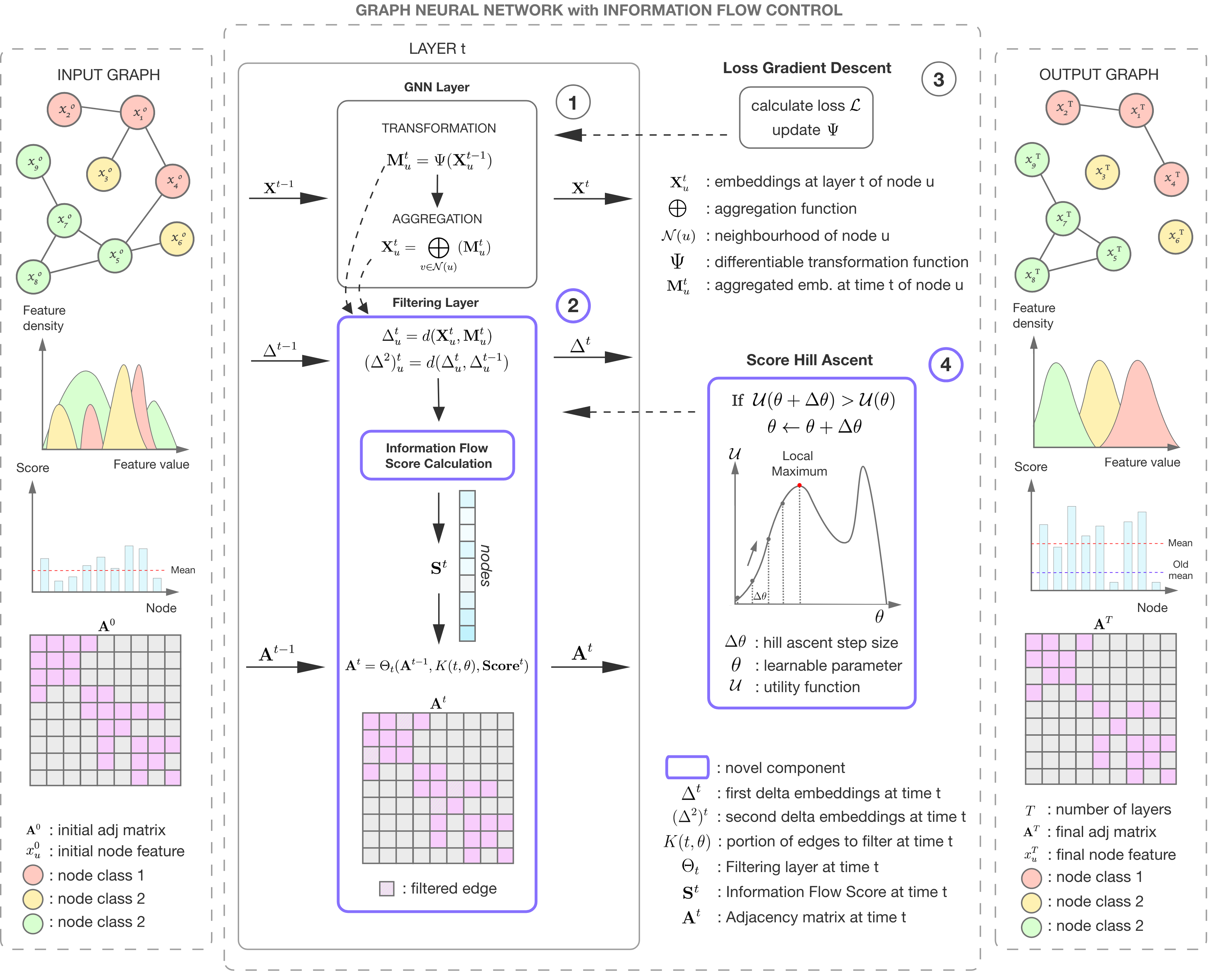
Figure 2: Overview of a GNN model with information flow control. The figure illustrates how the information flow control mechanism integrates with a standard GNN to filter the graph and increase the mean node score. Simultaneously, the GNN learns to disentangle the node features, ensuring that the output embeddings can be easily classified using a readout layer. The novel components are highlighted in violet. Notably, the mean node score of the processed graph is significantly higher due to the effective edge filtering performed within the GNN layers.

IV-C Information Flow Control

Now, we present how to integrate the IFS into a generic GNN to prevent over-smoothing and over-squashing. While common connectivity measures are typically calculated before transforming the graph, our score is computed during the graph transformation learning. Therefore, standard approaches such as graph-rewiring algorithms are not well-suited for handling our measure. To address this limitation, we designed a novel method called information flow control (IFC) (see Figure 2). We first introduce some notations and then propose the novel components of the IFC. We define a topological edge-filtering operation as a function $\Theta(\mathcal{G},K(\theta),c)$ returning a filtered graph $\mathcal{G}^{\prime}$, where $K(\theta)\in[0,1]$ is a $\theta$-parameterized function defining the percentage of edges which has to be removed and $c\in\mathbb{R}^{|\mathcal{V}|}$ are the nodes connectivity values used to choose which edges to remove. The IFC is composed of a sequence of $T$ flow-aware edge-filtering layers $\{\Theta_{t}\}_{t}$ that iteratively filter the graph $\mathcal{G}$:

$$\mathcal{G}=\mathcal{G}_{0}\xrightarrow[]{\Theta_{1}}\mathcal{G}_{1}\xrightarrow[]{\Theta_{2}}\mathcal{G}_{2}\ldots\xrightarrow[]{\Theta_{T}}\mathcal{G}_{T}$$

Each filtering operation is defined as $\Theta_{t}(\mathcal{G}_{t-1},K(t,\theta),\mathbf{S}^{t})$, where $\mathbf{S}^{t}\in\mathbb{R}^{|\mathcal{V}|}$ is the IFS of the graph nodes calculated on the deltas up to layer $t$. These filtering layers are interwoven with standard GNN layers $\{\Omega_{t}\}_{t}$, which are responsible to aggregate and transform the node representations.

$$(\mathbf{A}^{0},\mathbf{X}^{0})\xrightarrow[]{\Omega_{1}}(\mathbf{A}^{0},\mathbf{X}^{1})\xrightarrow[]{\Theta_{1}}(\mathbf{A}^{1},\mathbf{X}^{1})\ldots\xrightarrow[]{\Theta_{T}}(\mathbf{A}^{T},\mathbf{X}^{T})$$

Where $\mathbf{A}^{t}$ denotes the adjacency matrix of $\mathcal{G}$ at layer $t$. The IFC also includes a component that maximizes the mean node score by optimizing the parameter $\theta$ through hill ascent over a utility function $\mathcal{U}$. We set an initial value of zero for $\theta$ and perform a local hill ascent to find a local maximum. This approach is advantageous because the IFC is encouraged to preserve sparsity, increasing the number of edges removed only if it leads to an increase in the utility function $\mathcal{U}$ (e.g., the mean of the scores at the last layer). Follows a pseudo-code implementing the forward-pass of a GNN with our IFC module.

Algorithm 1 GNN with IFC: forward-pass

1:Input: Node features $\mathbf{X}^{0}$, adjacency matrix $\mathbf{A}^{0}$, Previous utility value $\mathcal{U}_{old}$

2:Output: Processed features $\mathbf{X}^{T}$, updated adjacency matrix $\mathbf{A}^{T}$

3:Initialize variable $\Delta^{0}=0$, score array $\mathbf{S}$, $\theta=0$

4:for each layer $t$ do

5:  Compute transformed features $\mathbf{M}^{t}$$\triangleright$ (1)

6:  Compute $\mathbf{X}^{t}$ by aggregating $\mathbf{M}^{t}$$\triangleright$ (1)

7:  Compute $\Delta^{t}$$\triangleright$ (IV.1)

8:  if not first layer then

9:   Compute $(\Delta^{2})^{t}$$\triangleright$ (IV.2)

10:  else

11:   Set $(\Delta^{2})^{t}=0$

12:  end if

13:  Update $\overline{\Delta^{t}}$ applying Welford’s Method on $\overline{\Delta^{t-1}}$ $\triangleright$ (2)

14:  Update $\mathbb{V}[(\Delta^{2})^{t}]$ applying Welford’s Method on $\mathbb{V}[(\Delta^{2})^{t-1}]$ $\triangleright$ (3)

15:  Compute scores $\mathbf{S}^{t}$$\triangleright$ (4)

16:  Update $\mathbf{A}^{t}$ removing $K(t,\theta)$ edges with low IFS from $\mathbf{A}^{t-1}$

17:end for

18:Compute utility value $\mathcal{U}_{new}$ based on final scores $\mathbf{S}^{T}$ (e.g. mean node score)

19:if $\mathcal{U}_{new}>\mathcal{U}_{old}$ then

20:  Update parameter $\theta$ with step size $\Delta\theta$ (hill ascent step)

21:end if

22:return processed features $\mathbf{X}^{T}$, updated adjacency matrix $\mathbf{A}^{T}$, new utility value $\mathcal{U}_{new}$

V Methodology: DeltaGNN

In this section, we illustrate DeltaGNN and how it leverages the IFC to capture both short-range and long-range node interactions overcoming the limitations of its predecessor [30]. First, DeltaGNN processes the node embeddings and graph adjacency matrix through a standard homophilic GNN with IFC. During the sequential filtering, the model partitions the graph into homophilic clusters by removing bottlenecks and heterophilic edges. Simultaneously, the homophilic aggregation learns short-range dependencies. However, this process leads to the loss of long-range interactions, which we recover through an heterophilic graph condensation. The long-range dependencies are then learned via a GNN heterophilic aggregation. Finally, a readout layer processes the results from both GNN aggregations. An overview of the model pipeline is illustrated in Figure 3.

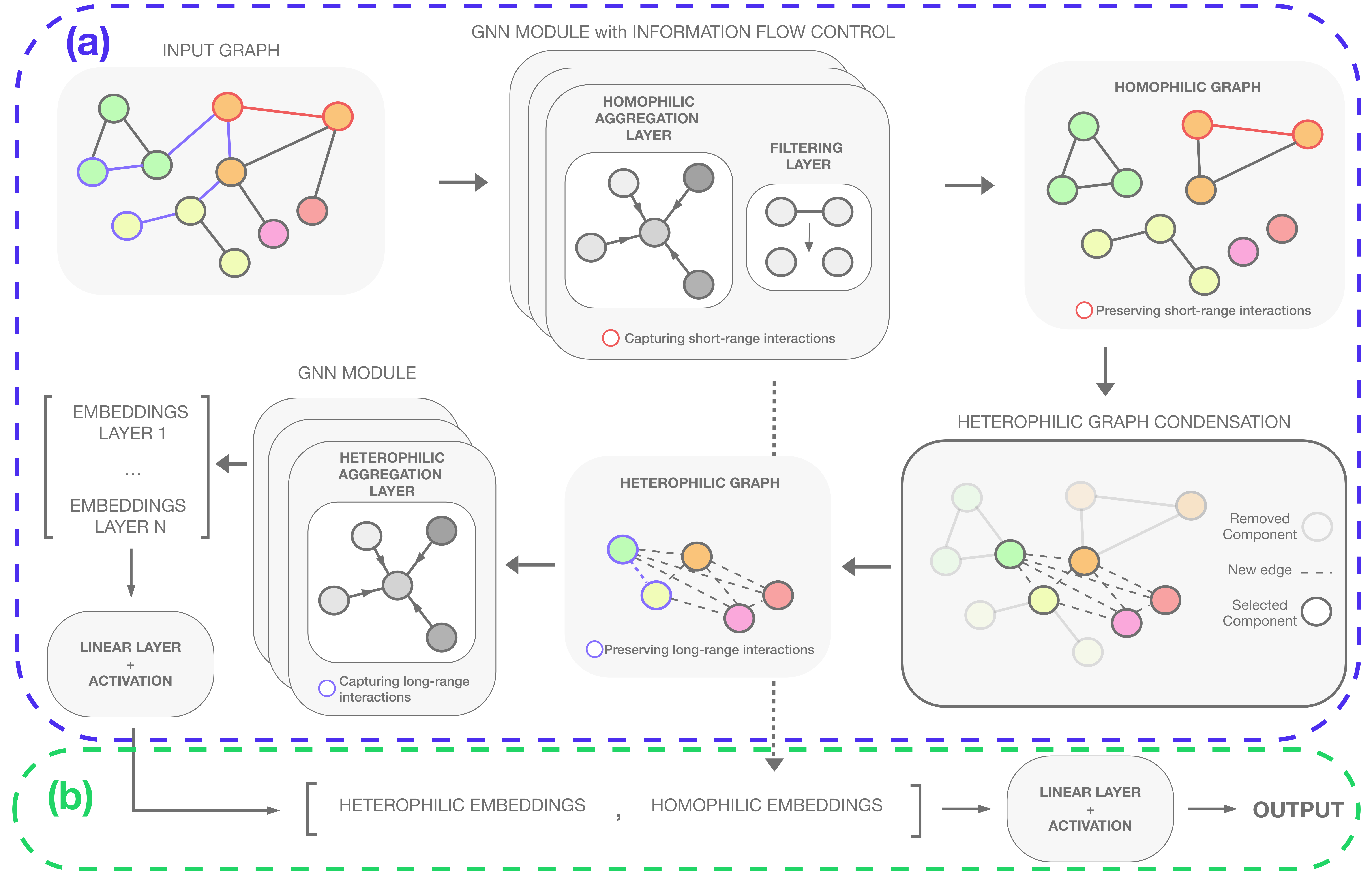
Figure 3: The DeltaGNN pipeline consists of: (a) a sequential transformation stage that processes both homophilic and heterophilic edge interactions, performing homophily-based interaction-decoupling and dual aggregation to learn short-term and long-term dependencies; and (b) a prediction stage that concatenates the results from the first stage.

V-A Sequential transformation stage

The sequential transformation stage includes a homophilic aggregation with IFC, a heterophilic graph condensation, and a heterophilic aggregation. This stage is designed to discriminate between homophilic and heterophilic node interactions, producing a strongly homophilic graph and a strongly heterophilic graph, which are processed by independent GNN modules. This concept of homophily-based interaction-decoupling is crucial to prevent over-smoothing by avoiding using a standard GNN aggregation on heterophilic edges. During the homophilic aggregation (see Equation 1) the model capture short-range spatial interactions, while the IFC removes most heterophilic edges within the graph, breaking it into homophilic connected components (see Figure 3). We set $\mathcal{U}=\overline{\mathbf{S}^{T}}$ and the step size $\Delta\theta=\eta$, where $\eta$ denotes the learning rate of the transformation function of the GNN module. At each GNN layer $t$, we remove the $K(t,\theta)$ edges with the lowest scores, which are calculated using the Euclidean distance $d(\mathbf{x},\mathbf{y})=\|\mathbf{x}-\mathbf{y}\|$. This process reduces over-smoothing by increasing the homophily of the graph, and over-squashing, by removing the graph bottlenecks. As a result, the output graph of this first step, which we define $\mathcal{G}_{\textit{ho}}$, will be highly homophilic and preserve most short-term node interactions. On the other hand, most long-range interaction will be lost during the edge filtering.

Next, we proceed with the heterophilic graph condensation, which aims at extracting the most relevant heterophilic interactions within the homophilic clusters to re-introduce long-range dependencies. To achieve this, we select the nodes with the highest scores, which are likely to have the most reliable representations, and construct a distinct fully-connected graph with them. The resulting graph, defined as $\mathcal{G}_{\textit{he}}$, will be highly heterophilic since nodes with different labels are likely to be neighbours due to the clustering during the score-based edge filtering. This graph will preserve the majority of the LRIs while resulting considerably smaller than the original graph. Next, we apply the heterophilic aggregation on $\mathcal{G}_{\textit{he}}$ which is a simple variation of the standard update rule defined in equation 5.

$$\boldsymbol{X}^{t+1}_{u}=\phi\left(\bigoplus_{v\in\mathcal{N}(u)}\psi(\boldsymbol{X}^{t}_{v}),\psi^{s}(\boldsymbol{X}^{t}_{u})\right),$$

$$\boldsymbol{X}^{1}_{u}=\phi\left(\psi^{s}(\boldsymbol{X}^{0}_{u})\right),\quad\text{for }0\leq t\leq L-1$$ (5)

where $\psi^{s}$ is a differentiable function used to process node self-connections. Additionally, we do not aggregate the node features in the first layer so that the model can process the original features. Finally, we build a row vector of all layers’ node embedding outputs $\mathbf{X}^{i}_{he}$ and feed it into a linear layer, similarly to what was done in [31] (see Equation 6). This ensures that the model learns to distinguish between different node classes at many levels of smoothness.

V-B Prediction stage

In this stage, we concatenate and process both modules’ outputs, $\boldsymbol{X}_{\textit{ho}}^{out}$ and $\boldsymbol{X}_{\textit{he}}^{out}$, through a final linear layer to perform the prediction (see Equation 6).

$$\boldsymbol{X}_{\textit{he}}^{out}=\phi_{\textit{he}}\left(\boldsymbol{W}_{\textit{he}}^{out}\begin{bmatrix}\boldsymbol{X}_{\textit{he}}^{1}\\ \boldsymbol{X}_{\textit{he}}^{2}\\ \vdots\\ \boldsymbol{X}_{\textit{he}}^{T}\end{bmatrix}\right)$$

$$\boldsymbol{X}^{out}=\phi_{\textit{out}}\left(\boldsymbol{W}^{out}\begin{bmatrix}\boldsymbol{X}_{\textit{ho}}^{out}\\ \boldsymbol{X}_{\textit{he}}^{out}\end{bmatrix}\right)$$ (6)

VI Experiments

Here, we evaluate DeltaGNN on 10 distinct datasets with varying homophilic ratios, densities, sizes, and topologies. For all datasets, the hyper-parameter fine-tuning was done using a grid-search on the validation set. We compare our DeltaGNN (implemented using GCN aggregations), with state-of-the-art GNN architectures such as GCN [2], GIN [32], GAT [33], rewiring algorithms [34], heterophily-based methods [35, 36], and graph-transformers [37, 38]. Additional details on dataset details, training settings, and models can be found in the Appendix B.

• Cora, CiteSeer, and PubMed datasets. We evaluate our framework on three scientific publications-citations datasets [39, 40] with high homophilic ratios ($\geq$ 0.5). These datasets include one graph each and the task is node-level multi-class classification across several fields of research.

• Cornell, Texas, and Wisconsin datasets. We also use three webpage network datasets [36] with low homophilic ratios ($\leq$ 0.5). These datasets include one graph each and the task is node-level multi-class classification among several webpage categories.

• MedMNIST Organ-C and Organ-S datasets. The MedMNIST Organ-C and Organ-S datasets [9] include abdominal CT scan images (28 $\times$ 28 pixels) of liver tumors in coronal and sagittal views, respectively. The task for both is node-level multi-class classification among 11 types of liver tumors. Each image-based dataset is converted into a graph, with each node representing an image, and each node embedding being the vectorization of the 28 by 28 pixel intensity, resulting in vectors of length 784. The graph edges are derived from the cosine similarity of the node embeddings, similar to what as done in [41, 42]. To reduce complexity, we sparsify these graphs using a sparsity threshold and convert them into unweighted graphs. Additionally, we define two degrees of density for each dataset, with up to $\sim$2.8 million edges.

TABLE I: Accuracy $\pm$ std over 5 runs on six datasets with varying homophily.

Methods	CORA $\mathcal{H}=0.81$	Citeseer $\mathcal{H}=0.74$	PubMed $\mathcal{H}=0.80$	Cornell $\mathcal{H}=0.30$	Texas $\mathcal{H}=0.09$	Wisconsin $\mathcal{H}=0.19$
GCN [2]	85.12±0.42	76.10±0.32	88.26±0.48	37.84±2.70	70.81±2.96	55.69±2.63
GCN + rewiring(DC)	85.32±0.49	76.36±0.38	88.24±0.40	41.08±1.21	70.81±3.52	56.47±1.64
GCN + rewiring(EC)	84.92±0.52	75.80±0.46	88.24±0.25	50.54±0.00	69.19±4.10	52.16±5.65
GCN + rewiring(BC)	84.82±0.71	75.42±0.62	OOT	37.30±4.44	65.94±5.27	54.90±2.78
GCN + rewiring(CC)	85.06±0.26	75.44±0.51	OOT	37.30±6.45	69.73±2.96	54.90±2.78
GCN + rewiring(FC)	85.12±0.45	75.48±0.60	87.94±0.33	50.54±0.00	67.57±5.06	52.55±3.22
GCN + rewiring(RC)	84.90±0.62	75.94±0.43	OOT	31.35±11.40	71.34±2.42	56.86±4.80
GCN + rewiring(IFS)	85.36±0.21	75.92±0.22	87.66±0.88	50.54±0.00	71.35±1.48	54.51±3.51
GIN [32]	83.84±0.70	72.72±0.73	87.80±0.42	58.38±2.42	56.21±5.86	52.55±0.88
GIN + rewiring(DC)	83.76±0.43	72.84±0.59	87.94±0.64	48.11±7.50	60.54±4.52	53.33±2.15
GIN + rewiring(EC)	84.02±0.85	73.56±0.28	88.20±0.77	50.27±6.22	60.54±3.63	52.94±3.67
GIN + rewiring(BC)	83.66±0.79	73.02±0.58	OOT	55.67±4.10	58.38±4.10	55.29±3.51
GIN + rewiring(CC)	83.60±0.70	72.90±0.99	OOT	55.13±4.91	65.40±4.83	53.72±2.23
GIN + rewiring(FC)	83.16±0.93	73.50±0.84	87.30±0.37	56.22±5.54	58.92±4.83	49.80±2.97
GIN + rewiring(RC)	83.22±0.72	73.32±1.28	OOT	57.84±3.63	61.62±4.44	52.94±2.77
GIN + rewiring(IFS)	82.94±1.00	73.38±1.30	87.90±0.96	54.95±5.86	57.84±1.48	53.33±2.91
GAT [33]	85.42±0.95	78.08±0.26	85.48±0.58	38.38±4.83	64.32±2.26	51.37±1.64
GAT + rewiring(DC)	85.26±0.67	77.82±0.33	85.36±0.52	37.30±4.44	62.16±5.06	50.59±3.51
GAT + rewiring(EC)	85.30±0.87	77.54±0.31	85.34±0.57	38.92±4.52	60.00±5.20	50.59±1.64
GAT + rewiring(BC)	85.46±1.21	78.26±0.50	OOT	38.92±4.52	64.86±4.27	52.16±4.51
GAT + rewiring(CC)	85.50±0.72	78.10±0.59	OOT	37.30±4.83	63.78±3.08	52.16±2.23
GAT + rewiring(FC)	86.00±0.87	77.86±0.77	85.60±0.27	37.30±4.01	58.92±10.71	50.20±4.29
GAT + rewiring(RC)	85.28±0.57	78.64±0.36	OOT	35.13±3.31	62.70±6.73	51.76±1.07
GAT + rewiring(IFS)	85.80±0.40	78.06±0.78	85.02±0.58	35.13±4.27	57.84±11.40	47.84±4.07
MPL [43]	70.32±2.68	68.64±1.98	86.46±0.35	71.62±5.57	77.83±5.24	82.15±6.93
SDRF [34]	86.40±2.10	72.58±0.20	OOT	57.54±0.34	70.35±0.60	61.55±0.86
H2GCN [35]	83.48±2.29	75.16±1.48	88.86±0.45	75.40±4.09	79.73±3.25	77.57±4.11
GEOM-GCN [36]	84.10±1.12	76.28±2.06	88.13±0.67	54.05±3.87	67.57±5.35	68.63±4.92
UniMP [37]	84.18±1.39	75.00±1.59	88.56±0.32	66.48±12.5	73.51±8.44	79.60±5.41
NAGphormer [38]	85.77±1.35	73.69±1.48	87.87±0.33	56.22±8.08	63.51±6.53	62.55±6.22
DeltaGNN - control	84.56±0.57	79.40±0.77	89.64±0.73	75.13±1.21	67.57±2.70	74.12±1.64
DeltaGNN - control + DC	84.60±1.05	79.90±0.79	89.70±0.10	75.67±1.91	72.43±1.21	76.47±1.39
DeltaGNN - control + EC	84.14±0.63	79.36±0.59	89.68±0.47	72.97±3.31	73.51±1.21	74.90±3.22
DeltaGNN - control + BC	84.36±0.57	78.98±0.86	OOT	72.97±1.91	70.81±3.52	74.51±2.77
DeltaGNN - control + CC	84.54±0.93	79.46±0.75	OOT	74.05±1.48	70.81±2.26	75.29±2.97
DeltaGNN - control + FC	84.94±0.75	79.36±0.65	89.98±0.24	73.51±1.21	71.89±1.48	73.33±1.07
DeltaGNN - control + RC	84.96±0.50	79.34±0.59	OOT	74.05±1.48	72.43±1.91	76.08±0.88
DeltaGNN constant	86.38±0.18	79.15±0.43	89.73±0.31	70.27±4.10	74.05±3.08	79.21±1.75
DeltaGNN linear	87.29±0.52	79.42±0.78	89.60±0.45	75.27±3.31	72.97±3.82	80.00±0.88

Notes: Results better than their counterparts have a more intense shade of green. OOT indicates an out-of-time error (compute time $\geq$ 30 mins).

Figure 4: Validation accuracy (red) and specificity (blue) convergence during training epochs for DeltaGNN linear on three datasets with varying homophilic ratios. The dashed line indicates the observed convergence point.

VI-A Generalizability Benchmark

In this section, we assess the efficacy of our models on six datasets with varying homophilic ratios. As most GNNs rely on graph homophily, this experiment helps us gauge our model dependence on this assumption and its generalizability across different domains. As shown in Table I, DeltaGNN outperforms all state-of-the-art methods across four out of six datasets, with an average accuracy increase of 1.23%. When comparing the performance of different connectivity measures, we notice that both topology-based and geometry-based connectivity measures fail to offer a generalizable solution across different homophilic scenarios. On the other hand, DeltaGNN is the only approach that consistently yields the best results, consolidating our claim that the IFS is a one-for-all connectivity measure. Furthermore, while expensive measures such as betweenness centrality (BC), closeness centrality (CC), and Ollivier-Ricci curvature (RC) encountered out-of-time (OOT) errors on the PubMed dataset, our IFS, along with degree centrality (DC), eigenvector centrality (EC), and Forman-Ricci curvature (FC), proved scalable enough to process all six datasets. When analyzing the results obtained from datasets with low homophilic rates, such as Texas and Wisconsin, we observe that the performance gap between DeltaGNN and rewiring approaches increases, demonstrating the effectiveness of IFC in improving the homophilic rate of a graph through iterative edge filtering. A more rigorous experiment on this observation is presented in Section VI-C, where we compare the rate of change of the graph homophilic ratio during the edge filtering using different connectivity measures.

VI-B Scalability Benchmark

DeltaGNN exhibits the lowest epoch time in three out of five datasets, in some cases being up to three times faster than its ablations. The introduction of IFC in DeltaGNN reduced the average epoch time by 30.61% when compared to the worst-performing model (see Table II). However, DeltaGNN shows higher-than-average epoch time on the CiteSeer dataset due to the large size of feature vectors. Additionally, thanks to IFC, DeltaGNN is the only LRI architecture with no preprocessing overhead. In terms of memory consumption, DeltaGNN uses approximately twice the memory of standard GCN models. This is due to its implementation, which employs GCN aggregation layers along with dual homophilic and heterophilic aggregations, inherently requiring more parameters. Nevertheless, GAT showed the highest memory footprint, being the only model that failed to process both dense datasets. Graph-transformers and heterophily-based methods proved to be at least as computationally expensive as GAT, failing to process the largest graphs.

The major advantage of using the IFS lies in its synergy with GNNs. Since all GNNs process the input graph through message-passing, it is possible to calculate the score with almost no additional computational cost, as the score for any node has constant time complexity. The additional overhead for computing the score is $O(|\mathcal{V}|d_{\mathcal{V}}T)$, depending on the distance function used. Typically, we have $T\ll d_{\mathcal{V}}\ll|\mathcal{V}|$, which results in an average time complexity of $O(|\mathcal{V}|)$. To the best of our knowledge, this offers the lowest time complexity among all major connectivity measures proposed in the literature (see Table III).

The memory complexity of the IFS is also linear with respect to the number of nodes, $O(|\mathcal{V}|)$, since both the variance and mean can be computed iteratively using Welford’s method [44], without the need to store all previous delta values.

TABLE II: Computational resource comparison. The best connectivity measure with respect to epoch time is used.

Methods	CORA		CiteSeer
	$\Delta$ GPU Memory	$\Delta$ Epoch Time	$\Delta$ GPU Memory	$\Delta$ Epoch Time
GCN + filtering	-69.99%	-31.62%	-63.49%	-40.90%
GIN + filtering	-25.58%	-30.84%	-30.72%	-40.26%
GAT + filtering	-55.10%	0%	-54.11%	0%
DeltaGNN - control	0%	-19.63%	0%	-33.48%
DeltaGNN	0%	-42.06%	0%	-14.64%

Methods	PubMed		Organ-S
	$\Delta$ GPU Memory	$\Delta$ Epoch Time	$\Delta$ GPU Memory	$\Delta$ Epoch Time
GCN + filtering	-65.68%	-6.69%	-70.65%	-17.27%
GIN + filtering	-52.53%	-6.62%	-60.28%	-17.21%
GAT + filtering	0%	-3.49%	0%	-6.93%
DeltaGNN - control	-16.48%	0%	-30.78%	0%
DeltaGNN	-16.48%	-56.16%	-29.47%	-24.10%

Methods	Organ-S dense
	$\Delta$ GPU Memory	$\Delta$ Epoch Time
GCN + filtering	-57.63%	-41.50%
GIN + filtering	-44.19%	-41.45%
GAT + filtering	OOM	OOM
DeltaGNN - control	-3.20%	0%
DeltaGNN	0%	-16.11%

Notes: The rate of change is calculated relative to the worst-performing variation. Results that outperform their counterparts are shaded with a more intense green. OOM indicates an out-of-memory error.

TABLE III: Time complexity of common connectivity measures [45, 20] and our novel IFC.

Topological Measures	Connectivity Measure	Time Complexity
	Degree Centrality (DC)	$O(|\mathcal{E}|)$
	Eigenvector Centrality (EC)	$O(|\mathcal{V}|+|\mathcal{E}|)$
	Betweenness Centrality (BC)	$O(|\mathcal{V}||\mathcal{E}|)$
	Closeness Centrality (CC)	$O(|\mathcal{V}||\mathcal{E}|)$
Geometrical Measures	Ollivier-Ricci Curvature (OC)	$O(|\mathcal{V}||\mathcal{E}|)$
	Forman-Ricci Curvature (FC)	$O(|\mathcal{E}|)$
Embeddings-Based Measures	Information Flow Score (IFS)	$O(|\mathcal{V}|)$

VI-C Numerical Experiment

We now illustrate how our edge-filtering based on the information flow score can improve the homophily and connectivity of the graph, resulting in an increase in the mean node score. We experiment with a small graph containing fourteen nodes belonging to three distinct classes, including bottlenecked and heterophilic edges. As shown in Figure 6, these edges can be easily detected using the IFS values. We then remove the edges adjacent to the nodes with the lowest scores. The filtered graph, as illustrated in Figure 6, demonstrates higher homophily, fewer bottlenecks, and consequently, a higher mean node score.

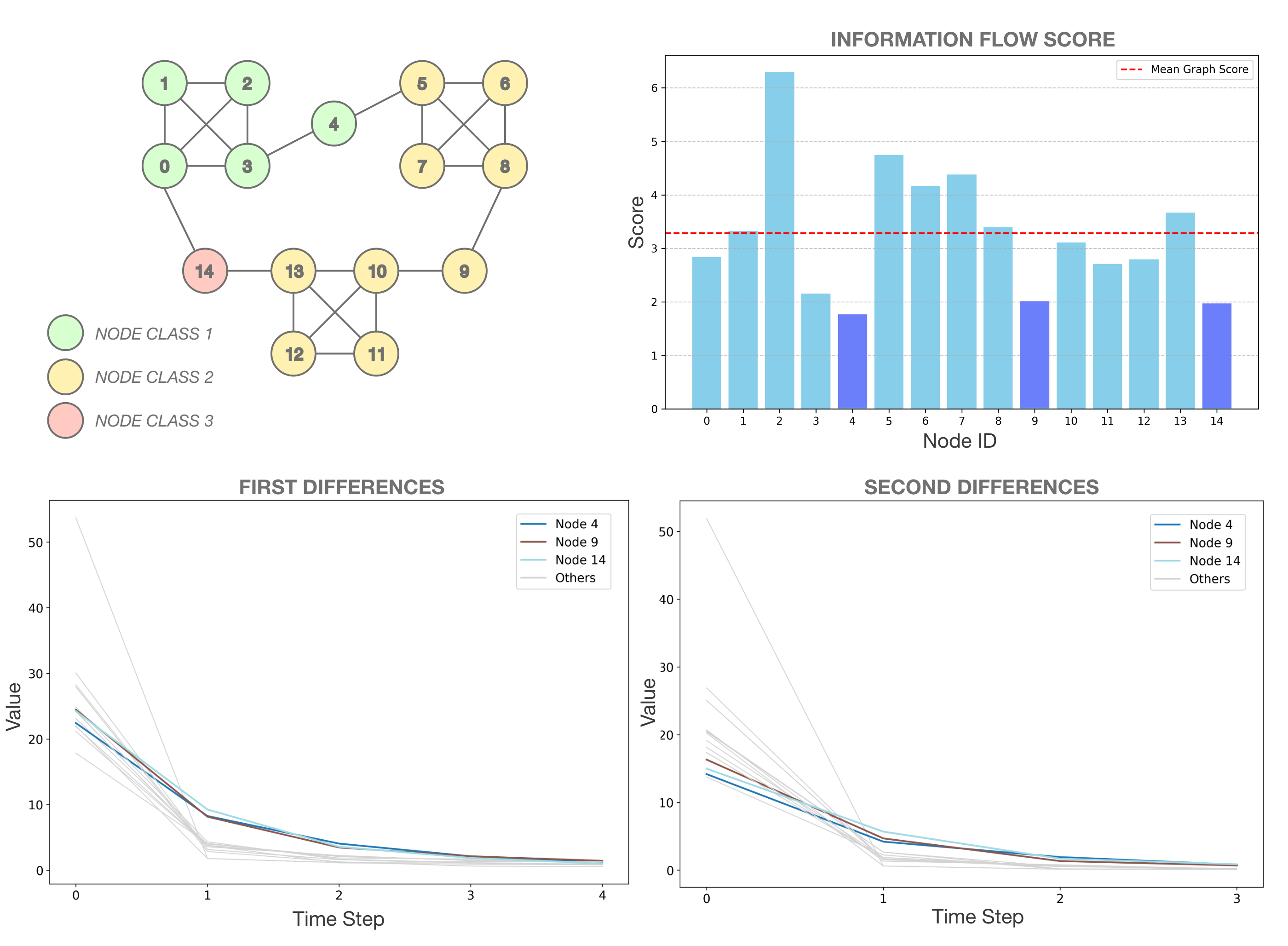
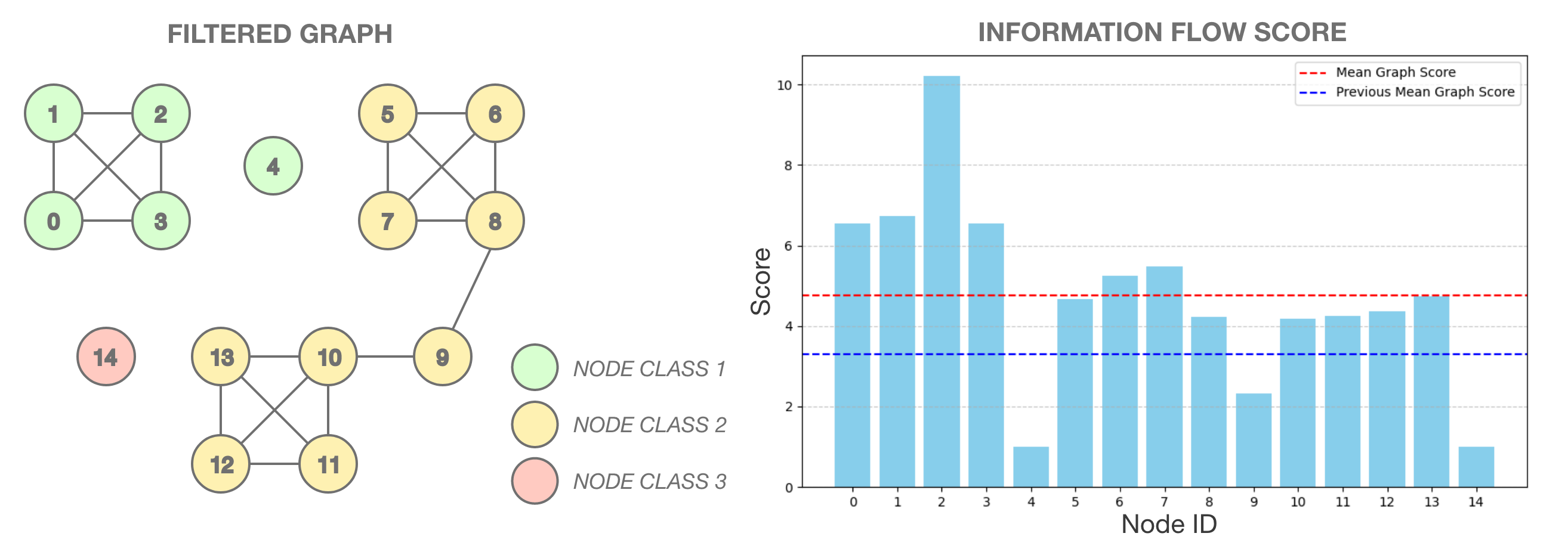
Figure 5: Illustrations of first delta embeddings, second delta embeddings, and information flow score on a small graph with bottlenecks and heterophilic edges. We set $m=1$ and $l=1$ to detect heterophilic bottlenecks, using the Euclidean distance as the distance metric $d$. The samples used to generate the graph are medical images from the MedMNIST Organ-C dataset [9]. As observed from the plots, nodes 4, 9, and 14 can be easily distinguished as they have very low scores.

Figure 6: Filtered graph with updated information flow score. After removing bottleneck edges and heterophilic node interactions, the mean node score increased significantly, demonstrating the effectiveness of the edge filtering.

VI-D Connectivity Measure Comparison

In this section, we directly compare the efficacy of different connectivity measures during topological edge-filtering and heterophilic graph condensation. Figure 7 and Table IV illustrate how the density distribution of the node homophilic rate changes throughout these two stages using various connectivity measures on the CORA dataset. Following the example of recent works [46], we define the homophilic ratio to account for both feature similarity and label similarity to more accurately depict the performance disparity between different methods. Let $e$ be an edge connecting the nodes $u$ and $v$ with feature vectors $\mathbf{X}_{u}$ and $\mathbf{X}_{v}$, respectively. Let $\Phi$ be a function mapping each feature vector to its associated label, and $\delta$ a function returning 1 if the two inputs coincide and 0 otherwise. Then the homophilic rate of $e$ is defined as:

$$\mathcal{H}_{e}=0.5\cdot\frac{\mathbf{X}_{u}\cdot\mathbf{X}_{v}}{\|\mathbf{X}_{u}\|\|\mathbf{X}_{v}\|}+0.5\cdot\delta(\Phi(\mathbf{X}_{u}),\Phi(\mathbf{X}_{v}))$$

where the left term denotes the cosine similarity of the two feature representations.

During topological edge-filtering, the IFS shows the best result, with an increase in the graph homophilic ratio of 8.65%. This demonstrates that our novel connectivity measure is highly effective at reducing over-smoothing and increasing the graph homophily. In contrast, all other embedding-agnostic measures showed significantly worse results, proving that our approach of leveraging the rate of change of the embeddings throughout the message-passing successfully improves the topological edge-filtering. When analyzing the rate of change in the homophilic rate during heterophilic graph condensation, we observe that the IFS yields the lowest variation. The highest rate of change is observed with the Ollivier-Ricci curvature, as illustrated in Figure 7 by the substantial decrease in the number of heterophilic nodes with a homophilic rate close to 0.1 during curvature-based edge filtering. Nevertheless, we can also observe that the performance of betweenness and closeness centrality during heterophilic edge condensation differs substantially. Given their theoretical similarity, this suggests that the role of the connectivity measure in heterophilic graph condensation might be marginal. Therefore, further experiments are needed to determine whether this disparity could impact the model performance.

TABLE IV: Variations in the homophilic rate during topological edge-filtering and heterophilic graph condensation using different connectivity measures.

Methods	CORA
	Original Graph	Homophilic Filtered Graph	$\Delta$ Homophilic Rate	Heterophilic Condensed Graph	$\Delta$ Homophilic Rate
Degree Centrality	0.6676	0.7115	+6.72%	0.981	-85.28%
Eigenvector Centrality	0.6676	0.6937	+4.05%	0.1122	-83.17%
Betweenness Centrality	0.6676	0.7057	+5.85%	0.905	-86.42%
Closeness Centrality	0.6676	0.7043	+5.64%	0.1244	-81.34%
Forman-Ricci Curvature	0.6676	0.7094	+6.40%	0.955	-85.67%
Ollivier-Ricci Curvature	0.6676	0.7112	+6.67%	0.767	-88.49%
Information Flow Score	0.6676	0.7244	+8.65%	0.1560	-76.60%

Notes: Results are bolded if they represent the best performance overall. Results that are better than their counterparts are shaded in progressively darker green.

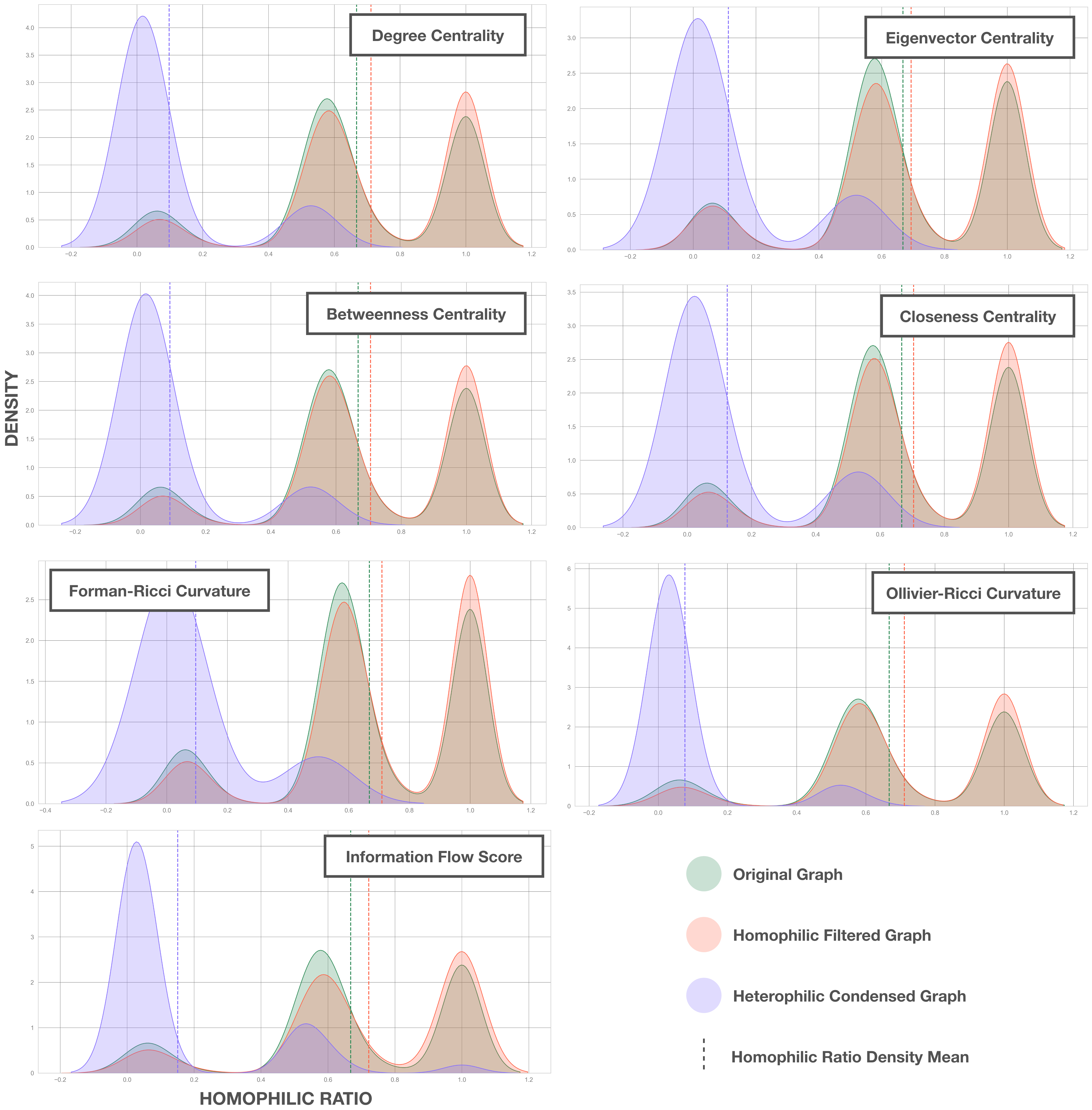
Figure 7: Homophilic ratio density distribution shifts during topological edge-filtering and heterophilic graph condensation using seven distinct connectivity measures. The dashed lines indicate the mean density for each corresponding measure and density.

TABLE V: Prediction result comparison of various methods on four datasets with varying density.

Methods	Organ-S		Organ-S (dense)		Organ-C		Organ-C (dense)
	Accuracy	Specificity	Accuracy	Specificity	Accuracy	Specificity	Accuracy	Specificity
GCN [2]	59.25±0.40	95.92±0.04	57.80±0.41	95.78±0.04	77.25±0.29	97.72±0.03	74.65±0.62	97.46±0.06
GCN + rewiring(DC)	59.02±0.20	95.90±0.02	58.25±0.42	95.82±0.04	76.79±0.29	97.68±0.03	74.92±0.19	97.49±0.02
GCN + rewiring(EC)	58.96±0.44	95.90±0.04	57.94±0.43	95.79±0.04	77.24±0.25	97.72±0.02	75.17±0.31	97.51±0.03
GCN + rewiring(BC)	OOT	OOT	OOT	OOT	OOT	OOT	OOT	OOT
GCN + rewiring(CC)	OOT	OOT	OOT	OOT	OOT	OOT	OOT	OOT
GCN + rewiring(FC)	59.48±0.31	95.95±0.03	OOT	OOT	77.10±0.21	97.71±0.02	OOT	OOT
GCN + rewiring(RC)	OOT	OOT	OOT	OOT	OOT	OOT	OOT	OOT
GCN + rewiring(IFS)	59.11±0.50	95.91±0.05	57.46±0.44	95.75±0.04	76.74±0.15	97.67±0.01	73.80±0.32	97.38±0.03
GIN [32]	61.12±0.48	96.11±0.05	61.47±0.58	96.15±0.06	77.44±0.55	97.74±0.05	77.68±2.20	97.77±0.22
GIN + rewiring(DC)	61.85±1.30	96.18±0.13	62.31±0.29	96.23±0.03	77.31±2.03	97.73±0.20	78.48±0.59	97.85±0.06
GIN + rewiring(EC)	61.12±0.23	96.11±0.02	61.90±0.67	96.18±0.07	78.10±0.54	97.81±0.05	78.06±0.67	97.80±0.07
GIN + rewiring(BC)	OOT	OOT	OOT	OOT	OOT	OOT	OOT	OOT
GIN + rewiring(CC)	OOT	OOT	OOT	OOT	OOT	OOT	OOT	OOT
GIN + rewiring(FC)	61.60±1.23	96.16±0.12	OOT	OOT	78.94±0.91	97.89±0.09	OOT	OOT
GIN + rewiring(RC)	OOT	OOT	OOT	OOT	OOT	OOT	OOT	OOT
GIN + rewiring(IFS)	61.52±0.34	96.15±0.03	62.21±0.71	96.22±0.07	78.22±1.21	97.82±0.12	77.52±0.91	97.75±0.09
GAT [33]	52.57±0.18	95.25±0.02	OOM	OOM	69.27±0.63	96.93±0.06	OOM	OOM
GAT + rewiring(DC)	53.24±0.26	95.32±0.03	OOM	OOM	69.38±1.09	96.94±0.11	OOM	OOM
GAT + rewiring(EC)	53.03±1.32	95.30±0.13	OOM	OOM	69.84±0.05	96.98±0.00	OOM	OOM
GAT + rewiring(BC)	OOT	OOT	OOT	OOT	OOT	OOT	OOT	OOT
GAT + rewiring(CC)	OOT	OOT	OOT	OOT	OOT	OOT	OOT	OOT
GAT + rewiring(FC)	53.39±0.16	95.34±0.02	OOT	OOT	68.88±0.86	96.89±0.09	OOT	OOT
GAT + rewiring(RC)	OOT	OOT	OOT	OOT	OOT	OOT	OOT	OOT
GAT + rewiring(IFS)	51.49±1.24	95.15±0.12	OOM	OOM	68.52±2.12	96.85±0.21	OOM	OOM
DeltaGNN - control	62.62±0.08	96.26±0.01	62.34±0.43	96.23±0.04	81.44±0.16	98.14±0.01	80.53±0.68	98.05±0.07
DeltaGNN - control + DC	62.63±0.28	96.26±0.03	63.10±0.26	96.31±0.03	80.59±1.00	98.06±0.10	80.55±1.00	98.05±0.10
DeltaGNN - control + EC	62.90±0.40	96.29±0.04	62.87±0.10	96.28±0.01	79.70±1.35	97.97±0.13	79.20±0.84	97.91±0.08
DeltaGNN - control + BC	OOT	OOT	OOT	OOT	OOT	OOT	OOT	OOT
DeltaGNN - control + CC	OOT	OOT	OOT	OOT	OOT	OOT	OOT	OOT
DeltaGNN - control + FC	62.69±0.13	96.27±0.01	OOT	OOT	80.59±1.10	98.06±0.11	OOT	OOT
DeltaGNN - control + RC	OOT	OOT	OOT	OOT	OOT	OOT	OOT	OOT
DeltaGNN constant	62.69±0.76	96.27±0.08	62.54±0.46	96.25±0.05	79.71±0.30	97.97±0.03	79.13±0.24	97.91±0.02
DeltaGNN linear	62.09±0.37	96.21±0.04	62.04±0.23	96.20±0.02	79.23±0.33	97.91±0.03	79.26±0.27	97.92±0.03

Notes: Results are bolded if they are the best variation for a certain model. Green-shaded cells highlight the best three results overall. Results better than their counterparts have a more intense shade of green. OOT indicates an out-of-time error which is generated when the computation of the connectivity measure overruns 30 minutes. OOM indicates an out-of-memory error.

VI-E Additional Experiments: size-varying and density-varying graphs

When processing large and dense graphs, we observe a significant performance improvement with DeltaGNN compared to GAT [33], GIN [32], and GCN [2]. DeltaGNN consistently delivered the best results across all four datasets. Additionally, while GAT encountered out-of-memory errors, and most connectivity measures resulted in out-of-time errors when processing the two dense datasets, our proposed models implementing the IFS measure successfully completed all benchmarks and achieved the best average performance. Overall, DeltaGNN performed well on the MedMNIST [9] datasets, with an average accuracy increase of +0.92%. Graph-transformers and heterophily-based methods proved to be at least as computationally expensive as GAT, also failing to process the largest graphs. For this reason, and due to hardware limitations, we only compare rewiring approaches and standard GNN baselines in this benchmark (see Table V).

VII Conclusion

In this work, we introduced the concepts of information flow score (IFS) and information flow control (IFC), novel approaches for jointly mitigating the effects of over-smoothing and over-squashing during message passing in node classification tasks. To demonstrate the effectiveness of our methodology, we developed DeltaGNN, the first GNN architecture to incorporate IFC for detecting both short-range and long-range node interactions. We provided rigorous theoretical evidence and extensive experimentation to support our claims. Our empirical results show that our methodology outperforms popular state-of-the-art methods. As a future direction, we plan to explore alternative implementations of DeltaGNN with different aggregation paradigms and non-GNN components and examine the applicability of our approach to graph-level and edge-level learning tasks.

Appendix A Graph-Rewiring Algorithms on Over-smoothing

In this section, we demonstrate why common graph-rewiring algorithms fail to address over-smoothing in certain graph structures. Typically, these algorithms utilize a connectivity measure to detect dense areas within the graph, sparsifying them to slow down over-smoothing, while relaxing bottlenecks by adding new edges to reduce over-squashing. We independently illustrate these two rewiring strategies on a small graph in Figure 8.

In general, reducing the number of edges in a graph slows the convergence of node representations during message-passing. Popular rewiring algorithms exploit this fact and aim to sparsify dense areas of the graph, which are the first to experience smoothing during neighborhood aggregation. This approach merely slows down the aggregation process in the GNN, postponing the onset of over-smoothing while also decelerating the node representation learning. To directly mitigate over-smoothing, feature aggregation between nodes of different classes must be prevented by removing heterophilic edges. However, relaxing bottlenecks by adding new edges can significantly decrease the homophilic ratio of the graph and exacerbate over-smoothing (see Figure 8). This explains why many rewiring algorithms either fail to address or even worsen the performance of the underlying models.

While common rewiring algorithms rely on connectivity measures (e.g., centrality or curvature-based measures) that consider only the graph topology, ignoring node embeddings and thus graph homophily, our method leverages the rate of change in node embeddings to detect heterophilic edges and successfully prevent over-smoothing.

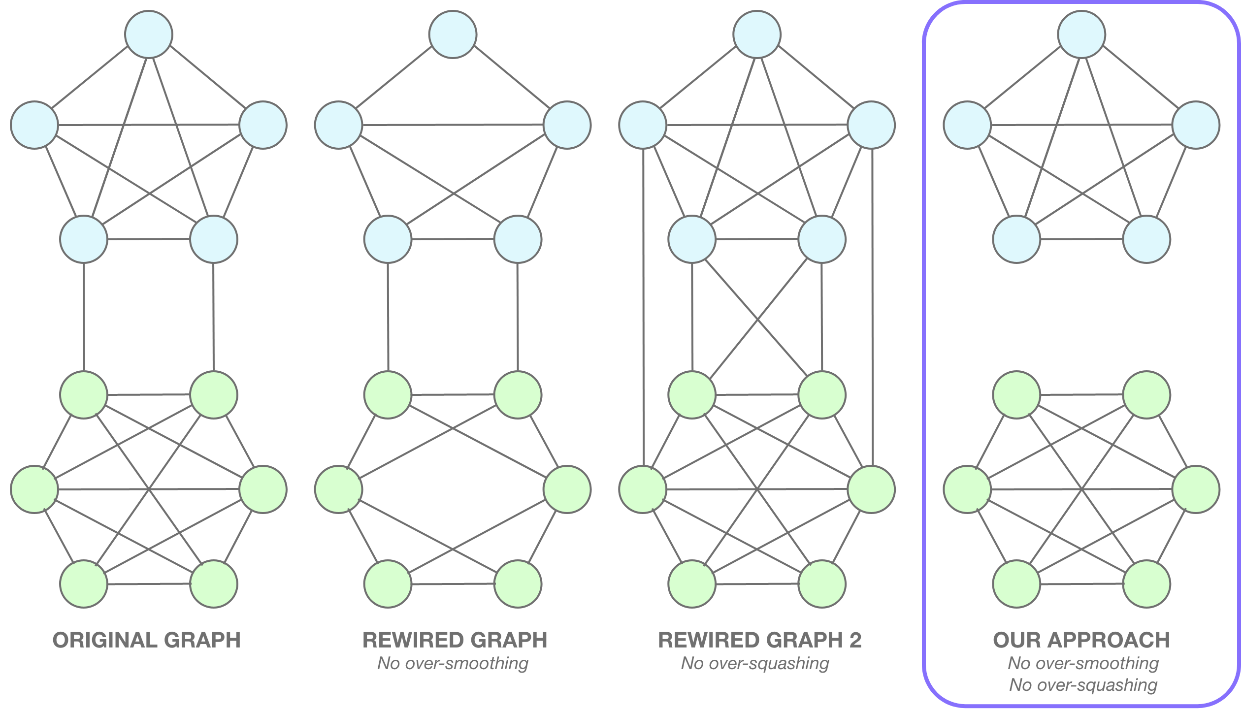
Figure 8: Comparison of graph-rewiring techniques for alleviating over-smoothing and over-squashing. Distinct node colors represent different node classes.

Appendix B Experimental Details: Datasets, Models, and Additional Results

In this work, we evaluated DeltaGNN on 10 distinct datasets. All dataset details are summarized in Table VII. This section describes the models used in this benchmark, as well as the hardware and software configurations employed to run the experiments.

TABLE VI: Dataset details of all datasets.

	# of Graphs	# of Nodes	# of Edges	# of Features	# of Labels	Task Level	Task Type	Training Type	Training Set Size	Validation Set Size	Test Set Size
Planetoid [40]
Cora $\mathcal{H}=0.81$	1	2708	5278	1433	7	Node	Multi-class	Inductive	1208	500	1000
CiteSeer $\mathcal{H}=0.74$	1	3327	4552	3703	6	Node	Multi-class	Inductive	18217	500	1000
PubMed $\mathcal{H}=0.80$	1	19717	44324	500	3	Node	Multi-class	Inductive	1827	500	1000
WebKB [36]
Cornell $\mathcal{H}=0.30$	1	183	295	1703	5	Node	Multi-class	Inductive	87	59	37
Texas $\mathcal{H}=0.09$	1	183	309	1703	5	Node	Multi-class	Inductive	87	59	37
Wisconsin $\mathcal{H}=0.19$	1	251	499	1703	5	Node	Multi-class	Inductive	120	80	51
MedMNIST [9]
Organ-S	1	25221	1276046	784	11	Node	Multi-class	Inductive	13940	2452	8829
Organ-S (dense)	1	25221	2494750	784	11	Node	Multi-class	Inductive	13940	2452	8829
Organ-C	1	23660	1241622	784	11	Node	Multi-class	Inductive	13000	2392	8268
Organ-C (dense)	1	23660	2809204	784	11	Node	Multi-class	Inductive	13000	2392	8268

TABLE VII: Hyperparameter configurations of all datasets.

	# of Layers	Hidden Channels ()thers)	Hidden Channels (GAT)	Hidden Channels (DeltaGNN)	Dropouts	# Removed Edges (Edge-Filter)	# Max Communities	Learning Rate	Optimizer
Planetoid [40]
Cora $\mathcal{H}=0.81$	3	2048	2048	2048	0.5	40/30	20	0.0005	ADAM
CiteSeer $\mathcal{H}=0.74$	3	2048	2048	2048	0.5	40/30	20	0.0005	ADAM
PubMed $\mathcal{H}=0.80$	3	1024	256	1024	0.5	400/200	10	0.0005	ADAM
WebKB [36]
Cornell $\mathcal{H}=0.30$	3	2048	2048	2048	0.5	10/5	20	0.0005	ADAM
Texas $\mathcal{H}=0.09$	3	2048	2048	2048	0.5	10/5	20	0.0005	ADAM
Wisconsin $\mathcal{H}=0.19$	3	2048	2048	2048	0.5	10/5	20	0.0005	ADAM
MedMNIST [9]
Organ-S	3	1024	256	1024	0.5	1000/5000	500	0.0005	ADAM
Organ-S (dense)	3	1024	256	1024	0.5	3000/15000	500	0.0005	ADAM
Organ-C	3	2048	2048	2048	0.5	1000/5000	500	0.0005	ADAM
Organ-C (dense)	3	2048	2048	2048	0.5	3000/15000	500	0.0005	ADAM

TABLE VIII: Comparison of computational resources on datasets of increasing size and density.

Methods	CORA			CiteSeer			PubMed			Organ-S			Organ-S (dense)
	GPU Memory	Preproc. Time	Epoch Time	GPU Memory	Preproc. Time	Epoch Time	GPU Memory	Preproc. Time	Epoch Time	GPU Memory	Preproc. Time	Epoch Time	GPU Memory	Preproc. Time	Epoch Time
GCN [2]	161.81	0.00	0.0014	267.60	0.00	0.0014	779.53	0.00	0.0015	641.31	0.00	0.0016	655.54	0.00	0.0017
GCN + rewiring(DC)	161.81	12.7536	0.0439	267.60	16.0516	0.0549	779.53	123.0887	0.8221	641.31	163.7771	0.8205	655.54	167.4163	0.8388
GCN + rewiring(EC)	161.81	12.7966	0.0440	267.60	16.0762	0.0014	779.53	128.6635	0.8592	641.31	165.3687	0.8284	655.54	168.4002	0.8437
GCN + rewiring(BC)	161.81	36.6763	0.1236	267.60	38.3571	0.1326	OOT	OOT	OOT	OOT	OOT	OOT	OOT	OOT	OOT
GCN + rewiring(CC)	161.81	16.5316	0.0565	267.60	18.8500	0.0642	OOT	OOT	OOT	OOT	OOT	OOT	OOT	OOT	OOT
GCN + rewiring(FC)	161.81	13.2862	0.0457	267.60	16.0841	0.0550	779.53	123.0187	0.8216	641.31	544.1153	2.7222	OOT	OOT	OOT
GCN + rewiring(RC)	161.81	14.2089	0.0488	267.60	16.7696	0.0573	OOT	OOT	OOT	OOT	OOT	OOT	OOT	OOT	OOT
GCN + rewiring(IFS)	161.81	13.5477	0.0465	267.60	17.3902	0.0594	779.53	137.0603	0.9152	641.31	186.4637	0.9339	655.54	188.1741	0.9426
GIN [32]	401.25	0.00	0.0019	507.72	0.00	0.0020	1078.47	0.00	0.0021	867.77	0.00	0.0022	876.75	0.00	0.0024
GIN + rewiring(DC)	401.25	12.7536	0.0444	507.72	16.0516	0.0555	1078.47	123.0887	0.8227	867.77	163.7771	0.8211	876.75	167.4163	0.8395
GIN + rewiring(EC)	401.25	12.7966	0.0445	507.72	16.0762	0.0020	1078.47	128.6635	0.8598	867.77	165.3687	0.8290	876.75	168.4002	0.8444
GIN + rewiring(BC)	401.25	36.6763	0.1241	507.72	38.3571	0.1332	OOT	OOT	OOT	OOT	OOT	OOT	OOT	OOT	OOT
GIN + rewiring(CC)	401.25	16.5316	0.0570	507.72	18.8500	0.0648	OOT	OOT	OOT	OOT	OOT	OOT	OOT	OOT	OOT
GIN + rewiring(FC)	401.25	13.2862	0.0462	507.72	16.0841	0.0556	1078.47	123.0187	0.8222	867.77	544.1153	2.7228	OOT	OOT	OOT
GIN + rewiring(RC)	401.25	14.2089	0.0493	507.72	16.7696	0.0579	OOT	OOT	OOT	OOT	OOT	OOT	OOT	OOT	OOT
GIN + rewiring(IFS)	401.25	13.5477	0.0470	507.72	17.3902	0.0600	1078.47	137.0603	0.9158	867.77	186.4637	0.9345	876.75	188.1741	0.9432
GAT [33]	242.09	0.00	0.0217	336.31	0.00	0.0394	2271.71	0.00	0.0297	2184.78	0.00	0.1042	OOM	OOM	OOM
GAT + rewiring(DC)	242.09	12.7536	0.0642	336.31	16.0516	0.0929	2271.71	123.0887	0.8503	2184.78	163.7771	0.9231	OOM	OOM	OOM
GAT + rewiring(EC)	242.09	12.7966	0.0643	336.31	16.0762	0.0930	2271.71	128.6635	0.8874	2184.78	165.3687	0.9310	OOM	OOM	OOM
GAT + rewiring(BC)	242.09	36.6763	0.1439	336.31	38.3571	0.1706	OOT	OOT	OOT	OOT	OOT	OOT	OOT	OOT	OOT
GAT + rewiring(CC)	242.09	16.5316	0.0768	336.31	18.8500	0.1022	OOT	OOT	OOT	OOT	OOT	OOT	OOT	OOT	OOT
GAT + rewiring(FC)	242.09	13.2862	0.0660	336.31	16.0841	0.0930	2271.71	123.0187	0.8498	2184.78	544.1153	2.8248	OOT	OOT	OOT
GAT + rewiring(RC)	242.09	14.2089	0.0691	336.31	16.7696	0.0953	OOT	OOT	OOT	OOT	OOT	OOT	OOT	OOT	OOT
GAT + rewiring(IFS)	242.09	13.5477	0.0668	336.31	17.3902	0.0974	2271.71	137.0603	0.9434	2184.78	186.4637	1.0365	OOM	OOM	OOM
DeltaGNN - control	539.10	15.4632	0.0540	732.90	18.3549	0.0639	1891.55	142.3362	0.9518	1512.34	213.6147	1.0711	1520.61	245.9796	1.643
DeltaGNN - control + DC	539.10	14.4934	0.0508	732.90	18.3611	0.0639	1891.55	131.6359	0.8805	1512.34	188.6704	0.9463	1520.61	214.6011	1.4338
DeltaGNN - control + EC	539.10	14.7367	0.0516	732.90	17.7273	0.0618	1891.55	131.9083	0.8823	1512.34	197.7688	0.9918	1520.61	226.2949	1.5117
DeltaGNN - control + BC	539.10	38.9384	0.1323	732.90	41.0206	0.1394	OOT	OOT	OOT	OOT	OOT	OOT	OOT	OOT	OOT
DeltaGNN - control + CC	539.10	18.5498	0.0643	732.90	20.8089	0.0720	OOT	OOT	OOT	OOT	OOT	OOT	OOT	OOT	OOT
DeltaGNN - control + FC	539.10	15.1687	0.0531	732.90	18.0004	0.0627	1891.55	135.6264	0.9071	1512.34	555.8835	2.7824	OOT	OOT	OOT
DeltaGNN - control + RC	539.10	15.4131	0.0539	732.90	18.4731	0.0643	OOT	OOT	OOT	OOT	OOT	OOT	OOT	OOT	OOT
DeltaGNN constant	539.14	0.00	0.0372	732.87	0.00	0.0793	1897.26	0.00	0.3860	1540.95	0.00	0.7528	1570.87	0.00	1.2028
DeltaGNN linear	539.14	0.00	0.0372	732.87	0.00	0.0793	1897.26	0.00	0.3860	1540.95	0.00	0.7528	1570.87	0.00	1.2028

Notes: Results are bolded if they are the best result for a certain dataset. OOT indicate an out-of-time error which is generated when the computation of the connectivity measure overruns 30 minutes. OOM indicates an out-of-memory error. The GPU memory is in MB, the epoch and preprocessing times are in seconds.

B-A Evaluation Models

For GCN [2], GIN [32], and GAT [33], we include seven variations that incorporate an edge-rewiring module, which filters edges based on a specific connectivity measure. Specifically, it removes a fixed number of edges from dense areas of the graph to alleviate over-smoothing and removes bottlenecks to prevent over-squashing. We experiment with the following measures: degree centrality (DC), eigenvector centrality (EC), betweenness centrality (BC), closeness centrality (CC), Forman-Ricci curvature (FC), Ollivier-Ricci curvature (RC), and the information flow score (IFS). We also propose two variations of DeltaGNN implementing different functions $K(t,\theta)$; a constant function $K=\theta$, and a linear function:

$$K=\left(\frac{\theta}{T-1}\right)\cdot(t-1)$$

where $T$ denotes the number of layers in the architecture. This last equation describes a line passing through the points $(t=1,K=0)$ and $(t=T,K=\theta)$. Using this function, we ensure that fewer edges are removed in the initial layers and increasingly more are removed in the later ones since $K$ is increasing. This is a desirable property of $K$, as we expect the quality of the IFS to improve with an increasing number of aggregations. Additionally, we include an ablation of DeltaGNN without the IFC mechanism, where edge-filtering is done before homophilic aggregation rather than in parallel (resulting in higher time complexity). We also include seven versions of this model, each implementing different connectivity measures.

The hyperparameters used for each model are detailed in Table VII for reproducibility. To ensure a fair comparison, the number of layers and hidden channels are kept constant across models, with reductions made only in cases of out-of-memory errors. This ensures a balanced comparison of the computational resources used by each method. Fine-tuning has been conducted using a grid-search methodology on the validation set for the following parameters and values: learning rate (0.0001, 0.0005, 0.001, 0.005), edges to remove (values are dataset-specific), maximum number of communities (5, 10, 20, 50, 100, 500), number of layers (3 to 6), and hidden dimensions (100, 256, 512, 1024, 2048).

B-B Experiment Configurations

This section describes the hardware and software configurations used to run the experiments. Our experiments were conducted on a consumer-grade workstation with the following specifications: Intel Core i7-10700 2.90GHz CPU, dual-channel 16GB DDR4 memory clocked at 3200 MHz, and an Nvidia GeForce GTX 1050 Ti GPU with 4GB GDDR5 video memory. The system ran on a Linux-based operating system (Ubuntu 22.04.4 LTS) with NVIDIA driver version 535.183.01 and CUDA toolkit version 12.2. Our implementation uses Python 3.10.12, PyTorch 2.2.0 [47] (with CUDA 11.8), and Torch Geometric 2.5.1 [48]. The results presented are based on 95% confidence intervals over 5 runs, and all datasets were trained inductively. The training pipeline includes an early stopping mechanism with a patience counter to prevent overfitting.

Kevin Mancini received his B.S. degree in Computer Engineering from the Alma Mater Studiorum – University of Bologna, Italy, in 2018, and his M.S. degree in Computer Science from Imperial College London, United Kingdom, in 2024, where he was awarded the ”Splunk Prize for Excellence in MSc Individual Project” for the best individual project in data science and machine learning within the department. He is currently pursuing an M.S. degree in Applied Mathematics and Theoretical Physics at Sapienza University, Rome, Italy. His research focuses on machine learning and deep learning on graphs.

Islem Rekik is the Director of the Brain And SIgnal Research and Analysis (BASIRA) laboratory (http://basira-lab.com/) and an Associate Professor at Imperial College London (Innovation Hub I-X). She is the awardee of two prestigious international research fellowships. In 2019, she was awarded the 3-year prestigious TUBITAK 2232 for Outstanding Experienced Researchers Fellowship and in 2020 she became a Marie Sklodowska-Curie fellow under the European Horizons 2020 program. Together with BASIRA members, she conducted more than 100 cutting-edge research projects cross-pollinating AI and healthcare —with a sharp focus on brain imaging and network neuroscience. She is also a co/chair/organizer of more than 25 international first-class conferences/workshops/competitions (e.g., Affordable AI 2021-22, Predictive AI 2018-2024, Machine Learning in Medical Imaging 2021-24, WILL competition 2021-23). She is a member of the organizing committee of MICCAI 2023 (Vancouver), 2024 (Marrakesh) and South-Korea (2025). She will serve as the General Co-Chair of MICCAI 2026 in Abu Dhabi. In addition to her 160+ high-impact publications, she is a strong advocate of equity, inclusiveness and diversity in AI and research. She is the former president of the Women in MICCAI (WiM), and the co-founder of the international RISE Network to Reinforce Inclusiveness & diverSity and Empower minority researchers in Low-Middle Income Countries (LMIC).

References

- [1] F. Scarselli, M. Gori, A. C. Tsoi, M. Hagenbuchner, and G. Monfardini, “The graph neural network model,” IEEE transactions on neural networks, vol. 20, no. 1, pp. 61–80, 2008.
- [2] T. N. Kipf and M. Welling, “Semi-supervised classification with graph convolutional networks,” Sep 09, 2016. [Online]. Available: https://arxiv.org/abs/1609.02907
- [3] Z. Wu, S. Pan, F. Chen, G. Long, C. Zhang, and P. S. Yu, “A comprehensive survey on graph neural networks,” CoRR, vol. abs/1901.00596, 2019. [Online]. Available: http://arxiv.org/abs/1901.00596
- [4] F. Hu, Y. Zhu, S. Wu, L. Wang, and T. Tan, “Hierarchical graph convolutional networks for semi-supervised node classification,” arXiv preprint arXiv:1902.06667, 2019.
- [5] J. Gilmer, S. S. Schoenholz, P. F. Riley, O. Vinyals, and G. E. Dahl, “Message passing neural networks,” p. 199, 2020.
- [6] M. Zitnik and J. Leskovec, “Predicting multicellular function through multi-layer tissue networks,” CoRR, vol. abs/1707.04638, 2017. [Online]. Available: http://arxiv.org/abs/1707.04638
- [7] D. Ahmedt-Aristizabal, M. A. Armin, S. Denman, C. Fookes, and L. Petersson, “Graph-based deep learning for medical diagnosis and analysis: Past, present and future,” Sensors, vol. 21, no. 14, p. 4758, jul 2021. [Online]. Available: https://doi.org/10.3390%2Fs21144758
- [8] A. Bessadok, M. A. Mahjoub, and I. Rekik, “Graph neural networks in network neuroscience,” 1 2015.
- [9] J. Yang, R. Shi, D. Wei, Z. Liu, L. Zhao, B. Ke, H. Pfister, and B. Ni, “Medmnist v2-a large-scale lightweight benchmark for 2d and 3d biomedical image classification,” Scientific Data, vol. 10, no. 1, p. 41, 2023.
- [10] Q. Li, Z. Han, and X.-M. Wu, “Deeper insights into graph convolutional networks for semi-supervised learning,” in Proceedings of the AAAI conference on artificial intelligence, vol. 32, no. 1, 2018.
- [11] U. Alon and E. Yahav, “On the bottleneck of graph neural networks and its practical implications,” arXiv preprint arXiv:2006.05205, 2020.
- [12] Z. Wu, P. Jain, M. Wright, A. Mirhoseini, J. E. Gonzalez, and I. Stoica, “Representing long-range context for graph neural networks with global attention,” Advances in Neural Information Processing Systems, vol. 34, pp. 13 266–13 279, 2021.
- [13] Z. Fei, J. Guo, H. Gong, L. Ye, E. Attahi, and B. Huang, “A gnn architecture with local and global-attention feature for image classification,” IEEE Access, 2023.
- [14] K. Nguyen, N. M. Hieu, V. D. Nguyen, N. Ho, S. Osher, and T. M. Nguyen, “Revisiting over-smoothing and over-squashing using ollivier-ricci curvature,” in International Conference on Machine Learning. PMLR, 2023, pp. 25 956–25 979.
- [15] F. Barbero, A. Velingker, A. Saberi, M. Bronstein, and F. Di Giovanni, “Locality-aware graph-rewiring in gnns,” arXiv preprint arXiv:2310.01668, 2023.
- [16] T. K. Rusch, M. M. Bronstein, and S. Mishra, “A survey on oversmoothing in graph neural networks,” arXiv preprint arXiv:2303.10993, 2023.
- [17] D. Chen, Y. Lin, W. Li, P. Li, J. Zhou, and X. Sun, “Measuring and relieving the over-smoothing problem for graph neural networks from the topological view,” in Proceedings of the AAAI conference on artificial intelligence, vol. 34, no. 04, 2020, pp. 3438–3445.
- [18] F. Di Giovanni, L. Giusti, F. Barbero, G. Luise, P. Lio, and M. M. Bronstein, “On over-squashing in message passing neural networks: The impact of width, depth, and topology,” in International Conference on Machine Learning. PMLR, 2023, pp. 7865–7885.
- [19] Y. Ollivier, “Ricci curvature of markov chains on metric spaces,” Journal of Functional Analysis, vol. 256, no. 3, pp. 810–864, 2009.
- [20] J. Sia, E. Jonckheere, and P. Bogdan, “Ollivier-ricci curvature-based method to community detection in complex networks,” Scientific reports, vol. 9, no. 1, p. 9800, 2019.
- [21] B. P. Welford, “Note on a method for calculating corrected sums of squares and products,” Technometrics, vol. 4, no. 3, pp. 419–420, 1962.
- [22] S. Yun, M. Jeong, R. Kim, J. Kang, and H. J. Kim, “Graph transformer networks,” Advances in neural information processing systems, vol. 32, 2019.
- [23] V. P. Dwivedi and X. Bresson, “A generalization of transformer networks to graphs,” arXiv preprint arXiv:2012.09699, 2020.
- [24] M. Black, Z. Wan, A. Nayyeri, and Y. Wang, “Understanding oversquashing in gnns through the lens of effective resistance,” in International Conference on Machine Learning. PMLR, 2023, pp. 2528–2547.
- [25] A. Arnaiz-Rodríguez, A. Begga, F. Escolano, and N. Oliver, “Diffwire: Inductive graph rewiring via the lov’asz bound,” arXiv preprint arXiv:2206.07369, 2022.
- [26] K. Karhadkar, P. K. Banerjee, and G. Montúfar, “Fosr: First-order spectral rewiring for addressing oversquashing in gnns,” arXiv preprint arXiv:2210.11790, 2022.
- [27] Y. Yan, M. Hashemi, K. Swersky, Y. Yang, and D. Koutra, “Two sides of the same coin: Heterophily and oversmoothing in graph convolutional neural networks,” in 2022 IEEE International Conference on Data Mining (ICDM). IEEE, 2022, pp. 1287–1292.
- [28] H. Hopf and W. Rinow, “Ueber den begriff der vollständigen differentialgeometrischen fläche,” Commentarii Mathematici Helvetici, vol. 3, no. 1, pp. 209–225, 1931.
- [29] P. Rusnock and A. Kerr-Lawson, “Bolzano and uniform continuity,” Historia Mathematica, vol. 32, no. 3, pp. 303–311, 2005. [Online]. Available: https://www.sciencedirect.com/science/article/pii/S0315086004000849
- [30] K. Mancini and I. Rekik, “Duognn: Topology-aware graph neural network with homophily and heterophily interaction-decoupling,” arXiv preprint arXiv:2409.19616, 2024.
- [31] K. Xu, C. Li, Y. Tian, T. Sonobe, K.-i. Kawarabayashi, and S. Jegelka, “Representation learning on graphs with jumping knowledge networks,” in International conference on machine learning. PMLR, 2018, pp. 5453–5462.
- [32] K. Xu, W. Hu, J. Leskovec, and S. Jegelka, “How powerful are graph neural networks?” arXiv preprint arXiv:1810.00826, 2018.
- [33] P. Velickovic, G. Cucurull, A. Casanova, A. Romero, P. Lio, Y. Bengio et al., “Graph attention networks,” stat, vol. 1050, no. 20, pp. 10–48 550, 2017.
- [34] J. Topping, F. Di Giovanni, B. P. Chamberlain, X. Dong, and M. M. Bronstein, “Understanding over-squashing and bottlenecks on graphs via curvature,” arXiv preprint arXiv:2111.14522, 2021.
- [35] J. Zhu, Y. Yan, L. Zhao, M. Heimann, L. Akoglu, and D. Koutra, “Beyond homophily in graph neural networks: Current limitations and effective designs,” Advances in neural information processing systems, vol. 33, pp. 7793–7804, 2020.
- [36] H. Pei, B. Wei, K. C.-C. Chang, Y. Lei, and B. Yang, “Geom-gcn: Geometric graph convolutional networks,” arXiv preprint arXiv:2002.05287, 2020.
- [37] Y. Shi, Z. Huang, S. Feng, H. Zhong, W. Wang, and Y. Sun, “Masked label prediction: Unified message passing model for semi-supervised classification,” arXiv preprint arXiv:2009.03509, 2020.
- [38] J. Chen, K. Gao, G. Li, and K. He, “Nagphormer: A tokenized graph transformer for node classification in large graphs,” arXiv preprint arXiv:2206.04910, 2022.
- [39] A. K. McCallum, K. Nigam, J. Rennie, and K. Seymore, “Automating the construction of internet portals with machine learning,” Information Retrieval, vol. 3, pp. 127–163, 2000.
- [40] Z. Yang, W. Cohen, and R. Salakhudinov, “Revisiting semi-supervised learning with graph embeddings,” in International conference on machine learning. PMLR, 2016, pp. 40–48.
- [41] C. Adnel and I. Rekik, “Affordable graph neural network framework using topological graph contraction,” in Workshop on Medical Image Learning with Limited and Noisy Data. Springer, 2023, pp. 35–46.
- [42] ——, “Falcon: Feature-label constrained graph net collapse for memory-efficient gnns,” IEEE Transactions on Neural Networks and Learning Systems, 2024.
- [43] Y. LeCun, Y. Bengio, and G. Hinton, “Deep learning,” nature, vol. 521, no. 7553, pp. 436–444, 2015.
- [44] A. A. Efanov, S. A. Ivliev, and A. G. Shagraev, “Welford’s algorithm for weighted statistics,” in 2021 3rd International Youth Conference on Radio Electronics, Electrical and Power Engineering (REEPE). IEEE, 2021, pp. 1–5.
- [45] S. Wandelt, X. Shi, and X. Sun, “Complex network metrics: Can deep learning keep up with tailor-made reference algorithms?” IEEE Access, vol. 8, pp. 68 114–68 123, 2020.
- [46] H. Mao, Z. Chen, W. Jin, H. Han, Y. Ma, T. Zhao, N. Shah, and J. Tang, “Demystifying structural disparity in graph neural networks: Can one size fit all?” Advances in neural information processing systems, vol. 36, 2024.
- [47] A. Paszke, S. Gross, S. Chintala, G. Chanan, E. Yang, Z. DeVito, Z. Lin, A. Desmaison, L. Antiga, and A. Lerer, “Automatic differentiation in pytorch,” 2017.
- [48] M. Fey and J. E. Lenssen, “Fast graph representation learning with pytorch geometric,” arXiv preprint arXiv:1903.02428, 2019.