On the Interaction in Transient Stability of Two-Inverter Power Systems containing GFL inverter Using Manifold Method
Abstract
Many renewable energy resources are integrated into power systems via grid-following (GFL) inverters which rely on a phase-locked loop (PLL) for grid synchronization. During severe grid faults, GFL inverters are vulnerable to transient instability, often leading to disconnection from the grid. Existing studies of this largely focus on the synchronization instability of individual GFL inverters and the interactions between multiple GFL inverters is insufficiently explored. This paper aims to elucidate the interaction mechanisms and define the stability boundaries of systems of two inverters, including GFL, grid-forming (GFM), or grid-supporting (GSP) inverters. First, the generalized large-signal expression for the two-inverter system under various inverter combinations is derived, revealing that no energy function exists for systems containing GFL inverters. This implies that the traditional direct method cannot be applied to such systems. To overcome these challenges, a manifold method is employed to precisely determine the domain of attraction (DOA) of the system, and the transient stability margin is assessed by a new metric termed the critical clearing radius (CCR). A case study of the two-inverter system under various inverter combinations is conducted to explore large-signal interactions across different scenarios. Manifold analysis and simulation results reveal that GSP inverters using PLL for grid synchronization exhibit behavior similar to GFM inverters when the droop coefficients in the terminal voltage control loop (TVC) are sufficiently large. Compared to GFL inverters, GSP inverters incorporating a TVC significantly enhances the transient stability of other inverters. In the STATCOM case, the optimal placement of the STATCOM, realized by GSP or GFM inverters, is identified to be at the midpoint of a transmission line. All findings in this paper are validated through electromagnetic transient (EMT) simulations
Index Terms:
grid-following (GFL) inverter, phase-locked loop (PLL), terminal voltage control, transient stability interactionI Introduction
The grid-following (GFL) inverter, which relies on a phase-locked loop (PLL) for synchronization with the grid, is widely used to interface renewable energy generation with the power grid. However, accidents of PLL losing synchronization when encountering grid fault have been frequently reported in recent years [1, 2]. One major reason is that during a short-circuit fault, the inverter’s terminal voltage is highly sensitive to its output current, which will then cause the PLL to lose synchronization, especially in a weak grid. Additionally, multiple GFL inverters are often interconnected via lines to a common point and then to the grid. The interactions among GFL inverters can affect their synchronization [3] which is different from the single inverter case. Moreover, the interaction between the GFL inverter and other types of inverters, such as grid-forming (GFM) inverters, remains an area that requires further investigation. Since the interaction discussed here refers to the behavior induced by the fault, which is a large-signal perturbation, such interaction is also known as the large-signal interaction, and the system under analysis is nonlinear.
The ability of power systems to re-synchronize after a fault, known as transient stability, has been extensively studied in traditional power systems dominated by synchronous generators (SGs). The direct method avoiding the expensive time-domain integration of the post-fault system dynamics is well-established and has become one of the most widely used approaches [4]. In a nonlinear system, if the initial state of the post-fault system lies inside the domain of attraction (DOA) of this system, it can be concluded, that the system will eventually converge to its post-fault stable equilibrium point (SEP) without the need for the numerical integration. The direct method is to estimate DOA through the level set of energy function (or Lyapunov function). In addition, several methods, including the closest unstable equilibrium point (UEP) method, the controlling UEP method, and the BCU method [4] have been successively proposed to efficiently find this critical level set of the energy function and better estimation of DOA [5]. It should be noted that the construction of analytical energy functions for transient stability analysis is vital in this method. For lossy power systems, [4, 6] proves that the energy functions do not exist for power systems with transfer conductance introduced by the losses. Thanks to the transfer conductance typically being small, even considering the losses, there are still various methods, such as numerical approximations [4], methods based on the extension of the invariant principle [7], and dissipative systems theory [8], which can mitigate this issue in cases of small transfer admittance.
However, in power systems dominated by inverter-based resources (IBRs), the construction of the energy function presents a great challenge, because of the different dynamics between IBR and SG. Furthermore, as demonstrated later in this paper, GFL inverters can introduce cosine interaction terms in the differential equations, similar to the characteristics of transfer conductance. Unfortunately, the cosine interaction terms induced by GFL inverters are much larger than those introduced by transfer conductance, exacerbating this problem. As a result, the global energy function does not exist in power systems containing GFL inverters and there are no effective means to mitigate this issue nowadays, which leads to the failure of the application of the direct method to IBR-dominated systems.
The study in [9] shows that multi-machine systems can be reduced to two clusters, and therefore focusing on two-inverter systems is a reasonable approach to analyzing large-signal interactions. The research on large-signal interaction between two inverters has been covered in [3, 10, 11, 12, 13, 14, 15, 16]. References [3, 16] analyze the stability of multiple GFL inverters only by assessing the existence of SEP to determine transient stability. For two parallel GFL inverters, The oscillation modes when large and small capacity converters are connected in parallel are analyzed in [10], and analyzed by the equal area criteria (EAC). The current injection strategy for the smaller capacity of the inverters is discussed in [11, 15], where the quasi-static analysis is used by judging the existence of SEP. For the parallel GFM and GFL inverters system, the current injection strategy of the GFL inverter is discussed in [12] to achieve more stabilization of GFM inverters. But it is also a quasi-static analysis analysis and the stability of GFL is not taken into account. The paralleled GFM and GFL inverters are also analyzed in [14], where the dynamics of PLL are ignored based on the assumption that the PLL is much faster than the power control loop in GFM inverters. Reference [13] analyzes transient stability based on the voltage of the common connected point and extends EAC to a two-dimensional plane. All the literature above is quasi-static analysis or tries to apply EAC to the two-inverter system, ignoring the dynamic process, instability mode, and characterization of accurate DOA. To address the issues above, this paper presents a geometric method based on the manifold theory, from which the exact DOA of the system can be drawn without conservative or overestimation. The instability mode and bifurcation phenomenon can then be derived from the proposed method. Additionally, a new metric—critical clearing radius (CCR)—is introduced to assess the transient stability margin, and the critical clearing time (CCT) can be derived based on CCR. Compared to the time domain simulation method [17, 18, 19], the computation burden is much less in this method, and post-fault time domain integration is not required.
In summary, the main contributions of this paper are as follows.
-
1)
Derive the generalized large-signal expression for different kinds of inverters, and then indicate that there is no energy function for the system containing GFL Inverters;
-
2)
In order to tackle the analysis difficulty above, a geometric method based on the manifold theory is proposed, and the metric CCR is introduced to assess the transient stability.
-
3)
Large-signal interactions in various two-inverter systems are studied, and various new oscillation patterns are identified;
-
4)
The similarities between grid-supporting (GSP) inverters, which incorporate terminal voltage control (TVC) into GFL inverters, and GFM inverters are investigated, revealing the role of TVC in enhancing system dynamics.
The rest of the article is organized as follows. Section II describes the modeling of systems with combinations of different types of inverters and derives the generalized large-signal expression. The manifold method and the new metric CCR are illustrated in Section III. The case study and EMT simulation of the selected system are discussed in Section IV. Finally, Section V concludes this article.
II The Modelling of The System Containing GFL Inverters
II-A Large-signal Modelling of Different Types of Inverters.
II-A1 GFM inverter
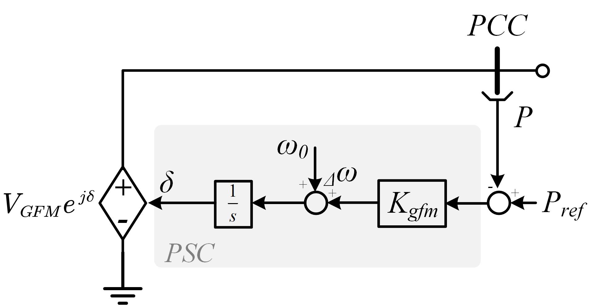
In general, the inner voltage control loop in the GFM inverter is typically ignored since it is much faster than the outer control loop such as the power synchronous controller (PSC), and thus the GFM inverters are regarded as an ideal controlled voltage source when analyzing its large-signal dynamics [2, 12]. The large-signal modeling of GFM inverters is illustrated in Figure 1(a), and the dynamics are as follows, irrespective of the connected grid:
| (1) |
where the angle change of the inverter is denoted as , and is the droop coefficient in the GFM inverter, and and represent the real output power of the GFM inverter and the power reference of the GFM inverter.
II-A2 GFL inverter
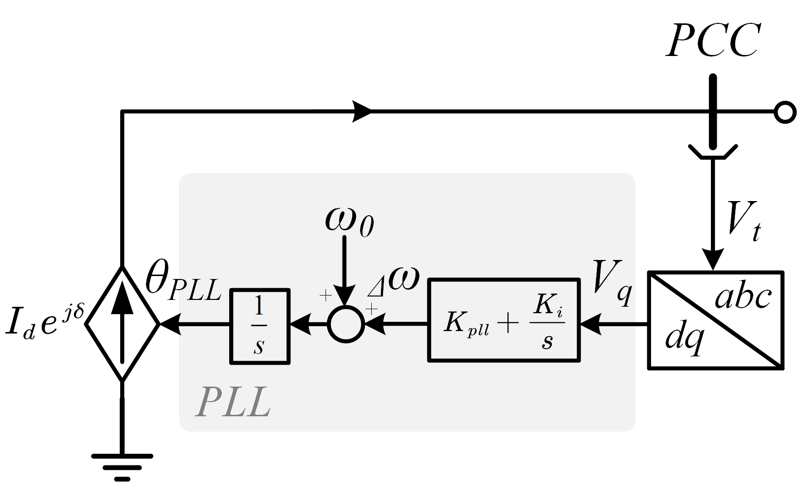
The large-signal modeling of a typical GFL inverter is illustrated in Figure 1(b), where the GFL inverter is typically regarded as a controlled current source, since the inner current control loop is much faster than PLL [15, 19]. The current reference of the GFL inverter is fixed, and only PLL is taken into account in the large-signal analysis. The nonlinear dynamics can be expressed as
| (2) |
The research in [20, 21] indicates that the small integral term and large proportional term are beneficial to transient stability. Hence, the PI controller is usually designed to be over-damped, that is , where the existence of a small is only used to eliminate a steady-state offset. As a result, the proportional term is much faster than the integral term in the PI controller of the PLL.
II-A3 GSP inverter
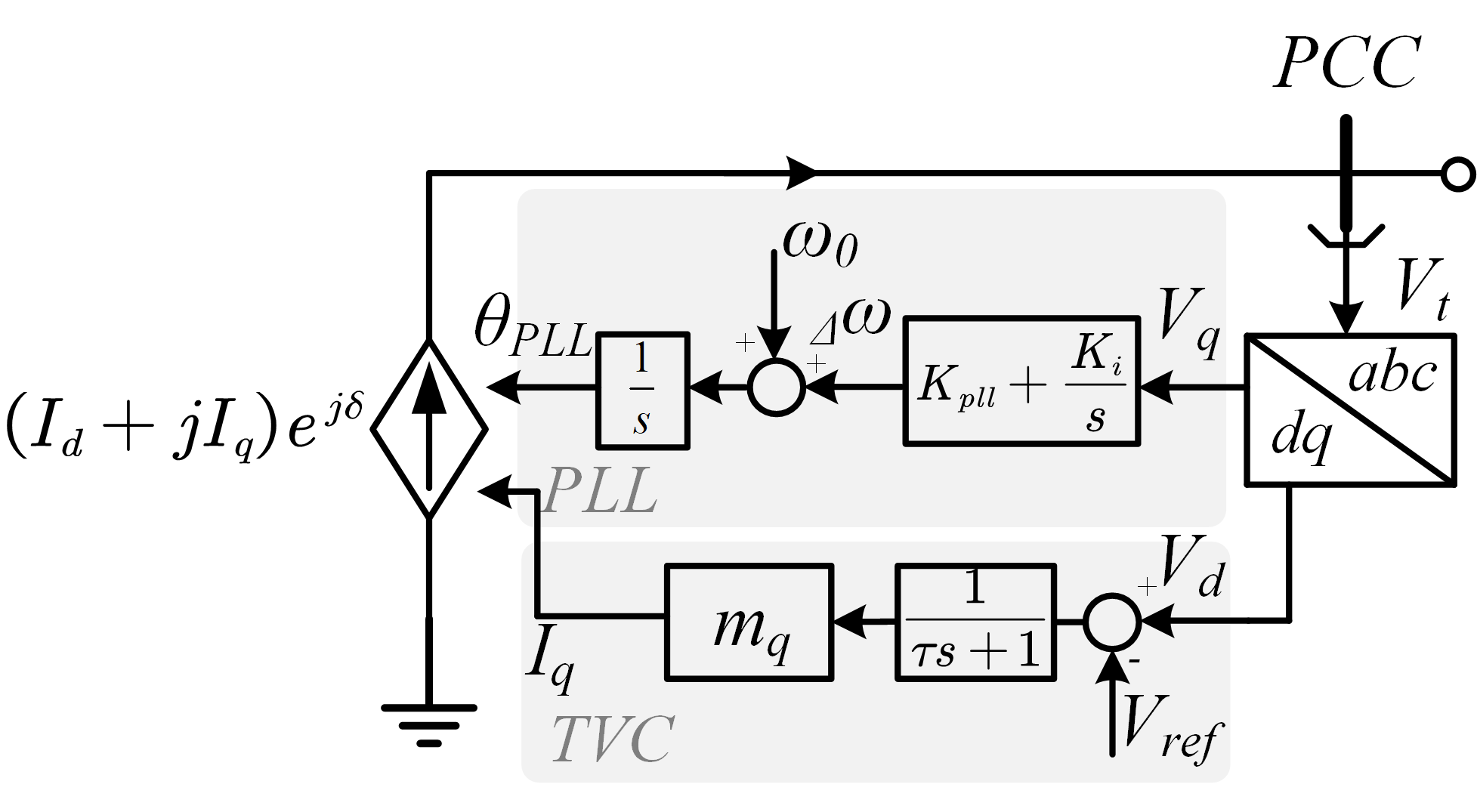
In order to realize voltage support, in some cases, the terminal voltage control (TVC) loop is added to the GFL inverter as illustrated in Figure 1(c), which is a widely adopted approach. In this paper, such GFL inverters equipped with TVC are designated as grid-supporting (GSP) inverters. In TVC, droop control is applied to control the injection of the reactive current according to grid code [22, 23]. Since the TVC is typically much faster than the PLL [24], thus the voltage control dynamics can be simplified as the algebraic equation [25]. The modeling is as follows regardless of the connected grid:
| (3a) | ||||
| (3b) | ||||
where represents the -axis value of the terminal voltage, and is defined as the -axis current namely the negative reactive current, and is the droop coefficient in TVC.
It can be seen that the dynamics of the PLL in both GFL and GSP are of second order. In order to apply manifold theory and accurately depict the DOA of the two-inverter system in a two-dimensional phase plane, it is necessary to reduce the order of the model of PLL. Thanks to being much larger than , the integral term can be ignored according to singular perturbation theory [25]. Consequently, the dynamics of the PLL in GFL and GSP inverters can be modeled as
| (4) |
In the simulation part, the results will indicate that the integral term has minimal impact on the PLL dynamics and almost no influence on the DOA.
| IBR1 | IBR2 | ||||||||||
| GFM | GFM | 0 | 0 | ||||||||
| GFM | GFL | 0 | 0 | ||||||||
| GFM | GSP | 0 | 0 | ||||||||
| GFL | GFL | 0 | 0 | ||||||||
| GFL | GSP | 0 | 0 |
II-B Modelling of the Whole Two-IBR System
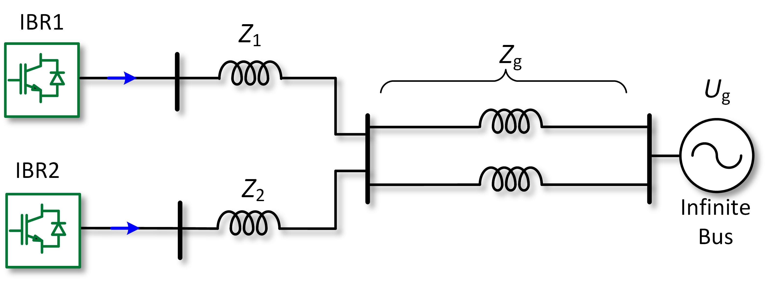
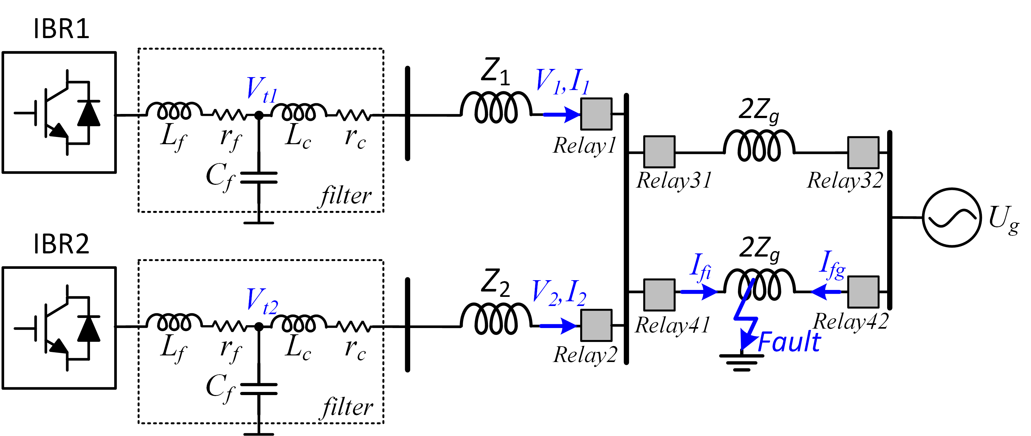
To assess how one inverter has an impact on the stability of another, the test system shown in Figure 2 was established in which two IBRs can be configured as GFL, GFM, or GSP inverters. These inverters are connected via transmission lines to a common point, which in turn is connected to an infinite bus.
II-B1 Both IBRs are GFM inverters
When both the two IBRs in Figure 2 are GFM inverters, the nonlinear differential equations describing the system are as follows:
| (5) |
The expression of , , are defined in Appendix A-A. In (5), , , and , represent the power angles, and the power references of the two GFM inverters respectively. and are the voltages of two GFM inverters.
II-B2 Both IBRs are GFL inverters
When both the two IBRs in Figure 2 are GFL inverters, the nonlinear differential equations describing the system are as follows:
| (6) |
The expression of , are defined in Appendix A-A. In (6), , , and , represent the angles of PLL, and the current references on -axis of the two GFL inverters respectively.
II-B3 Combination of IBR1 as a GFL inverter and IBR2 as a GFM inverter
II-B4 Combination of IBR1 as a GFL inverter and IBR2 as a GSP inverter
When IBR1 is the GFL inverter and IBR2 is the GSP inverter in Figure 2, the nonlinear differential equations describing the system can be expressed jointly by (6) and (3b), which can be simplified to (8). The detailed simplification process and the terms , are demonstrated in Appendix A-B.
| (8) |
In (8), the definition of represents the voltage control error. The represents dynamics of the difference between the angle of PLL2 and its steady state.
When is large enough, which means that the dynamic of PLL2 is much faster than PLL1, the perturbed term can be regarded as zero. Also, when the droop coefficient is large enough, indicating more effective voltage control with smaller error, the term is approximately 1. Under this case (, ), the sets of Equations (7) and (8) are identical, and they share the same form as follows:
| (9) |
where represents a constant.
II-B5 Combination of IBR1 as a GSP inverter and IBR2 as a GFM inverter
When IBR1 is the GFL inverter with TVC and IBR2 is the GFM inverter in Figure 2, the nonlinear differential equations describing the system can be expressed jointly by (7) and (3b), which can be simplified to (10). The detailed simplification process and the terms , are demonstrated in Appendix A-C.
| (10) |
In (10), the definition of represents the voltage control error. The represents dynamics of the difference between the angle of PLL1 and its steady state.
When is large enough, which means that the dynamic of PLL1 is much faster than PLL2, the perturbed term can be regarded as zero. Also, when the droop coefficient is large enough, indicating more effective voltage control with smaller error, the term is approximately 1. Under this case (, ), the sets of Equations (10) and (5) are identical, and they share the same form as follows:
| (11) |
where , , , , , represent constants.
II-C Generalized expression and non-existence of energy function
The generalized differential equations of two-IBR systems can be expressed in (12).
| (12) |
The coefficients in (12) are shown in Table I. When the system comprises only SG and GFM, the differential equations describing the system dynamics contain only sine terms, such as . The system, in this case, has an energy function as illustrated in Appendix B. In Table I, when the GFL inverter exists in the system, cosine term exists in the nonlinear differential equations. The existence of voltage control in the GFL inverter can transform cosine term to sine term .
In traditional power systems, cosine terms are typically introduced by the presence of transfer conductance. In the literature, Chiang [6] demonstrated that if the dynamics of a system, as described by (12), include cosine terms, no energy function exists. Similarly, if the system contains GFL inverters, as described by (12), an energy function also cannot be established. Furthermore, the coefficient of the cosine term, influenced by the magnitude of the current reference , has a more pronounced effect than that of the transfer conductance. Consequently, the direct method is inapplicable in systems with GFL inverters, necessitating the development of a new method for transient stability assessment.
III Transient Stability Assessment Based on Manifold Method and CCR
III-A Real DOA derivation based on manifold theory
The manifold theory regarding the Domain of Attraction (DOA) as proposed by Chiang [4, 5] is articulated as follows. Consider a nonlinear autonomous dynamical system described by:
| (13) |
If (13) meets the following criteria: 1) All the equilibrium points (EPs) on the stability boundary are hyperbolic; 2) The stable and unstable manifolds of EP on the stability boundary satisfy the transversality condition; 3) Every trajectory on the stability boundary approaches one of the critical elements as , and these assumptions are readily met in two-inverter systems. Then the stability boundary of a SEP, denoted ,comprises the union of the stable manifolds of UEPs, , and the stable manifolds of closed orbits, , which can be expressed as
| (14) |
For a two-dimensional system analyzed in this paper, the UEP on the stability boundary is either a type-I UEP or a type-II UEP, and the stable manifold of a type-I UEP is one dimension (curve). The real DOA can be drawn by the following steps:
-
1)
Find the Jacobian at each unstable equilibrium point (UEP), .
-
2)
Find the stable eigenvectors of the Jacobian and the normalized vectors in the subspace spanned by stable eigenvectors, .
-
3)
Find the intersection of each of these normalized vectors with the boundary of an -ball of the equilibrium point (the intersection points are ).
-
4)
Integrate backward the vector field (i.e. in reverse time) from each of these intersection points up.
-
5)
The real DOA can be derived.
III-B Proposed transient stability metrics - CCR
In order to assess the transient stability margin, a new metric - critical clearing radius (CCR) is proposed, which intuitively measures the distance from the post-fault SEP to the stability boundary. The CCR is defined as the shortest distance between the SEP and the real DOA, which is , as shown in Figure 3.
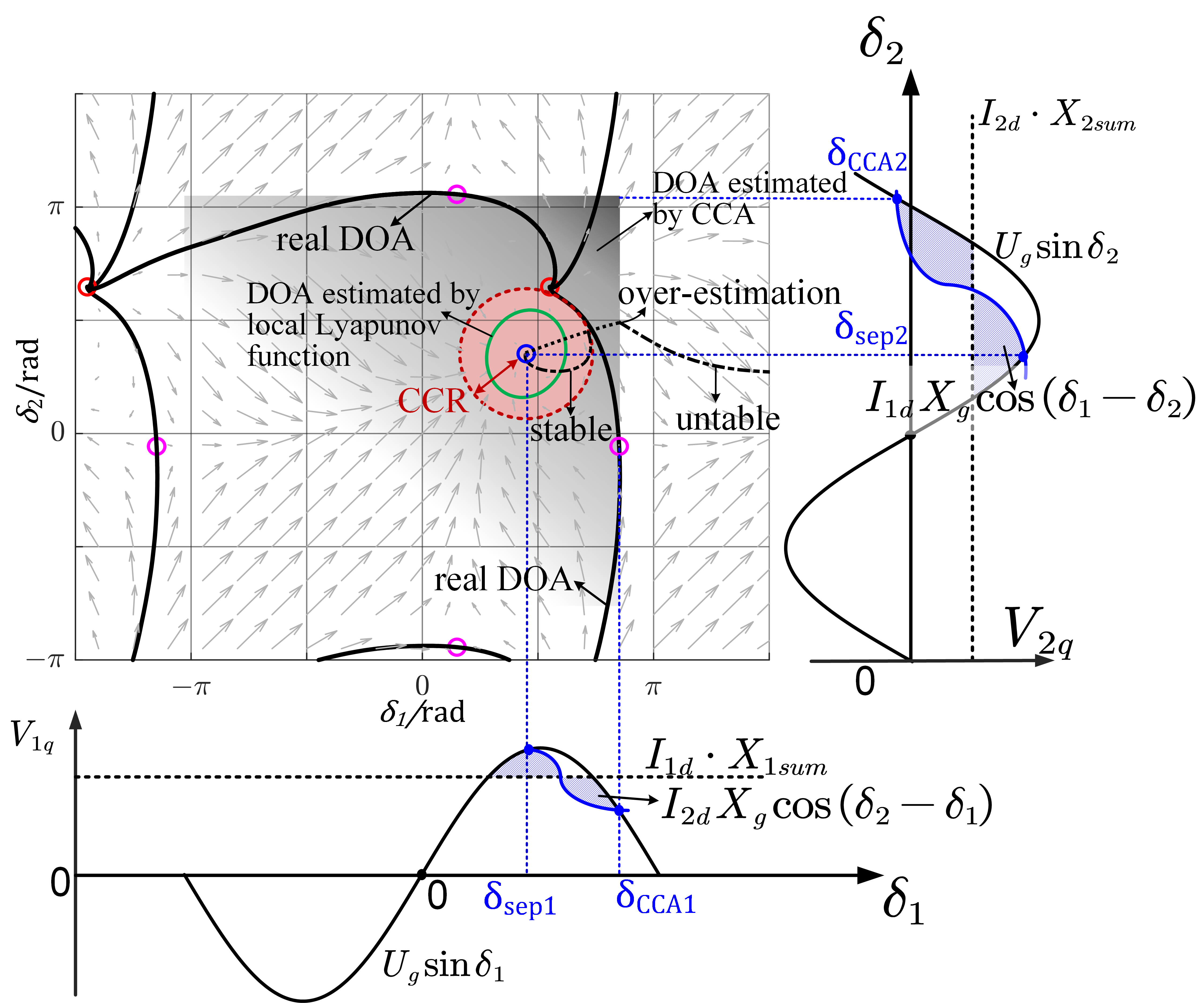
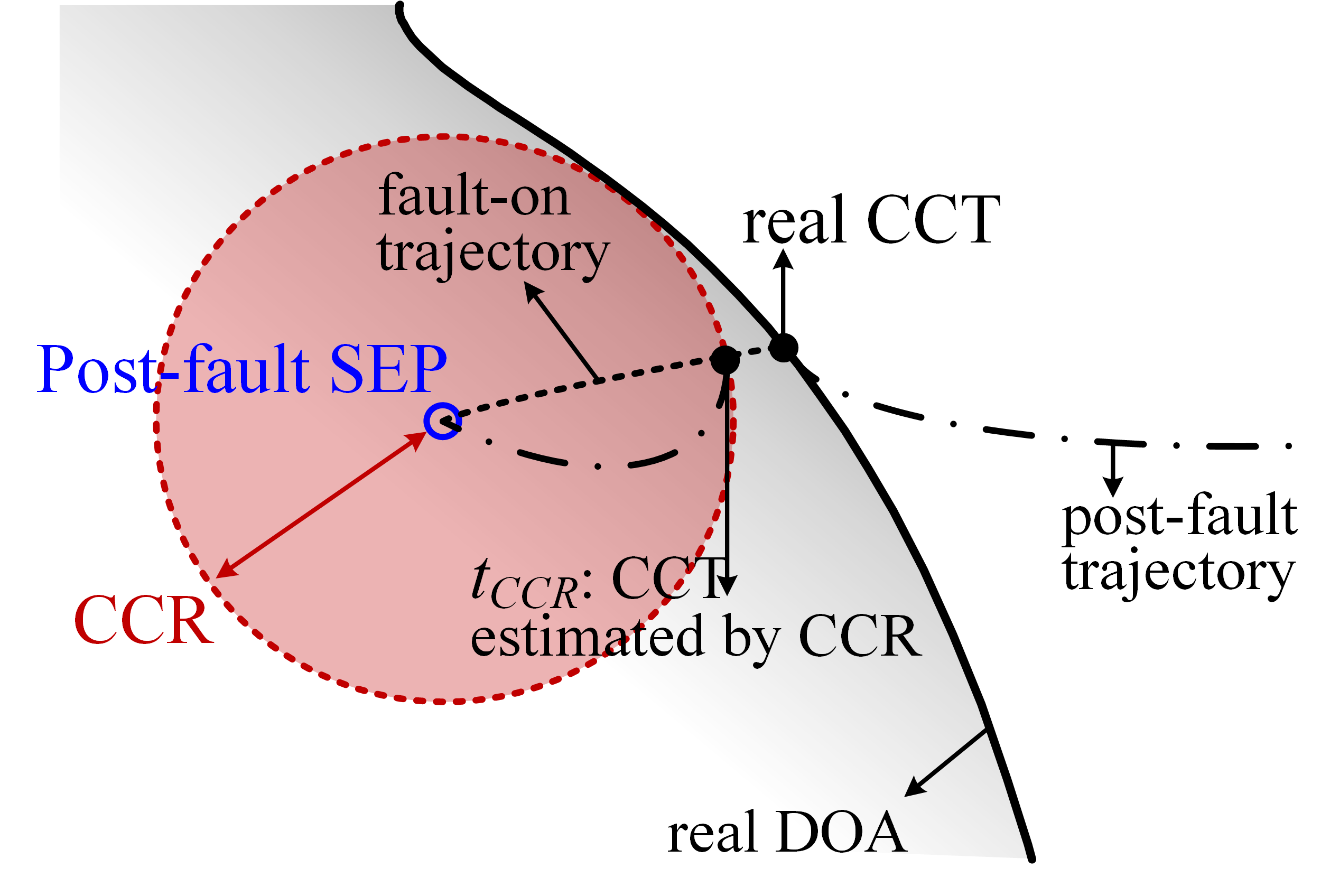
Figure 3 compares the CCR with other transient stability methods applied in the two GFL inverters system. The critical clearing angle is the projection of real DOA to , coordinates, denoted by . This can also be represented by the intersection between the sine function and the blue solid curve in Figure 3. Due to the existence of interaction terms (e.g. ), there is the difference between the blue solid curve and the dotted lines (e.g. ), as shown in the blue shaded area between two curves. Reference [12, 11] accepted this method, taking the CCA of the large-capacity GFL as the transient stability index of the system. However, the transient stability derived by one-dimensional CCA neglects the interaction and causes an overestimation of the DOA, as shown in the grey rectangle area in Figure 3. In particular, if two inverters are connected both to the infinite bus, then the DOA is square, which means the boundary of has no relationships with , and vice versa. The two inverters are decoupled from each other, and the .
The local Lyapunov function to estimate the DOA is also plotted as the green curve in Figure 3, which is an approach to address the situation where the global energy function does not exist. The local Lyapunov function is derived from the Lyapunov equation at SEP. It can be seen that the local Lyapunov method can usually cause under-estimation for the DOA.
The calculation of CCR is straightforward, which requires recording the shortest distance to the postfault SEP When doing the backward integration to find the true DOA. it is also convenient to generalize to higher dimensional situations. Furthermore, CCT can be estimated based on CCR. The specific steps are: 1) integrate the fault-on trajectory ; 2) At the time , if is outside of the circle of CCR, but is inside of the circle of CCR. is the Integration step; 3) The is the CCT estimated by CCR. Since the CCR is inside the real DOA, the conservativeness of estimated CCT by CCR, , can be guaranteed. The relationships between proposed CCR, and real DOA and CCT are illustrated in Figure 4.
To sum up, the manifold method completely describes the whole dynamic behavior in the phase plane, and the CCR proposed based on this method is an extension of CCA in high-dimensional space, which can describe the relative transient stability of systems being considered.
When fault clearing occurs at a time that gives a position outside the stability boundary around the SEP, the trajectory will not converge to this SEP. It should be noted that even though sometimes the trajectory may converge to a different SEP that is one period away from the original SEP, this is considered unstable in engineering terms [26, 27]. This case is analogous to the pole slipping of a synchronous generator and will cause the over-voltage of GFL inverters and impact the impedance measurement in the distance protection and thus jeopardize the system operation [28].
IV Case Study Based on Proposed Manifold Method
The case study and simulations are carried out in this part, and the tested system has been illustrated in Figure 5. The time-domain EMT simulation is done by MATLAB\Simulink.
IV-A Combination of both IBR1 and IBR2 as GFL inverters
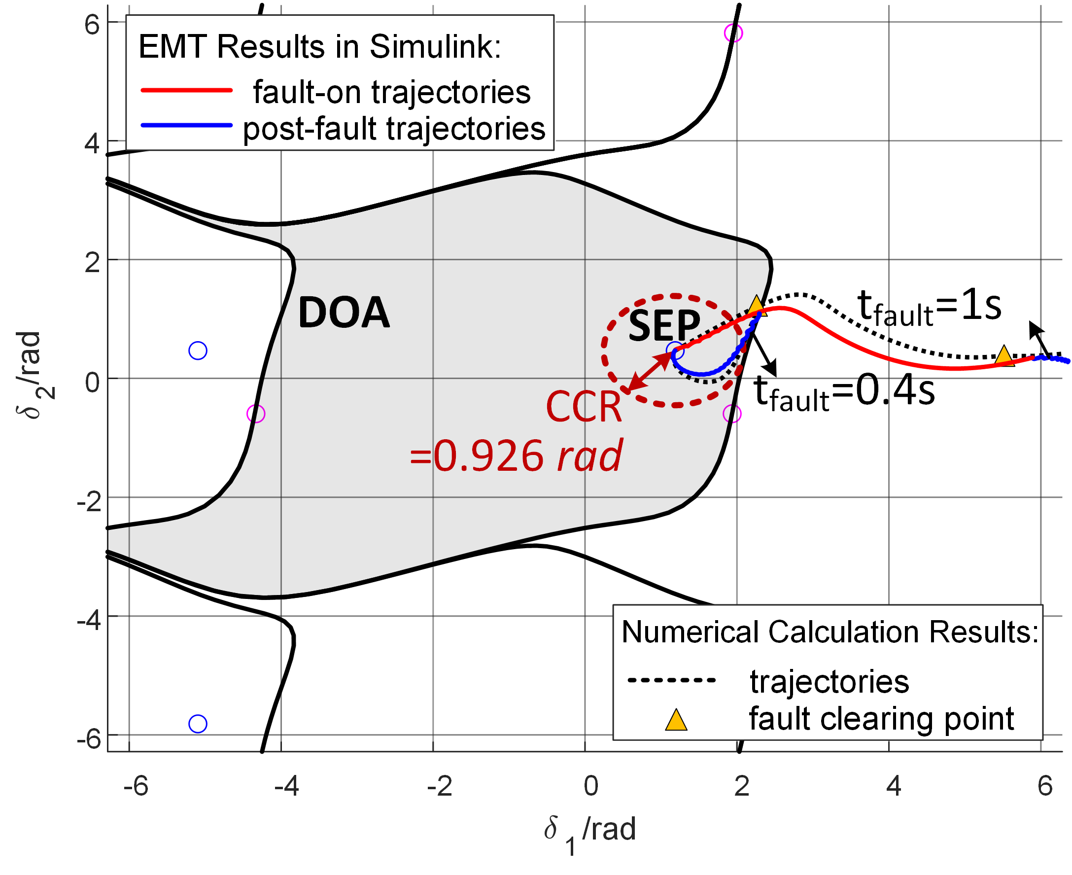
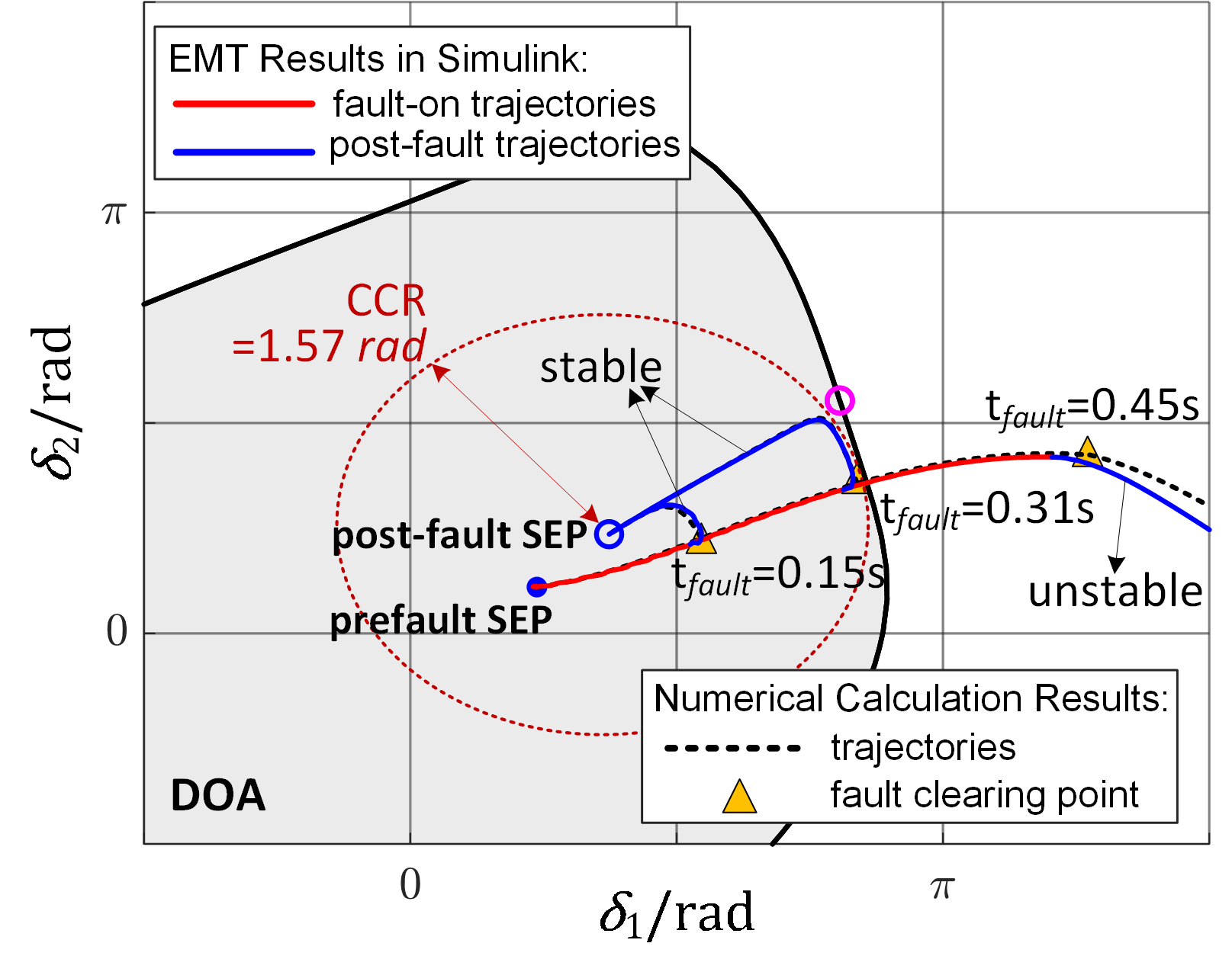
In this section, the accuracy of the reduced-order PLL model, the proposed geometric method, and CCR and the CCT estimated by CCR, denoted by , are verified through EMT simulations. Both IBR1 and IBR2 are configured as grid-following (GFL) inverters in Figure 5. The PLLs of two inverters are designed to be over-damped, with the integral gain set to the one-tenth of the proportional gain . Under this configuration, the contribution of the integral term is negligible, and the proportional term primarily governs the dynamic behavior. The line impedance is set to either or , and at time 0.5s, a fault is introduced in the middle of transmission line . For , the CCR is calculated as 0.90 rad, and the CCT estimated by CCR, , is 0.212s; while when the CCR is calculated and decreased to 0.53 rad, and the CCT estimated by CCR, , is 0.131s. In EMT simulation the fault clearing times are set as 0.212s and 0.25s when , and 0.131s and 0.212s when . After fault clearance, the line impedance is doubled in the post-fault system. Detailed system parameters are presented in Table A1 (see Appendix B).
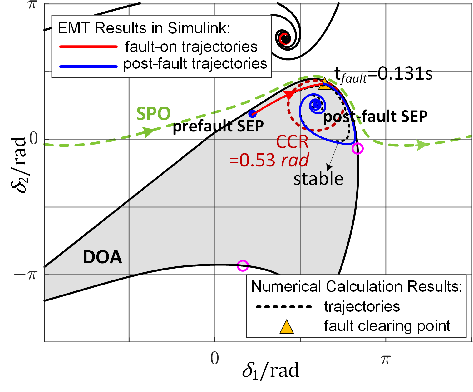
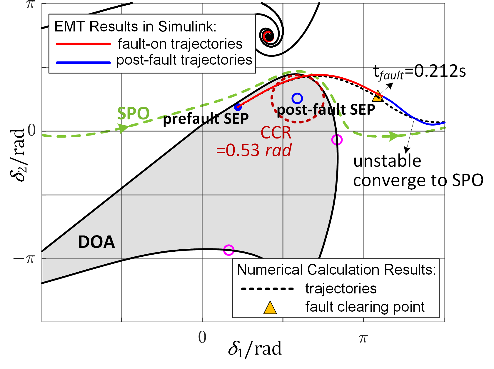
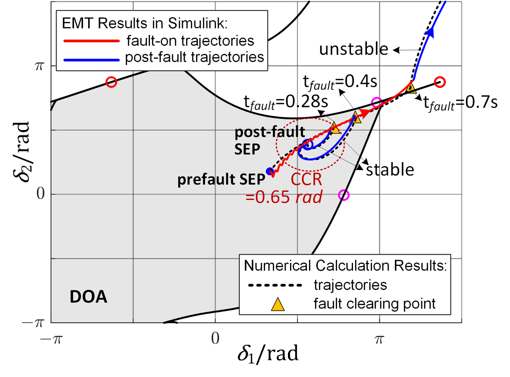
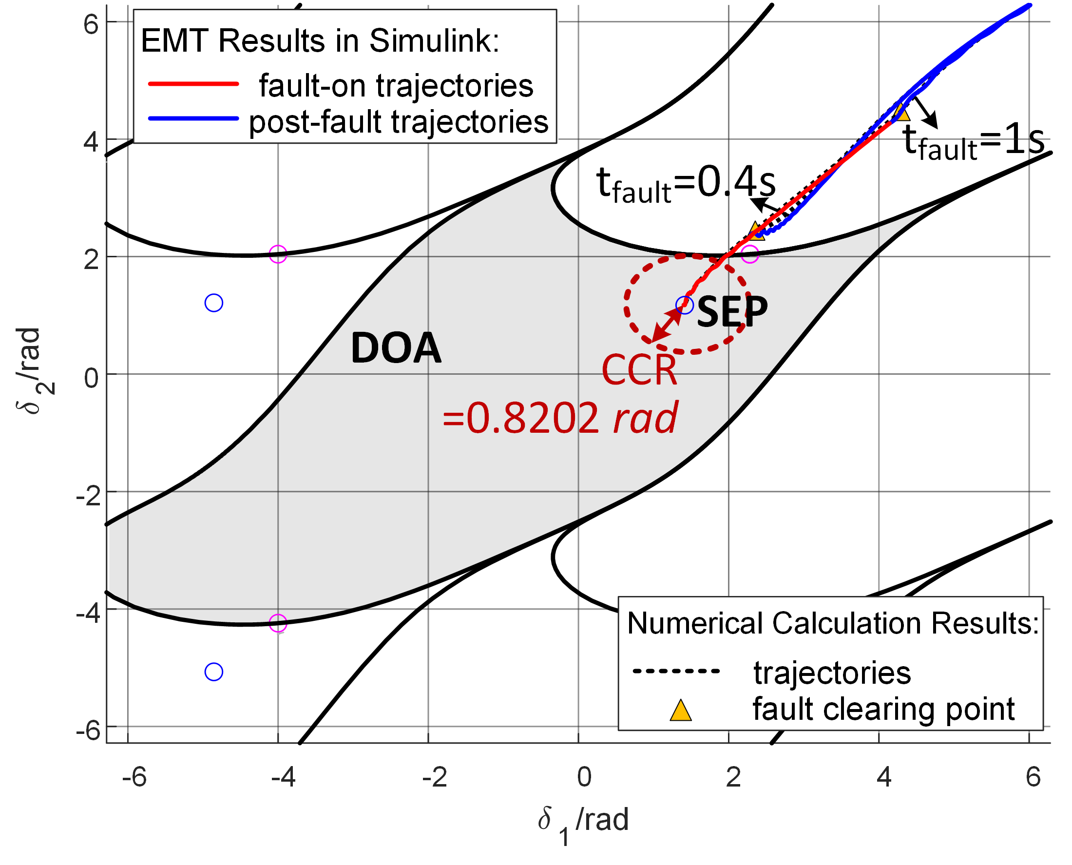
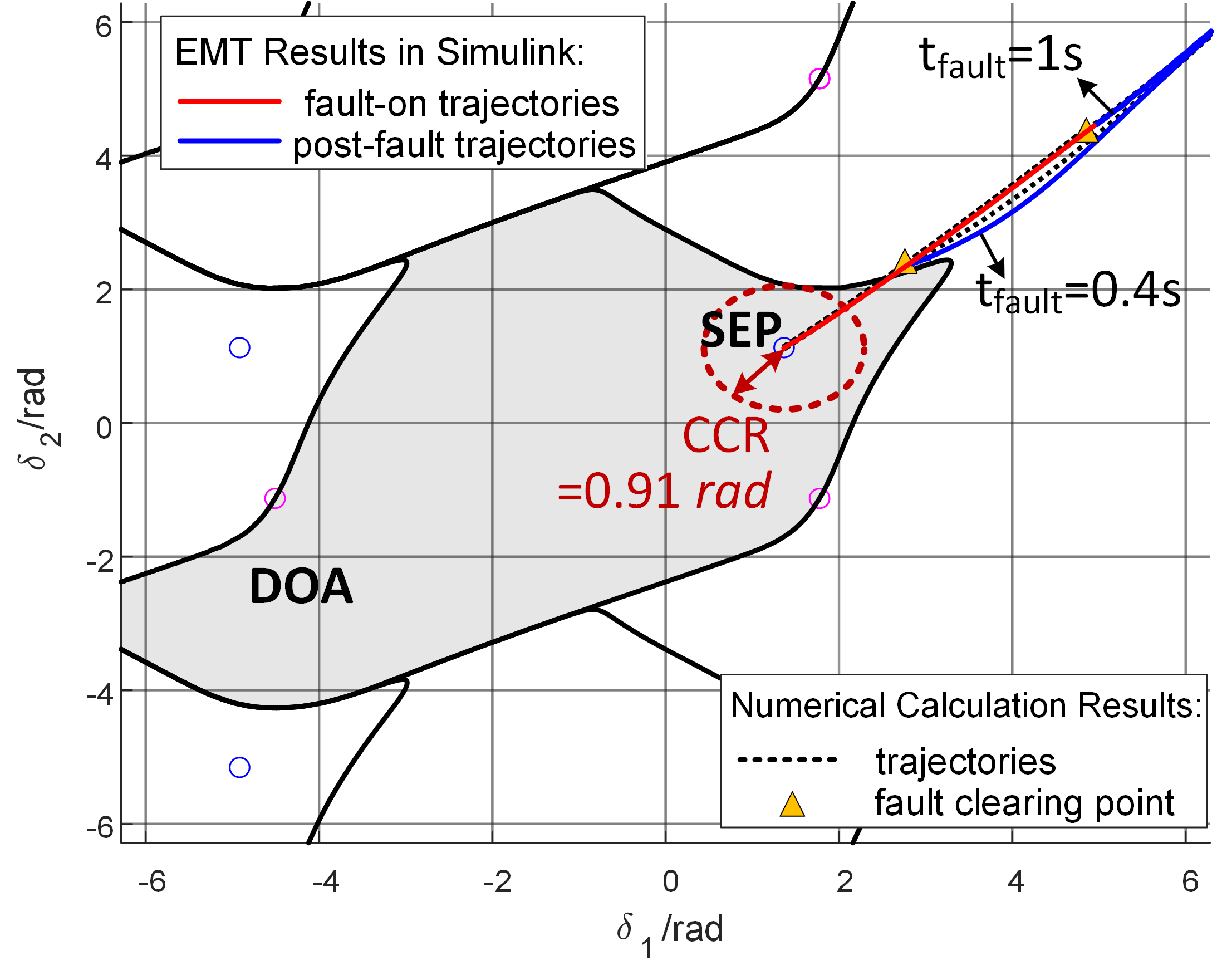
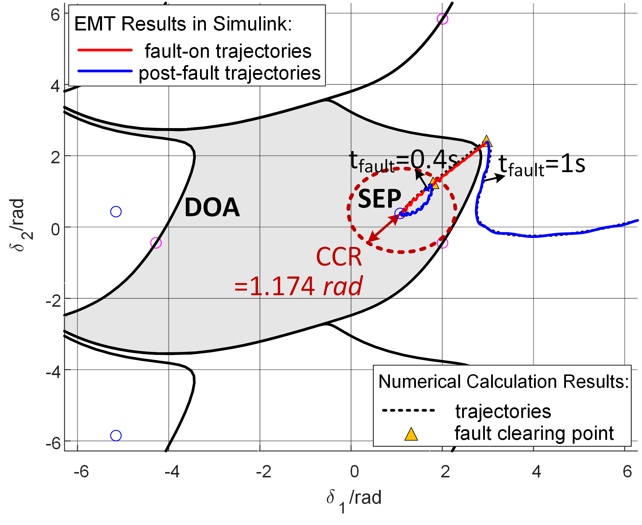
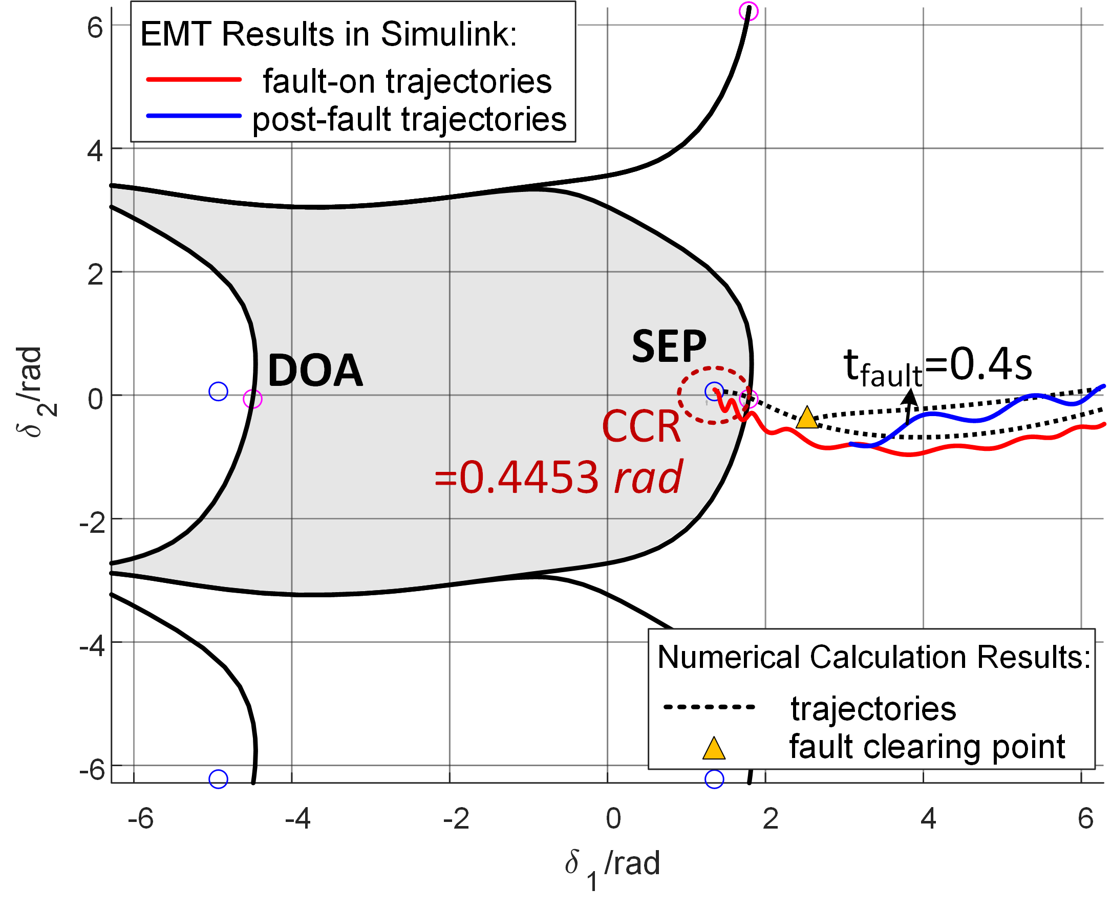
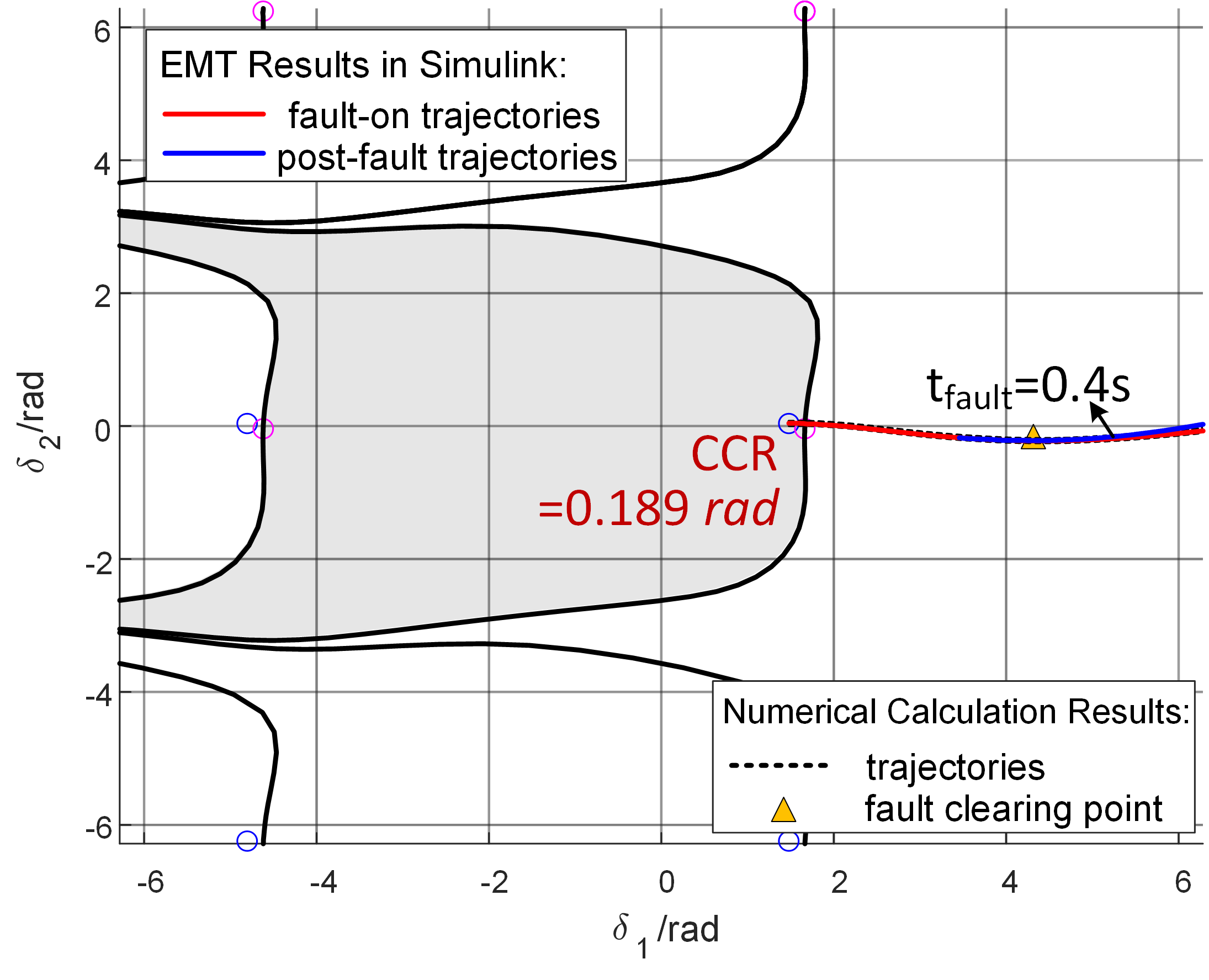
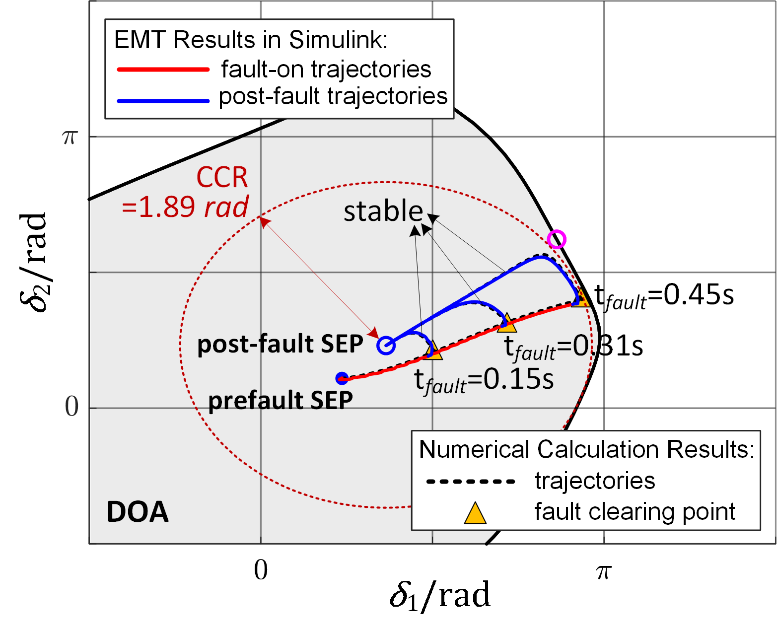
According to the manifold method, the DOA, represented by the grey shaded area, and CCR, indicated by the red dashed circle, can be drawn in Figure 6(a)(b) and (c)(d) when , and respectively. When as shown in Figure 6(c)(d), a stable periodical orbit (SPO) emerges in the post-fault system, depicted as a green dashed curve in the phase plane. This indicates a new instability mode in this case. When the trajectory lies outside the DOA, it converges to this SPO, leading to divergence of and sustained oscillations in .
Figure 6 compares the phase portraits derived from numerical calculations based on the theoretical model and EMT simulations. The black dashed lines represent the trajectories of the two PLLs as determined by numerical calculations, with yellow triangle markers indicating the fault-clearing points. The red solid lines show the fault-on trajectories from EMT simulations, while the blue solid lines illustrate the post-fault trajectories for different fault-clearing times. Overall, the EMT simulation results align well with the theoretical model. The observed differences can be attributed to factors not included in the theoretical model, such as the inner current loop dynamics, the integral terms in the PLL, and the influence of the actual circuit implementation.
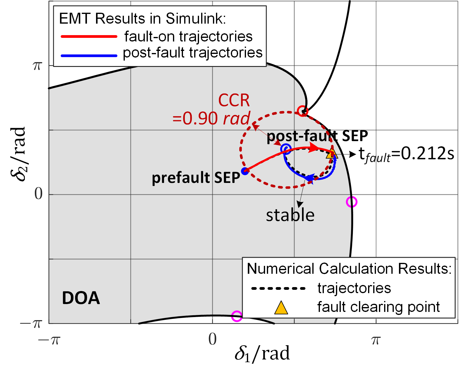
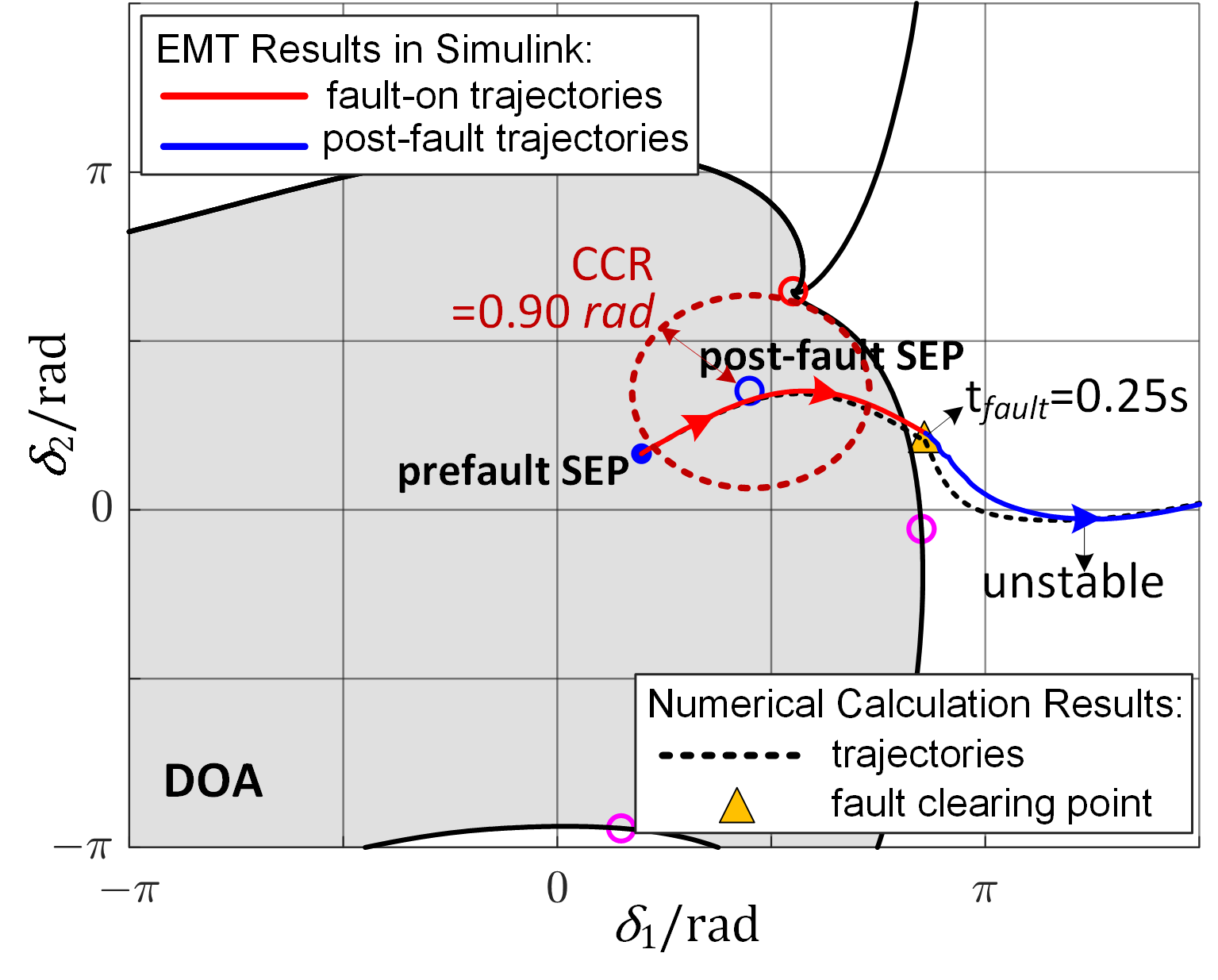
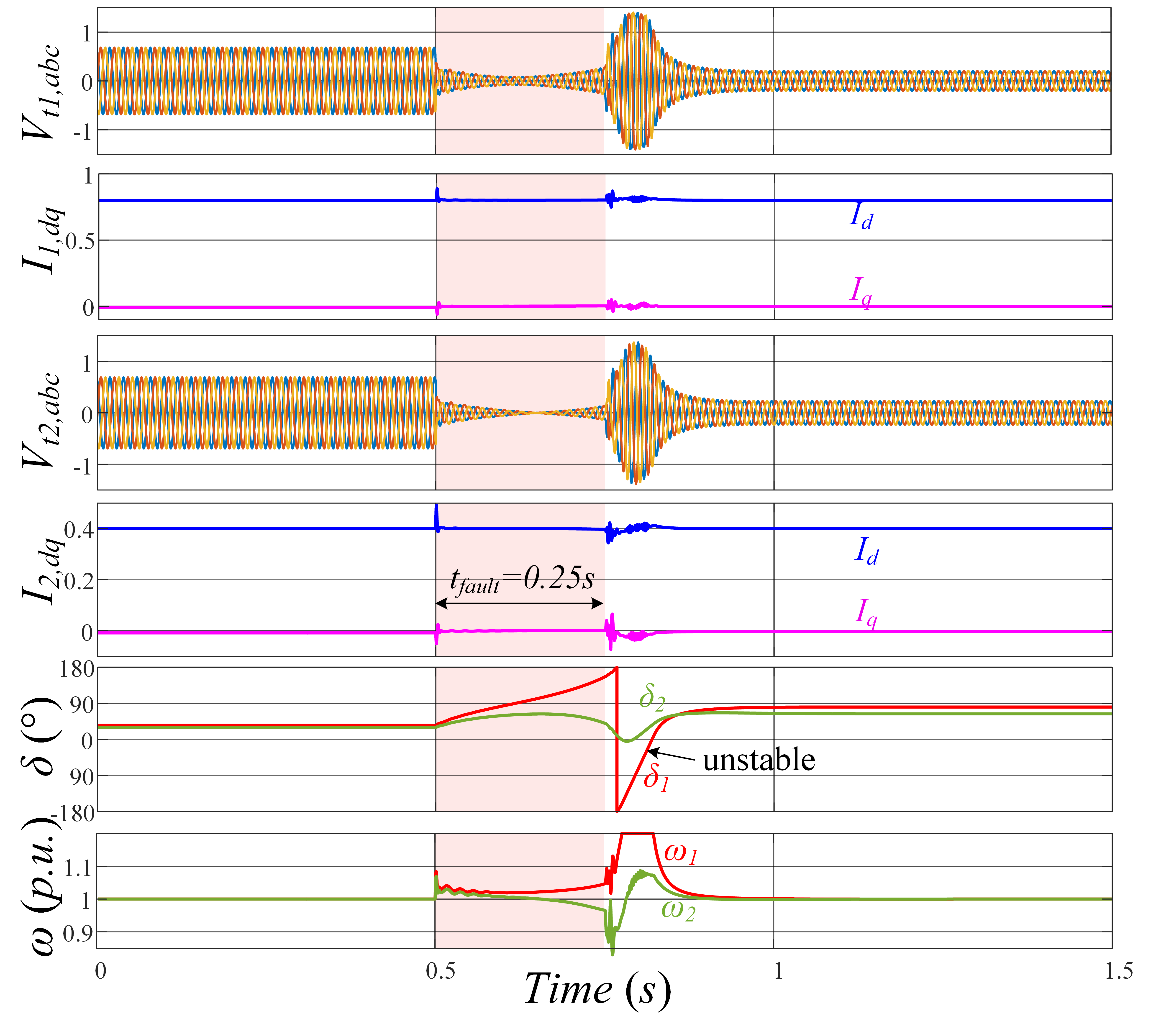
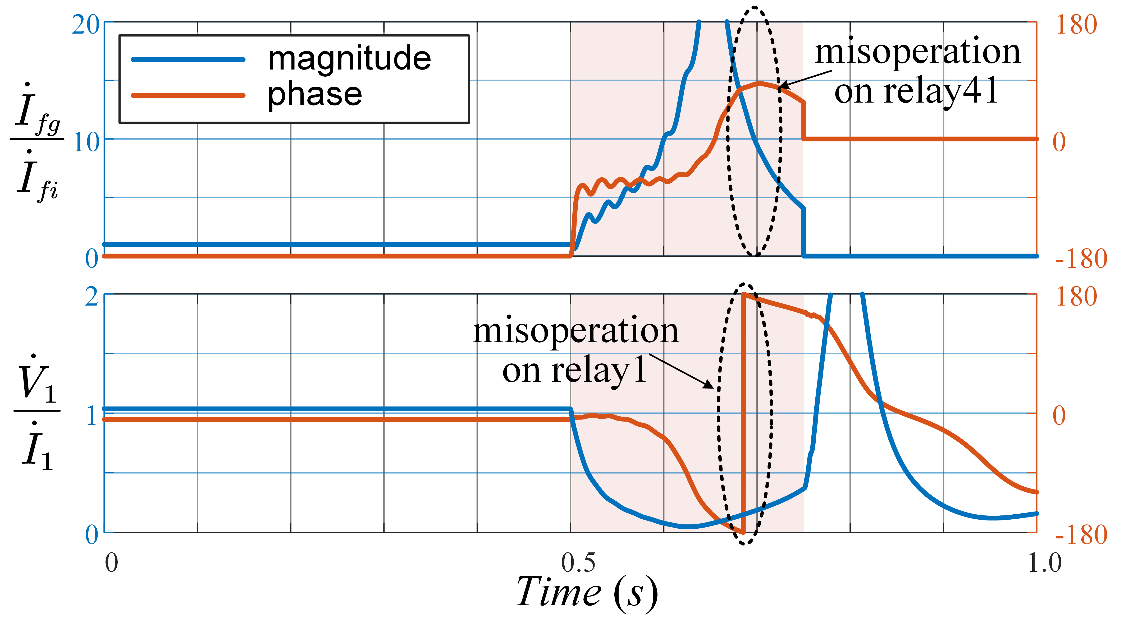
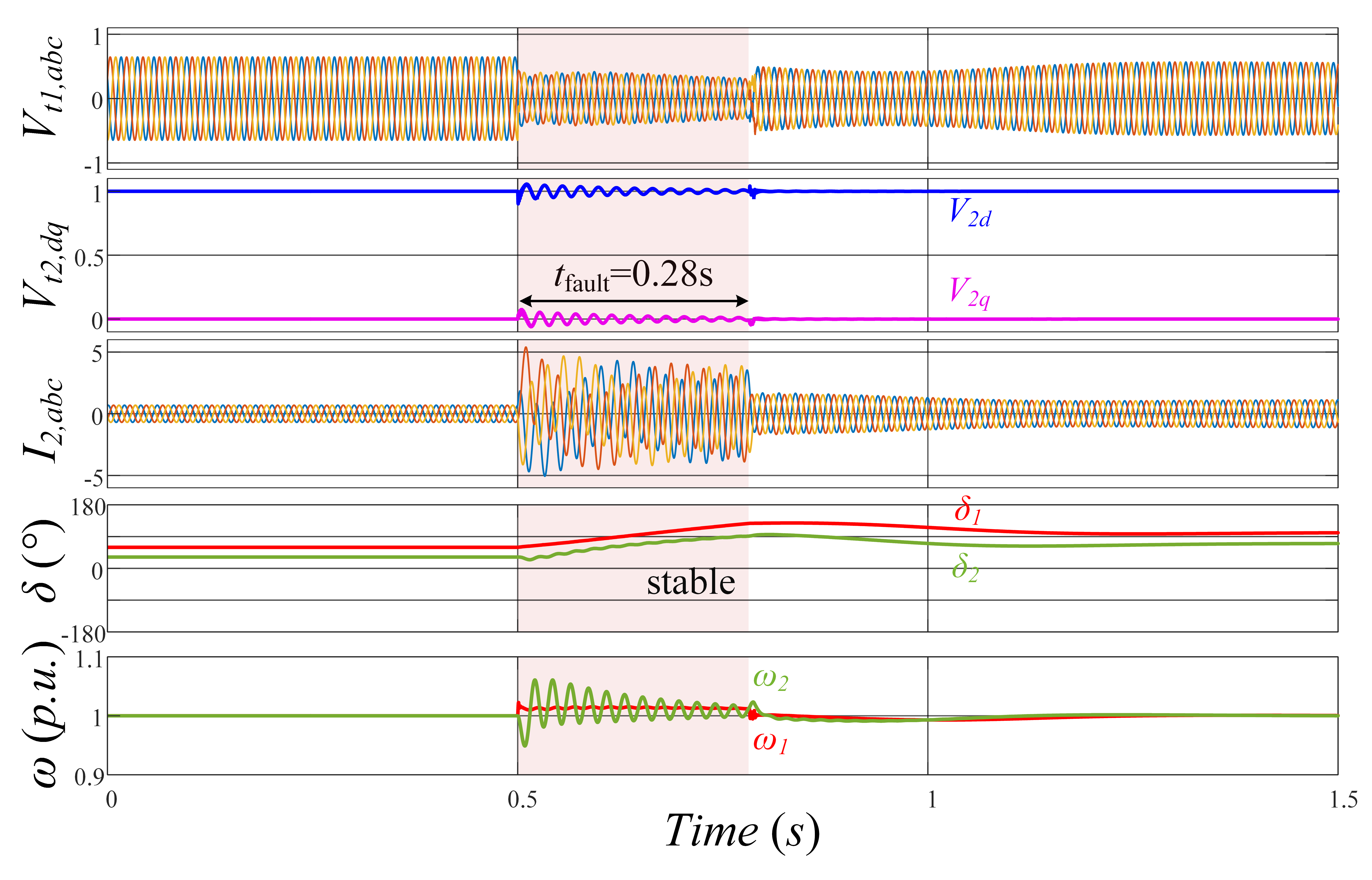
For [see Figure 6(a)(b)], the fault-on trajectory begins from the pre-fault SEP. If the fault duration is s, the system remains stable. However, with a fault duration of seconds, the post-fault trajectory fails to converge to its original SEP, resulting in instability. Time-domain simulation results for these scenarios are shown in Figure 7. Despite the post-fault trajectory potentially converging to a periodic SEP (mathematically stable), it is considered unstable in practical engineering due to phenomena like pole slipping [26, 27]. This can lead to serious consequences such as failure of distance protection [28, 29], reverse power flow in inverters [21], over-voltage, and voltage oscillations [30]. Although not the primary focus of this paper, a brief analysis is provided to explain the implications. The ratio of the fault current from the grid side () and the inverter side () for is shown in Figure 7(c). At time 0.7s, the angle of leads by approximately 90 degrees, which can result in the misoperation of Relay 41, as noted in [28]. Additionally, the impedance measurement by Relay 1 is shown in Figure 7(c), with the measured impedance becoming capacitance, signaling a fault in the transmission line . During this pole-slipping process, the IBR will suffer from reverse power injection which is not permissible.
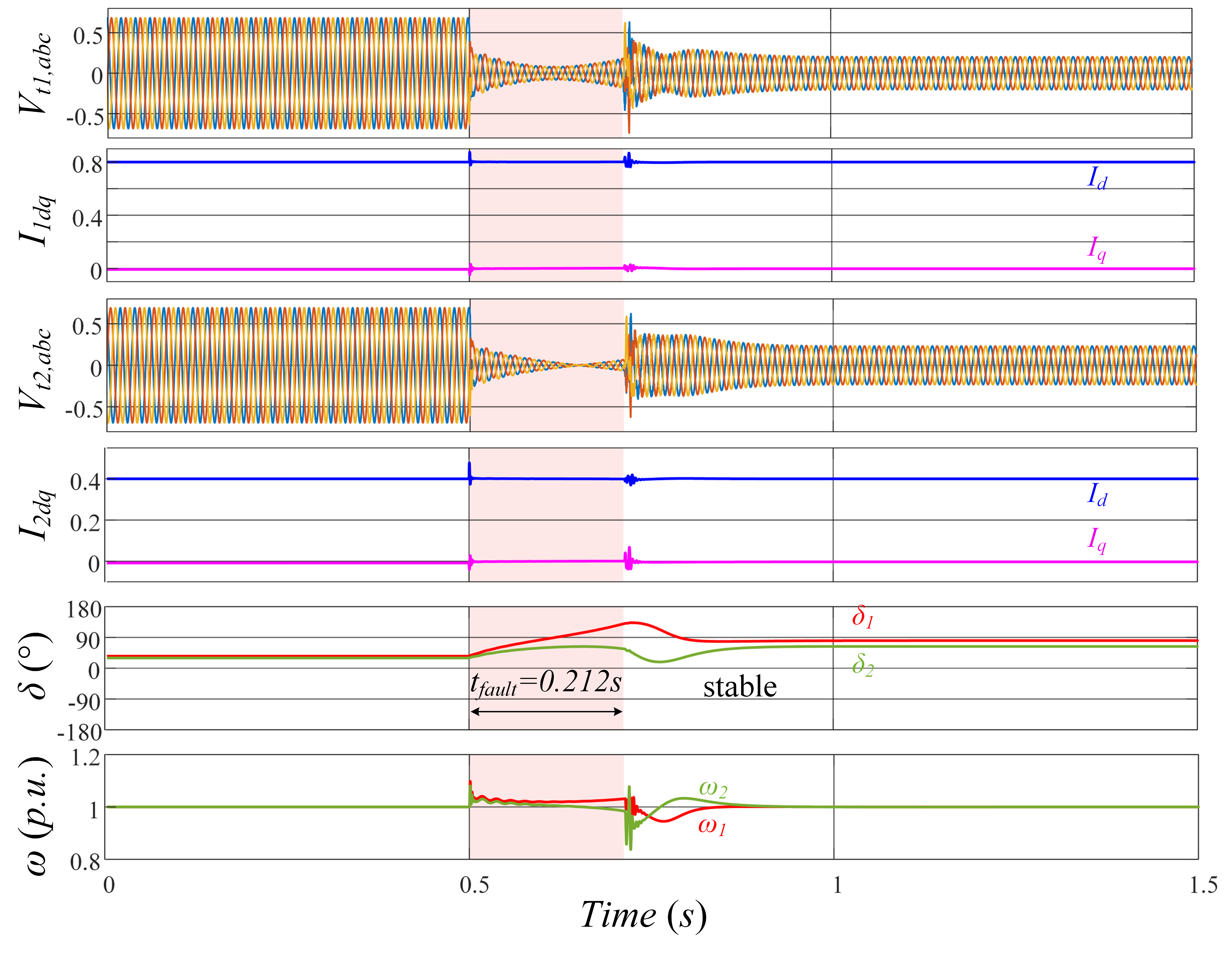
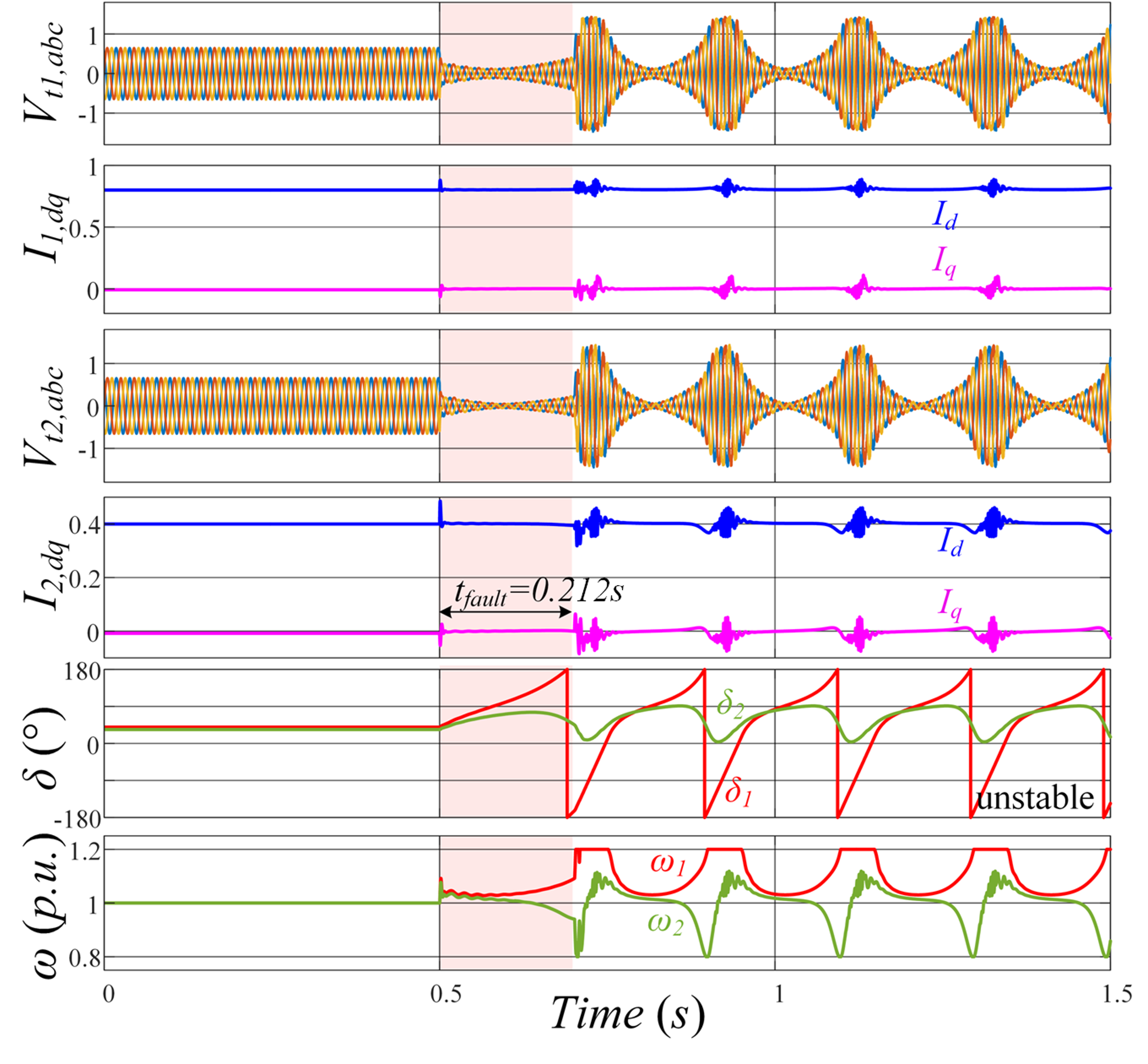
For [see Figure 6(c)(d)], if the fault duration is seconds, the system remains stable, with the post-fault trajectory (blue line) converging to the post-fault SEP. However, if seconds, the post-fault trajectory converges to SPO. In this case, diverges to infinity, while oscillates around its SEP, which is a different instability mode from the case when . This behavior is also captured in the EMT time-domain simulations in Figure 8.
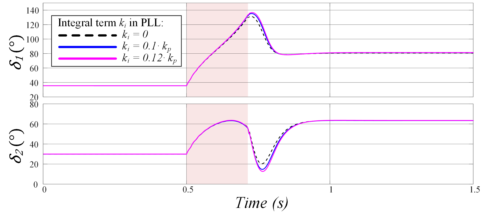
The validation of the reduced-order PLL model is presented in Figure 9. The results demonstrate that when , the angle trajectory closely matches the case where . Furthermore, under the critical fault duration time , which provides a more conservative estimate than the actual Critical Clearing Time (CCT), system stability is maintained even for . This supports the approximation of the PLL as a first-order system in the analysis.

IV-B Combination of IBR1 as a GFL inverter and IBR2 as a GFM inverter or GSP inverter
This section investigates the effect of voltage support on the transient stability of a system that includes a GFL inverter. As illustrated in Figure 5, IBR1 is configured as a GFL inverter, while IBR2 is set either as a GFM inverter or a GSP inverter. The transmission line parameters are and post-fault impedance . In this scenario, IBR2 works as STAtCOM, with a relatively small connection impedance and small active power. Detailed system parameters are provided in Table A2 (see Appendix B).
IV-B1 Comparison between GFL inverters with TVC and GFM inverters
According to Equations (7) and (8), when is large, both the GFM inverter and the GSP inverter exhibit similar dynamics. For a fair comparison, if IBR2 is realized as a GSP inverter, its PLL gain is set to , ensuring that the equivalent gain of IBR2, in general expression (12), remains consistent, whether it operates as a GFM or a GSP inverter in this section. A three-phase-to-ground fault is triggered at 0.5s, with the fault located 0.8 of the distance along from the infinite bus.
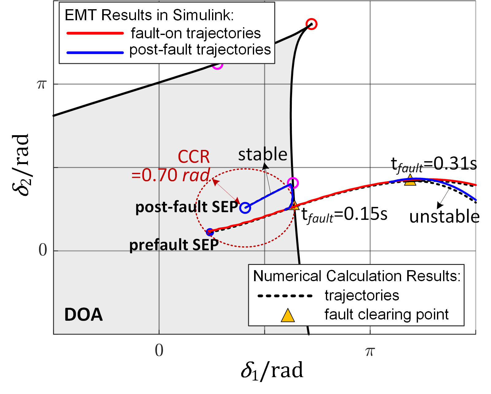
The phase portraits of the system before, during, and after the fault, with IBR2 realized by either GFM inverters or GSP inverters, are shown in Figure 10. The grey-shaded area, enclosed by the solid black line, represents the DOA. Dashed black lines indicate the trajectories of the two IBRs obtained from numerical calculations, while yellow triangles mark the fault-clearing points. Red solid lines correspond to fault-on trajectories from EMT simulations, and blue solid lines show post-fault trajectories under different fault-clearing times. As seen in Figure 10, EMT simulation results closely match their corresponding numerical calculations.
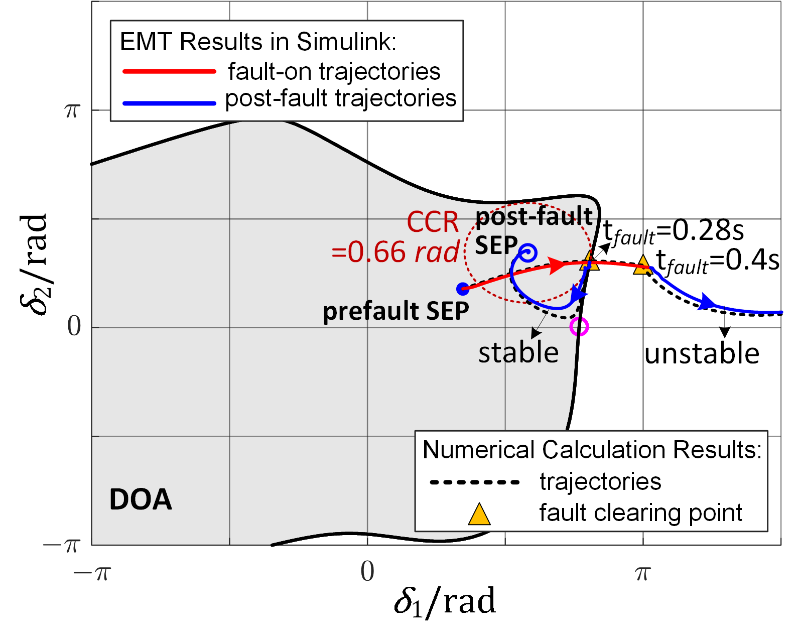

In Figure 10(a), IBR2 operates as a GFM inverter, and CCR is 0.65 rad, and CCT estimated by CCR is 0.28s. When is set to this value, the post-fault trajectory from the EMT simulation converges to the post-fault SEP, confirming the conservatives of . The corresponding time-domain results are shown in Figure 11(a). However, when the fault duration is extended to s, the trajectory does not converge to the SEP, as depicted in Figure 11(b). Additionally, in Figure 11(c), the phase difference between the currents through Relay 41 and Relay 42, denoted as and , exceeds and approaches , which is not permittable since it would trigger misoperation of the relays and failure of distance protection [28].
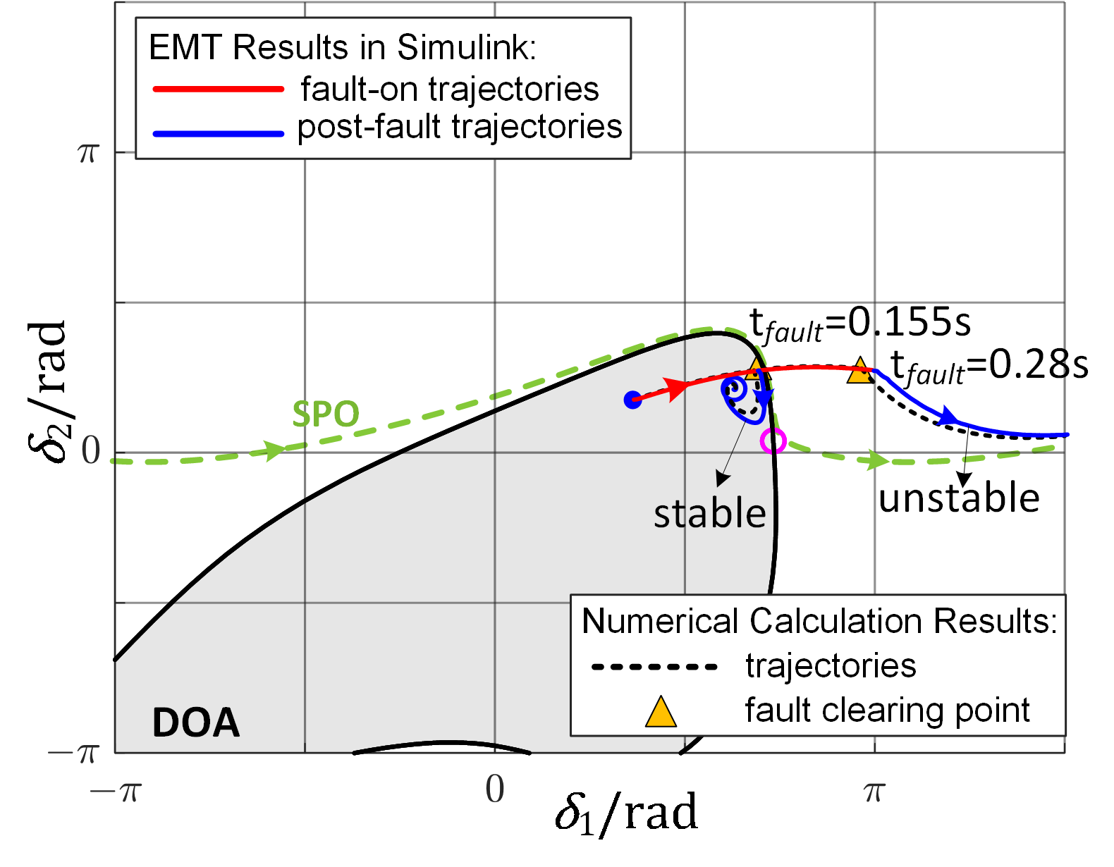
In Figure 10(b), IBR2 is configured as a GSP inverter, with a small TVC droop coefficient, . It should be noted that presence of IBR2 providing voltage support, the system cannot maintain stability, as no SEP exists. Compared to Figure 10(a), the CCR is much smaller which is 0.27 rad, and is 0.155s. In Figure 10(b), there exists an SPO outside the DOA as plotted in green dashed curves. If , the trajectory converges to this SPO, rendering the system unstable. The corresponding time domain results, shown in Figure 12(a), demonstrate the divergence of to positive infinity and oscillation of .
In Figure 10(c), the DOA and CCR are expanded when is increased to 4. The CCR becomes comparable to that of the system in which IBR2 operates as a GFM inverter, with a value of and of . However, the system with the GFM inverter demonstrates a larger transient stability margin along the -axis. For instance, when , the system loses stability in this scenario, whereas it still remains stable when using the GFM inverter, as illustrated in Figure 10(a) and Figure 10(c). The time-domain results for are presented in Figure 12(b), showing that a higher provides enhanced voltage support, maintaining the terminal voltage of IBR2 even under severe fault conditions.
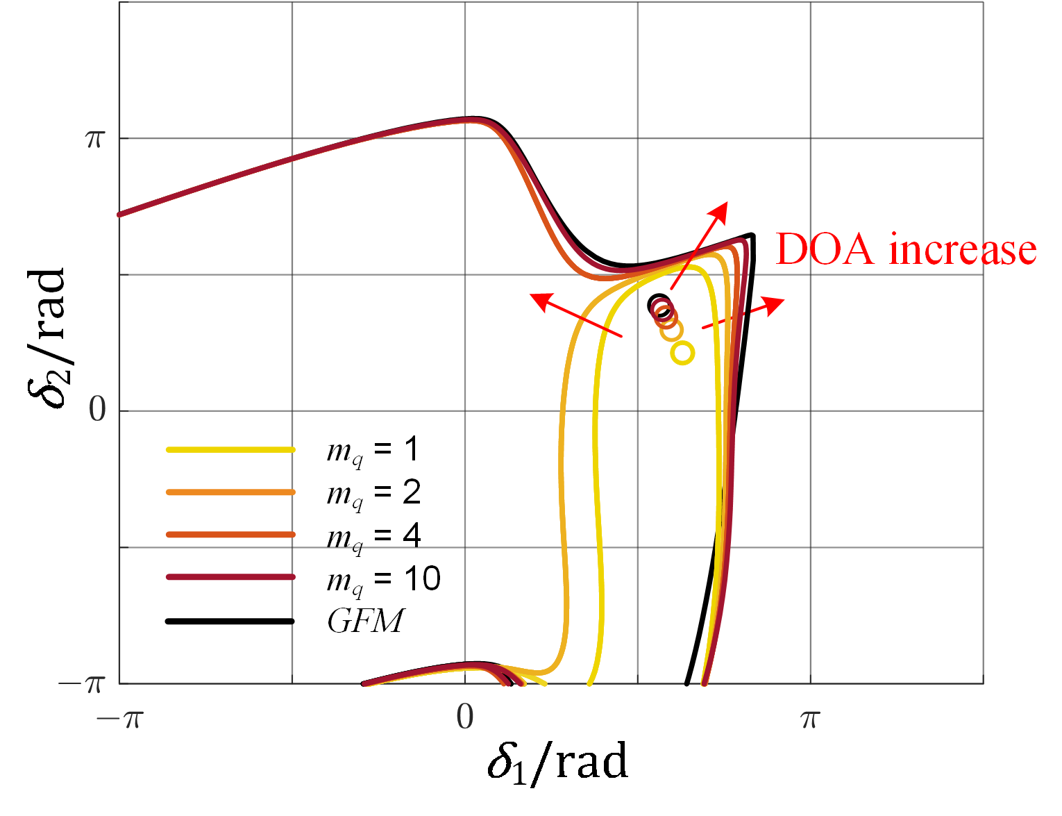
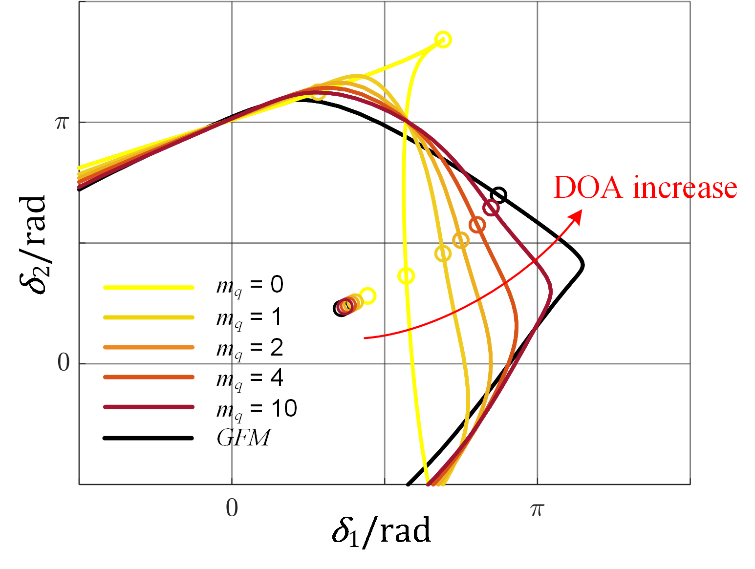
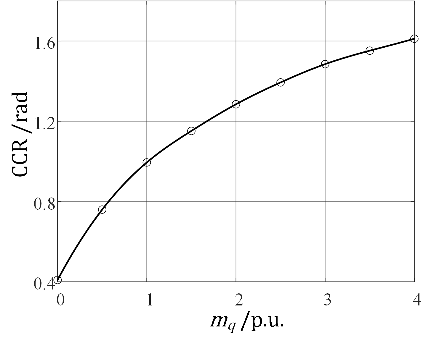
Figure 13 illustrates the DOA of the GSP inverters under different TVC droop coefficients and PLL gain is plotted. As increases, the DOA expands, improving the system’s transient stability. Under large , the DOA is very near the DOA of the system where IBR2 is GFM inverter. Especially, if is large enough and the bandwidth of the PLL2 is high, the DOA becomes comparable to that of a system with a GFM inverter (depicted by the black line in Figure 13(b)). This indicates that a GFL inverter with voltage droop control can mimic the behavior of a GFM inverter when the PLL dynamics are fast and the TVC droop coefficient is large.
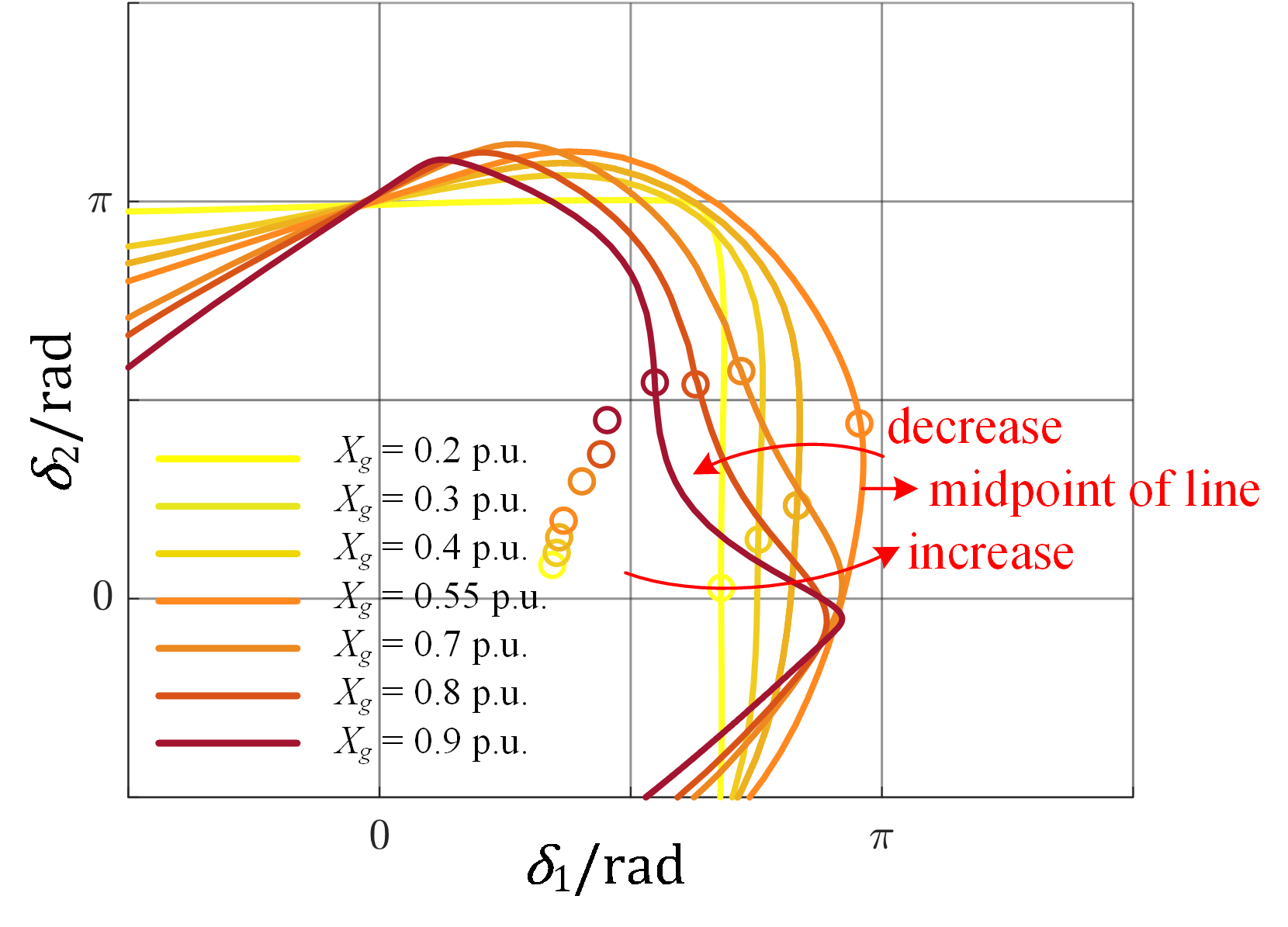
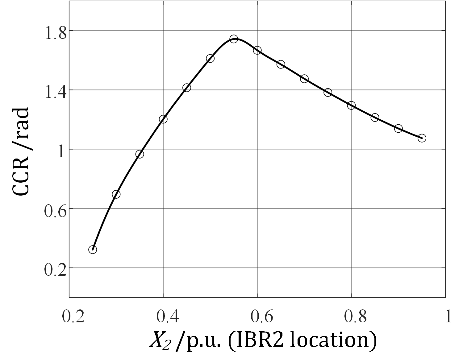
IV-B2 Impact of the location of the inverter which provides voltage support
The impact of varying the location (connection point) of the IBR2 which acts as STATCOM and provides voltage support on the DOA and CCR was further investigated. The post-fault system is analyzed herein, where the post-fault impedance and varied but the total transmission line impedance () is kept constant. Herein, the remote fault of the power grid is simulated, that is, the voltage sag fault of 0.1 p.u. is set at the infinite bus instead in the post-fault system, and the fault duration is set to 0.1s and 0.25s.
The results are illustrated in Figure 14 with the left column for a GFM inverter and the right column for a GSP inverter. The top row is the IBR2 near the inverter and moves further way in the middle and bottom rows. Examining Figure 14 shows that, regardless of whether the IBR2 is GFM or GSP inverter when it is placed in the middle of the transmission line, it is most beneficial to the transient stability of the system. When IBR2 is too near to the grid, its ability to improve voltage regulation is diminished because of proximity to an infinite bus. In the extreme case, when it is connected to the grid directly, there would be no interaction between the IBR2 and the IBR. The IBR2 must absorb active power from IBR1 and transfer it to the grid. Conversely, if the IBR2 is positioned too close to IBR1, the impedance between the IBR2 and the grid denoted as , becomes too large. This results in reduced transmission capacity to the grid and can lead to instability in the IBR2 itself. As illustrated in Figure 14(a)(b), SEP is very close to the upper boundary of DOA, which results in smaller CCT and CCR. Notably, when the IBR2 is placed at the same location as IBR1, the system lacks EP. Additionally, it is important to highlight that without the IBR2, directly applying TVC control to IBR1 results in system instability. This indicates that voltage control, while ineffective for improving the stability of the IBR itself, can enhance the stability of other IBRs.
p.u., p.u.
p.u., p.u.
p.u., p.u.
p.u., p.u.
p.u., p.u.
IV-C Combination of IBR1 as a GFM inverter and IBR2 as a GSP inverter
This section investigates the impact of voltage support provided by a GFL inverter with TVC on the transient stability of a GFM inverter. As illustrated in Figure 5, IBR1 is configured as a GFM inverter, feeding power to the grid via the transmission line p.u. The output power of IBR1 is set to p.u. Meanwhile, IBR2 is configured as a GFL inverter with TVC, which provides voltage support and is connected to the transmission line through p.u. Detailed system parameters are provided in Table A3 (see Appendix B).
At s, a severe three-phase-to-ground fault occurs at 80% of the distance along the transmission line from the infinite bus. The droop coefficient of the TVC, , is set to 0 (without TVC) in Figure 15(a), 2 in Figure 15(b), and 4 in Figure 15(c). The EMT simulation results are presented in Figure 15, where the red solid lines represent fault-on trajectories from EMT simulations, and the blue solid lines show post-fault trajectories. The CCT estimated by CCR is s, s, and s, respectively. EMT simulations under these fault clearing times confirm stability for the corresponding , demonstrating that the geometric method proposed in this paper closely matches the EMT simulation results, providing accurate and conservative CCR and CCT estimations.
As shown in Figure 15, increasing leads to a corresponding increase in CCR, thereby enhancing the system’s transient stability. Particularly, in Figure 15(a), the transient stability margin is too small without TVC, making the system prone to instability. In this sense, the TVC is also beneficial for GFM inverter in the system,
Figure 16(a)(b) shows the change in DOA and CCR with increasing , while other system parameters remain constant. Under a large , the system’s stability domain approaches that of a system where IBR2 is replaced by a GFM inverter, indicating that a higher makes the GSP inverter exhibit dynamics similar to a GFM inverter. Although the large in the GSP inverter enhances transient stability, it also reduces the bandwidth of the TVC, to ensure small-signal stability [31], making high impractical. Thus, GFM inverters remain superior to GSP inverters. Figure 16(c)(d) illustrates the effect of the GSP inverter’s location, with TVC, on the DOA. The total impedance of the transmission line for IBR1, , is kept constant at 1.1 p.u. The results show that when IBR2 is placed too close to either IBR1 or the infinite bus, the DOA decreases. The DOA and CCR is maximized when , consistent with the conclusions drawn in Section IV-B2.
V Conclusions
This paper demonstrates the non-existence of a global energy function for systems containing GFL inverters and discusses the difficulties in transient stability analysis that follow from that non-existence. To overcome these challenges, a manifold method based on manifold theory was applied to precisely determine the DOA which defines the limit of transient stable operation. To evaluate the transient stability of systems of multiple inverters, a new assessment metric termed the CCR has been proposed. A comparison was made between a GFL inverter with TVC, which is termed a GSP inverter in this paper, and a GFM inverter, and it was found that when the droop coefficient in TVC is sufficiently large, the dynamic of the system and the DOA is approaching to when the GSP inverter is replaced by GFM inverter. When one IBR is configured as STATCOM, realized by either a GSP or GFM inverter, improved voltage control is observed if it is configured as a GFM inverter instead of a GFL inverter. In systems where one IBR is a GFM inverter and the other acts as a STATCOM realized by GSP inverters, higher leads to greater transient stability, and the GSP inverter’s dynamics approach those of the GFM inverter. Finally, placing the STATCOM at the midpoint of the transmission line provides the best transient stability.
Appendix A Expression of Nonlinear Differential Equations in The Two-IBR System
A-A The expressions of the impedance used in Section II-B
| (15) |
| (16) |
| (17) |
A-B The derivation and expression of Equation (8)
The TVC equation (3b) can be expanded in detail as (18), under the case when IBR1 is a GFL inverter and IBR2 is a GSP inverter.
|
|
(18) |
where is the droop coefficient in TVC, and the -axis voltage and its voltage reference of the GSP inverter (IBR2) are denoted as and respectively. Combining , (6) and (18), the equations can be rearranged as
|
|
(19) |
Equation (19) can then be simplified to (8) where
| (20) | ||||
A-C The derivation and expression of Equation (10)
The TVC equation (3b) can be expanded in detail as (21), under the case when IBR1 is a GSP inverter and IBR2 is a GFM inverter.
|
|
(21) |
where is the droop coefficient in TVC, and the -axis voltage and its voltage reference of the GFL inverter with voltage control (IBR1) are denoted as and respectively. Combining , (7) and (21), the equations can be rearranged as
|
|
(22) |
Equation (22) can then be simplified to (10) where
|
|
(23) |
Appendix B Parameters in Simulations
| Parameters | Value (p.u.) |
| Base frequency | 50 Hz |
| Grid voltage | 1 |
| DC voltage | 2.5 |
| LCL Filter impedance | |
| LCL Filter capacitance | |
| Inner current control loop bandwidth | 1 kHz |
| PLL controller of IBR1 | |
| PLL controller of IBR1 | |
| PLL controller of IBR2 | |
| PLL controller of IBR2 | |
| Frequency limit of PLL | rad |
| Current reference of IBR1 | 0.8 |
| Current reference of IBR2 | 0.4 |
| Line impedance | 0.2j+0.002 |
| Line impedance | 0.2j+0.002 |
| Line impedance | 0.35j or 0.4j |
| Fault resistance | 0.02 |
| Parameters | Value (p.u.) |
| Base frequency | 50 Hz |
| Grid voltage | 1 |
| Impedance | 0.5j+0.025 |
| Impedance (include virtual one) | 0.1j+0.002 |
| Impedance | 0.6j+0.03 |
| Fault resistance | 0.001 |
| Fault position (from the infinite bus) | 0.8 |
| IBR1 - GFL | |
| Inner current control loop bandwidth | 1 kHz |
| PLL controller | |
| PLL controller | |
| Frequency limit of PLL | |
| Current reference | 1 |
| DC voltage | 2.5 |
| LCL filter impedance | 0.2j+0.02 |
| LCL filter capacitance | 0.01 |
| IBR2 - GFM | |
| droop gain | |
| Power reference | 0.6 in SectionIV-B1, 0 in SectionIV-B2 |
| Voltage reference | 1 |
| Inner voltage control loop bandwidth | 200 Hz |
| Inner current control loop bandwidth | 1 kHz |
| LCL filter impedance | 0.2j+0.02 |
| LCL filter capacitance | 0.1 |
| Current limit | 2 |
| IBR2 - GSP | |
| TVC droop | 1 or 4 in SectionIV-B1, 2 in SectionIV-B2 |
| Voltage reference | 1 |
| Current reference | 0.6 in SectionIV-B1, 0 in SectionIV-B2 |
| TVC bandwidth | |
| PLL controller |
| Impedance | 0.5j+0.025 |
| Impedance | 0.1j+0.002 |
| Impedance | 0.6j+0.03 |
| Fault resistance | 0.001 |
| Fault position (from the infinite bus) | 0.8 |
| IBR1 - GFM | |
| droop gain | |
| Power reference | 0.8 |
| Voltage reference | 1 |
| Inner voltage control loop bandwidth | 200 Hz |
| Inner current control loop bandwidth | 1 kHz |
| Current limit | 2 |
| IBR2 - GFL with TVC | |
| TVC droop | 0, 2, or 4 |
| Voltage reference | 1 |
| Current reference | 0.2 |
| TVC bandwidth | |
| PLL controller | |
| PLL controller |
References
- [1] Y. Gu and T. C. Green, “Power system stability with a high penetration of inverter-based resources,” Proceedings of the IEEE, 2022.
- [2] X. Wang, M. G. Taul, H. Wu, Y. Liao, F. Blaabjerg, and L. Harnefors, “Grid-synchronization stability of converter-based resources—an overview,” IEEE Open Journal of Industry Applications, vol. 1, pp. 115–134, 2020.
- [3] X. He and H. Geng, “Pll synchronization stability of grid-connected multiconverter systems,” IEEE Transactions on Industry Applications, vol. 58, no. 1, pp. 830–842, 2022.
- [4] H.-D. Chiang, Direct methods for stability analysis of electric power systems: theoretical foundation, BCU methodologies, and applications. John Wiley & Sons, 2011.
- [5] H.-D. Chiang and L. F. Alberto, Stability regions of nonlinear dynamical systems: theory, estimation, and applications. Cambridge University Press, 2015.
- [6] H. Chiang, “Study of the existence of energy functions for power systems with losses,” IEEE Transactions on Circuits and Systems, vol. 36, no. 11, pp. 1423–1429, 1989.
- [7] H. R. Pota and P. J. Moylan, “A new lyapunov function for interconnected power systems,” in Proceedings of the 28th IEEE Conference on Decision and Control,. IEEE, 1989, pp. 2181–2185.
- [8] N. G. Bretas and L. F. Alberto, “Lyapunov function for power systems with transfer conductances: extension of the invariance principle,” IEEE Transactions on Power Systems, vol. 18, no. 2, pp. 769–777, 2003.
- [9] Y. Xue, T. Van Custem, and M. Ribbens-Pavella, “Extended equal area criterion justifications, generalizations, applications,” IEEE Transactions on Power Systems, vol. 4, no. 1, pp. 44–52, 1989.
- [10] X. Fu, M. Huang, S. Pan, and X. Zha, “Cascading synchronization instability in multi-vsc grid-connected system,” IEEE Transactions on Power Electronics, vol. 37, no. 7, pp. 7572–7576, 2022.
- [11] X. Yi, Y. Peng, Q. Zhou, W. Huang, L. Xu, Z. J. Shen, and Z. Shuai, “Transient synchronization stability analysis and enhancement of paralleled converters considering different current injection strategies,” IEEE Transactions on Sustainable Energy, vol. 13, no. 4, pp. 1957–1968, 2022.
- [12] C. Shen, Z. Shuai, Y. Shen, Y. Peng, X. Liu, Z. Li, and Z. J. Shen, “Transient stability and current injection design of paralleled current-controlled vscs and virtual synchronous generators,” IEEE Transactions on Smart Grid, vol. 12, no. 2, pp. 1118–1134, 2020.
- [13] S. P. Me, M. H. Ravanji, M. Z. Mansour, S. Zabihi, and B. Bahrani, “Transient stability of paralleled virtual synchronous generator and grid-following inverter,” IEEE Transactions on Smart Grid, 2023.
- [14] Y. Xue, Z. Zhang, N. Zhang, W. Hua, G. Wang, and Z. Xu, “Transient stability analysis and enhancement control strategies for interconnected ac systems with vsc-based generations,” International Journal of Electrical Power & Energy Systems, vol. 149, p. 109017, 2023.
- [15] Y. Wang, D. Zhu, Y. Yang, X. Zou, J. Hu, and Y. Kang, “Fixed angle difference control for multi-converter grid-connected system to improve transient stability during grid faults,” in 2023 IEEE 6th International Electrical and Energy Conference (CIEEC). IEEE, 2023, pp. 4351–4356.
- [16] J. Zhao, M. Huang, and X. Zha, “Transient stability analysis of grid-connected vsis via pll interaction,” in 2018 IEEE International Power Electronics and Application Conference and Exposition (PEAC). IEEE, 2018, pp. 1–6.
- [17] M. Dellnitz and A. Hohmann, “A subdivision algorithm for the computation of unstable manifolds and global attractors,” Numerische Mathematik, vol. 75, pp. 293–317, 1997.
- [18] Z. Yang, R. Ma, S. Cheng, and M. Zhan, “Nonlinear modeling and analysis of grid-connected voltage-source converters under voltage dips,” IEEE Journal of Emerging and Selected Topics in Power Electronics, vol. 8, no. 4, pp. 3281–3292, 2020.
- [19] M. G. Taul, C. Wu, S.-F. Chou, and F. Blaabjerg, “Optimal controller design for transient stability enhancement of grid-following converters under weak-grid conditions,” IEEE Transactions on Power Electronics, vol. 36, no. 9, pp. 10 251–10 264, 2021.
- [20] H. Wu and X. Wang, “Design-oriented transient stability analysis of pll-synchronized voltage-source converters,” IEEE Transactions on Power Electronics, vol. 35, no. 4, pp. 3573–3589, 2019.
- [21] Y. Li and Y. Gu, “Whole-system first-swing stability of inverter-based inertia-free power systems,” arXiv preprint arXiv:2207.03292, 2022.
- [22] C. Zhao, D. Sun, H. Nian, and Y. Fan, “Reactive power compensation control of pv systems for improved power transfer capability in weak grid,” in 2020 12th IEEE PES Asia-Pacific Power and Energy Engineering Conference (APPEEC). IEEE, 2020, pp. 1–5.
- [23] E. Netz, “Grid code—high and extra high voltage. e. on netz gmbh,” Tech. Rep, 2006.
- [24] X. Wang, H. Wu, X. Wang, L. Dall, and J. B. Kwon, “Transient stability analysis of grid-following vscs considering voltage-dependent current injection during fault ride-through,” IEEE Transactions on Energy Conversion, pp. 1–13, 2022.
- [25] Y. Zhang, Y. Li, Y. Gu, and T. C. Green, “Consideration of control-loop interaction in transient stability of grid-following inverters using bandwidth separation method,” in 2023 11th International Conference on Power Electronics and ECCE Asia (ICPE 2023-ECCE Asia). IEEE, 2023, pp. 1294–1301.
- [26] J. Zaborszky, G. Huang, B. Zheng, and T.-C. Leung, “On the phase portrait of a class of large nonlinear dynamic systems such as the power system,” IEEE Transactions on Automatic Control, vol. 33, no. 1, pp. 4–15, 1988.
- [27] X. He, S. Pan, and H. Geng, “Transient stability of hybrid power systems dominated by different types of grid-forming devices,” IEEE Transactions on Energy Conversion, vol. 37, no. 2, pp. 868–879, 2022.
- [28] Y. Fang, K. Jia, Z. Yang, Y. Li, and T. Bi, “Impact of inverter-interfaced renewable energy generators on distance protection and an improved scheme,” IEEE Transactions on Industrial Electronics, vol. 66, no. 9, pp. 7078–7088, 2019.
- [29] J. C. Quispe H, H. Villarroel-Gutiérrez, and E. Orduña, “Analyzing short-circuit current behavior caused by inverter-interfaced renewable energy sources. effects on distance protection,” in 2020 IEEE PES Transmission $ Distribution Conference and Exhibition - Latin America (T&D LA), 2020, pp. 1–6.
- [30] X. Wang, H. Wu, and X. Wang, “Transient overvoltage analysis of grid-following vscs during fault recovery,” in 2023 11th International Conference on Power Electronics and ECCE Asia (ICPE 2023-ECCE Asia). IEEE, 2023, pp. 2404–2409.
- [31] L. Huang, H. Xin, Z. Li, P. Ju, H. Yuan, Z. Lan, and Z. Wang, “Grid-synchronization stability analysis and loop shaping for pll-based power converters with different reactive power control,” IEEE Transactions on Smart Grid, vol. 11, no. 1, pp. 501–516, 2020.