Deep Variational Sequential Monte Carlo for High-Dimensional Observations

Abstract

SMC, or particle filtering, is widely used in nonlinear state-space systems, but its performance often suffers from poorly approximated proposal and state-transition distributions. This work introduces a differentiable particle filter that leverages the unsupervised variational sequential Monte Carlo (SMC) objective to parameterize the proposal and transition distributions with a neural network, designed to learn from high-dimensional observations. Experimental results demonstrate that our approach outperforms established baselines in tracking the challenging Lorenz attractor from high-dimensional and partial observations. Furthermore, an evidence lower bound based evaluation indicates that our method offers a more accurate representation of the posterior distribution.

I Introduction

State-space estimation in dynamical systems, particularly for nonlinear systems, is a prevalent issue in statistical signal processing. Classical filters, such as the Kalman filter (KF) [1], compute the posterior state distribution based on prior observations, offering state point estimates and uncertainty quantification. The KF is optimal for linear Gaussian systems, with variants like the extended Kalman filter (EKF) [2] and unscented Kalman filter (UKF) [3] handling nonlinear systems.

Particle filtering, or SMC, represents the posterior state distribution of a stochastic process using particles, based on noisy or partial observations. This method accommodates nonlinear state-space models, handles arbitrary noise and initial state distributions, and enables posterior sampling without relying on strong Gaussian assumptions. However, traditional particle filters, such as the bootstrap particle filter (BPF) [4], often use poorly approximated proposal distributions, making them less effective in high-dimensional systems [5]. There exist particle filter variants that provide more efficient sampling in high-dimensional spaces [6, 7, 8, 9, 10], but they often require extensive domain knowledge.

DPF provide a way to propagate gradients through the normally non-differentiable resampling step [11]. Consequently, this opens up the possibility of using neural networks to parameterize the probability distributions of the particle filter, in particular the state transition and proposal distribution. Corenflos et al. [12] leverage entropy-regularized optimal transport to obtain a differentiable resampling scheme, showing that this form of resampling can outperform alternative differentiable resampling schemes.

Several approaches have been developed to learn the proposal distribution using differentiable particle filters [12, 13, 14, 15, 16, 17, 18]. However, these methods rely on a supervised objective, where the true state is known and the proposal distribution is optimized towards it. Such supervised learning is restricted to settings where labeled data is available, and cannot guarantee an accurate posterior distribution. In contrast, variational sequential Monte Carlo (VSMC) [19, 20, 21] introduces an unsupervised variational objective to learn the proposal distribution of particle filters by maximizing the expected log-marginal likelihood estimate. This optimizes the particle filter using only observation data, assuming the measurement model is known and differentiable. This work extends the application of this unsupervised objective to problems involving high-dimensional observations, such as visual data. To the best of our knowledge, this approach has not previously been explored.

This paper presents the following contributions. (1) We show that the proposal and transition distributions can be learned from high-dimensional observations without ground-truth states (unsupervised) by parameterizing the distributions using neural networks and maximizing the estimated log-marginal likelihood estimate (VSMC). (2) Experimental results using the challenging Lorenz attractor show that learning the proposal and transition distributions increases evidence lower bound (ELBO) based performance and tracking performance. (3) We show that the proposed method outperforms common alternative filtering techniques and baselines including the EKF, BPF and a supervised regression model.

The rest of this paper is organized as follows. Section II provides the signal model and particle filter background, while Section III introduces our neural network-based methodology for proposal learning from high-dimensional observations. In Section IV, we present experiments conducted on high-dimensional image data from the Lorenz attractor, with the corresponding results detailed in Section V. Finally, we conclude in Section VI.

II Background

II-A Signal model

We consider a dynamical, possibly non-linear, continuous state-space model in discrete time $t\in\mathbb{Z}$. The state variables $\mathbf{z}_{t}$ evolve using the evolution function $\mathbf{f}$, given by

$$\begin{array}[]{ll}\mathbf{z}_{t}=\mathbf{f}\left(\mathbf{z}_{t-1}\right)+\mathbf{e}_{t},&\mathbf{z}_{t}\in\mathbb{R}^{d_{z}},\end{array}$$ (1)

where $\mathbf{e}_{t}$ is the state noise. The observation vectors $\mathbf{y}_{t}$ are high-dimensional images and are related to the state-space through the measurement function $\mathbf{h}$, given by

$$\begin{array}[]{ll}\mathbf{y}_{t}=A_{t}(\mathbf{h}\left(\mathbf{z}_{t}\right)+\mathbf{v}_{t}),&\mathbf{y}_{t}\in\mathbb{R}^{h\times w},\end{array}$$ (2)

where $\mathbf{v}_{t}$ is the observation noise, $A_{t}$ is a masking operation that will randomly observe only a proportion $P$ of the image, and the observation dimensionality is $(h\times w)\gg d_{z}$.

II-B Particle filter

A particle filter aims to estimate the posterior density of state variables $\mathbf{z}_{t}$ given observations $\mathbf{y}_{t}$ over time $t\in\{1,...,T\}$ using a set of $N$ weighted particles

$$p(\mathbf{z}_{t}\mid\mathbf{y}_{1:t})\approx\sum_{i=1}^{N}w_{t}^{i}\delta\left(\mathbf{z}_{t}-\mathbf{z}_{t}^{i}\right),$$ (3)

where $w_{t}^{i}$ is the weight of particle $i$ and $\delta$ is the Dirac delta function. The particle filter used in this paper is described in Algorithm 1 and performs the resampling step when the effective sample size $\hat{N}_{eff}$ falls below a predefined threshold $N_{T}$. For more information on particle filter algorithms, we refer the reader to[22, 5].

$\left\{w_{0}^{i}\right\}_{i=1}^{N}=\{1/N\}_{i=1}^{N}$

foreach $t\in\{1\ldots T\}$ do

    foreach $i\in\{1\ldots N\}$ do

       Sample from proposal $\mathbf{z}_{t}^{i}\sim q_{\theta}\left(\mathbf{z}_{t}^{i}~\mid~\mathbf{z}_{t-1}^{i},\mathbf{y}_{t}\right)$;

       Calc. weight $\widetilde{w}_{t}^{i}\propto w_{t-1}^{i}\frac{p\left(\mathbf{y}_{t}~\mid~\mathbf{z}_{t}^{i}\right)p_{\phi}\left(\mathbf{z}_{t}^{i}~\mid~\mathbf{z}_{t-1}^{i}\right)}{q_{\theta}\left(\mathbf{z}_{t}^{i}~\mid~\mathbf{z}_{t-1}^{i},\mathbf{y}_{t}\right)}$;

      

   

   foreach $i\in\{1\ldots N\}$ do

       Normalize weights $w_{t}^{i}=\frac{\widetilde{w}_{t}^{i}}{\sum_{j=1}^{N}\widetilde{w}_{t}^{j}}$;

      

   Compute $\hat{N}_{eff}=\left(\sum_{i=1}^{N}\left(w_{t}^{i}\right)^{2}\right)^{-1}$;

    if $\hat{N}_{eff}<N_{T}$ then

       foreach $i\in\{1\ldots N\}$ do

          $\mathbf{z}_{t}^{i}\sim\textsc{Resample}^{\color[rgb]{0,0,1}{\dagger}}(\{\mathbf{z}_{t}^{i},w_{t}^{i}\})$;  $w_{t}^{i}=\frac{1}{N}$;

         

      

   

   *Compute $\hat{p}(\mathbf{y}_{t}\mid\mathbf{y}_{1:t-1})=\frac{1}{N}\sum_{i=1}^{N}\widetilde{w}_{t}^{i}$;

   

   *Aggregate $\log\hat{p}(\mathbf{y}_{1:t})=\log\hat{p}(\mathbf{y}_{1:t-1})+\log\hat{p}(\mathbf{y}_{t}\mid\mathbf{y}_{1:t-1})$;

   

*Optimize $\operatorname*{arg\,max}_{\theta}\log\hat{p}(\mathbf{y}_{1:T})$;

*is part of VSMC

^†differentiable resampling during training and systematic resampling during inference.

Algorithm 1 Particle filter with VSMC Algorithm for a single batch of data

The BPF uses $q\left(\mathbf{z}_{t}^{i}~\mid~\mathbf{z}_{t-1}^{i},\mathbf{y}_{t}\right)=p\left(\mathbf{z}_{t}^{i}~\mid~\mathbf{z}_{t-1}^{i}\right)$ as proposal distribution, and therefore does not use observations to propose new particles. This also means that the weights of the particle filter are determined only by the likelihood $p\left(\mathbf{y}_{t}~\mid~\mathbf{z}_{t}^{i}\right)$ because the proposal and transition probabilities cancel out. However, the observations are invaluable input for the proposal distribution, particularly when the state-evolution model is not accurate or hard to estimate.

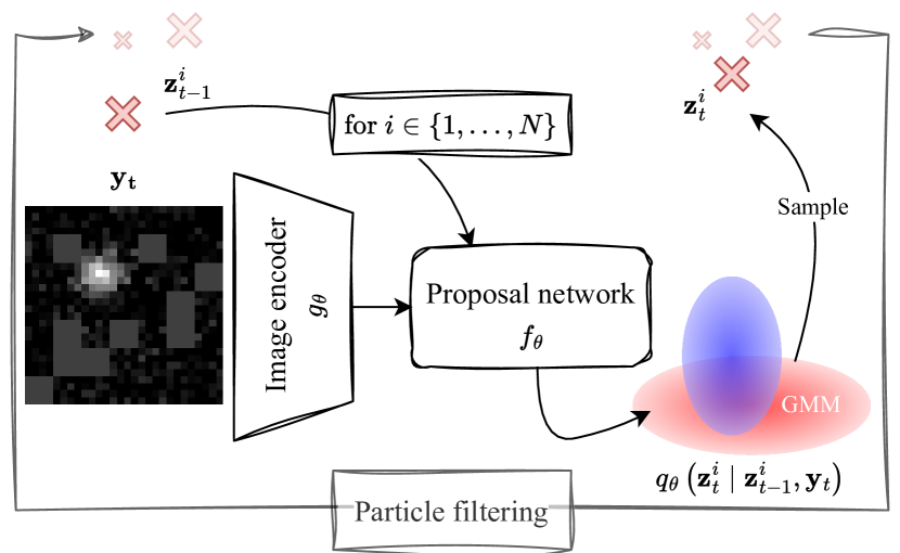
Figure 1: Illustration demonstrating the proposed method of using a parameterized proposal distribution in particle filtering.

III Methods

III-A Proposal learning

To overcome the shortcomings of the BPF, we learn the proposal distribution using the unsupervised VSMC objective. The objective function for VSMC [19, 21, 20] is the expected SMC log-marginal likelihood estimate

$$\mathbb{E}\left[\log\hat{p}\left(\mathbf{y}_{1:T}\right)\right]=\sum_{t=1}^{T}\log\left(\frac{1}{N}\sum_{i=1}^{N}\widetilde{w}_{t}^{i}\right),$$ (4)

which is proven to be a suitable variational objective and a lower bound to the true ELBO [19].

We use Gaussian mixture models for the proposal distribution

$$q_{\theta}\left(\mathbf{z}_{t}^{i}~\mid~\mathbf{z}_{t-1}^{i},\mathbf{y}_{t}\right)=\sum_{k=1}^{K}\pi_{k}^{i}\mathcal{N}\left(\boldsymbol{\mu}_{k}^{i},\boldsymbol{\sigma}_{k}^{i}I\right),$$ (5)

where $K$ represents the number of mixture components. The GMMs are parameterized by a neural network $\theta$, with parameters $\theta$ learned from data using the differentiable resampling scheme of [12]. At inference time, the faster systematic resampling scheme [23] can be used. We select GMMs for their ability to model multi-modality and their well-defined reparameterization trick [24, 25]. The parameterized proposal distribution is optimized via stochastic gradient ascent on (4) using the AdamW optimizer [26], as described in the optimization procedure of Algorithm 1. To avoid numerical errors from small log-likelihood values, the sequence length $T$ is gradually increased during training [14].

III-B Networks

The proposal distribution $q_{\theta}$ is formed by two neural networks. First, a convolutional image encoder $g_{\theta}:\mathbb{R}^{h\times w}\rightarrow\mathbb{R}^{d_{c}}$ will compress the observation image into an encoded representation. Second, a multilayer perceptron (MLP) $f_{\theta}:\mathbb{R}^{d_{z}+d_{c}}\rightarrow\mathbb{R}^{K(2d_{z}+1)}$ takes the image encoding $g_{\theta}(\mathbf{y}_{t})$ and outputs, for every particle, the parameters of a GMM as given by

$$\left\{(\pi_{1}^{i},\boldsymbol{\mu}_{1}^{i},\boldsymbol{\sigma}_{1}^{i}),\ldots,(\pi_{K}^{i},\boldsymbol{\mu}_{K}^{i},\boldsymbol{\sigma}_{K}^{i})\right\}=f_{\theta}\left(\mathbf{z}_{t-1}^{i},g_{\theta}(\mathbf{y}_{t})\right).$$ (6)

Fig. 1 illustrates the application of the neural proposal distribution. The convolution image encoder consists of three convolutional layers with a ReLU activation function. The number of convolutional features increases by a factor of 2 at each layer, while the image dimensions shrink by a factor of 2 using max pooling. Finally, a single fully connected layer maps the filters to an encoding of $d_{c}=256$ parameters. The rest of the proposal network consists of a six-layer MLP of 256 dimensions with ReLU activation. The final layer maps to a vector of size $K(2d_{z}+1)$, which corresponds to the mean, log-variance, and mixture weights of the GMM.

The transition distribution is jointly optimized and parameterized by an equivalent network architecture as the aforementioned MLP but does not take observations as input such that $f_{\phi}:\mathbb{R}^{d_{z}}\rightarrow\mathbb{R}^{K(2d_{z}+1)}$.

IV Experiments

IV-A Lorenz attractor

To demonstrate the applicability of the DPF model for high-dimensional observations, we use images generated from the Lorenz attractor [27], which exhibits chaotic nonlinear movement in 3-D space. We follow [28, 29] in projecting the state to an image using a Gaussian point spread function (PSF) as measurement function $\mathbf{h}$. The observations $\mathbf{y}_{t}$ are images of 28$\times$28 pixels. For noise distributions $\mathbf{e}_{t}$ and $\mathbf{v}_{t}$ we choose additive white Gaussian noise (AWGN) with a standard deviation of 0.5 for $\mathbf{e}_{t}$ and a standard deviation in the range of [0.1, 0.6] for $\mathbf{v}_{t}$. Here, $A_{t}$ in (2) is the identity function. Additionally, we conduct an experiment where the images are partially observed by randomly dropping 4$\times$4 pixel blocks with varying probabilities, as defined by $A_{t}$. In this experiment, AWGN is fixed to a standard deviation of 0.1. Some examples can be seen in Fig. 2.

The measurement model $p\left(\mathbf{y}_{t}~\mid~\mathbf{z}_{t}^{i}\right)$ maps the particles from the state space to the observation space using the PSF, and then calculates the pixel-wise error assuming a Gaussian distribution, with variance corresponding to the AWGN present in the images. In our experiments, the transition distribution $p\left(\mathbf{z}_{t}^{i}~\mid~\mathbf{z}_{t-1}^{i}\right)$ is considered unknown, leading to a mismatch with the simulated state transitions and adding to the complexity of the problem.

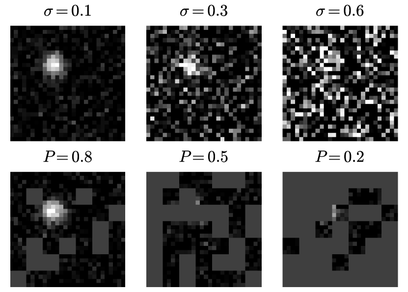
Figure 2: Example images of the Lorenz attractor (in the same position) using various noise levels with standard deviation $\sigma$ (top) and randomly dropped observations where $P$ represents the proportion of observations (bottom).

IV-B Baselines

The proposed unsupervised model was compared to several baselines, including the EKF [2], BPF [4], and a supervised neural network. The supervised network was trained to map noisy or partially observed images to an estimated coordinate using Euclidean distance as the loss function. This non-variational encoder estimates the posterior mean coordinate. It mirrors the network for the proposal distribution in Section III-B, but the final layer outputs a coordinate estimate instead of distribution parameters.

The state-space dynamics are considered to be unknown in this work. To address this, the BPF and EKF estimate velocity as part of the state and assume a constant velocity transition model. In contrast, the DPF simultaneously learns the transition and proposal distribution, allowing it to adapt to complex dynamics. Unlike the baselines, which initialize particles around the initial position using a Gaussian distribution with unit variance, the DPF initializes particles using an estimated prior distribution. This makes the DPF significantly more flexible, as it does not rely on a predefined initial position. All particle filters use $N=28$ particles except for the BPF with 280 particles. The resample threshold is always $N_{T}=\frac{N}{2}$. Validation is performed on 32 unseen sequences of 128 timesteps while the models are trained on 1024 sequences of 8 timesteps divided into batches of 32 sequences. We trained the DPF and the supervised encoder once for multiple noise levels and once for the various levels of partial observations. The DPF employs a proposal and transition distribution with $K=2$ mixture components.

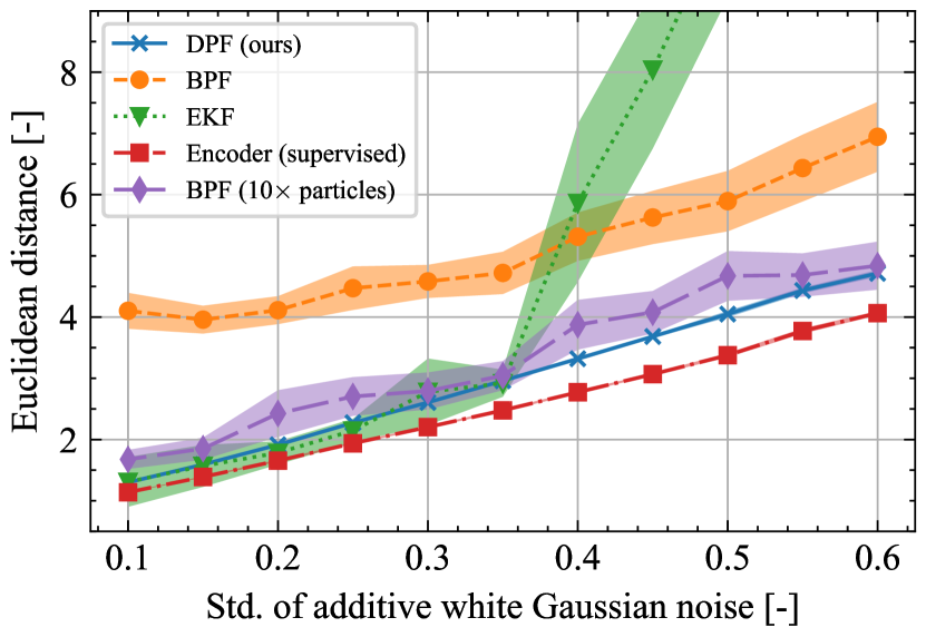
Figure 3: Tracking error of the DPF compared to the baseline methods for varying noise levels. The tracking error is computed using the Euclidean distance of the predicted location to the ground truth location. The error bars depict the 95% confidence interval calculated using 20 different seeds.

IV-C Metrics

We evaluate the accuracy of the state estimate in terms of Euclidean distance as well as the ELBO for the various filtering techniques. The ELBO can be decomposed into the likelihood of the observations and the Kullback–Leibler (KL) divergence to the prior as given by

$$\begin{split}\ln p(\mathbf{y}_{t})&\geq\mathbb{E}_{\mathbf{z}_{t}\sim q(\cdot\mid\mathbf{y}_{t})}[\ln p(\mathbf{y}_{t}\mid\mathbf{z}_{t})]\\ &-\mathbb{E}_{\mathbf{z}_{t}\sim q(\cdot\mid\mathbf{y}_{t})}\left[\ln q(\mathbf{z}_{t}\mid\mathbf{y}_{t})-\ln p(\mathbf{z}_{t})\right].\end{split}$$ (7)

The prior $p(\mathbf{z})$ is estimated by aggregating many timesteps of the Lorenz attractor and using Gaussian kernel density estimation. The particles from the SMC posterior are fitted with a Gaussian to enable sampling and evaluating arbitrary points. The likelihood and KL are estimated using Monte Carlo sampling.

In addition to evaluating the variational performance, the tracking performance is assessed using the posterior mean. The posterior mean is determined by calculating the weighted mean of the particles. Following this, the Euclidean distance is measured relative to the ground truth coordinates of the attractor.

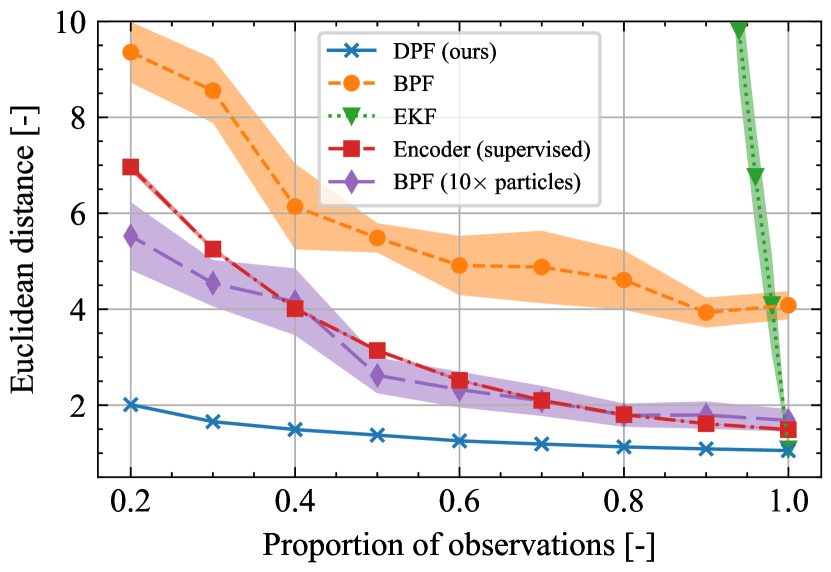
Figure 4: Tracking error of the DPF compared to the baseline methods for various levels of partial observations. The tracking error is computed using the Euclidean distance of the predicted location to the ground truth location. The error bars depict the 95% confidence interval calculated using 10 different seeds.

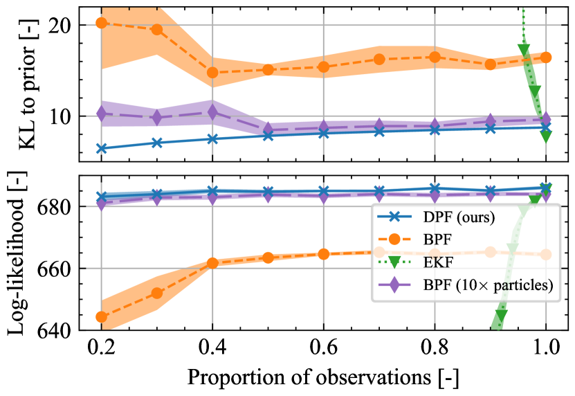
Figure 5: Decomposition of the ELBO for the DPF and the baselines for various levels of partial observations. The error bars depict the 95% confidence interval calculated using 10 different seeds.

V Results

Fig. 3 shows the tracking error as a function of the AWGN standard deviation. As anticipated, the supervised method achieves the best performance due to the fully observed image. Among unsupervised models, the DPF performs the best. Up to a standard deviation of 0.35, the EKF performs similarly to the DPF, but its error rises sharply beyond this point. Meanwhile, the BPF demonstrates stable but suboptimal performance, even when using 10 times the number of particles.

Tracking error under varying levels of dropped observations is illustrated in Fig. 4. The DPF significantly outperforms all other methods, with the supervised encoder and BPF (10$\times$ particles) being its closest competitors. With limited observations, the supervised encoder deviates from DPF due to the lack of a state-transition model. The EKF struggles with partial observations.

The ELBO decomposition in Fig. 5 reveals that the DPF reduces the KL divergence to the prior as observation uncertainty increases, while maintaining a stable log-likelihood. In contrast, the BPF with the same number of particles remains relatively stable, but drops sharply when observations fall below 40%, and the EKF deviates significantly. The figure demonstrates that the DPF provides the most accurate modeling of the posterior distribution.

VI Conclusion

We proposed an unsupervised neural augmentation of particle filters for dynamical state estimation from high-dimensional observations. Our approach leverages parameterized proposal and transition distributions and the unsupervised VSMC objective to effectively mitigate the challenge of poorly approximated proposals. It learns from high-dimensional observations without the need for ground-truth state information, showing significant improvements over established baselines on the challenging Lorenz attractor, especially in cases with limited observations. Additionally, the ELBO-based evaluation confirms that the posterior distribution is modeled more accurately.

References

- [1] R. E. Kalman, “A New Approach to Linear Filtering and Prediction Problems,” Journal of Basic Engineering, vol. 82, no. 1, pp. 35–45, Mar. 1960.
- [2] A. H. Jazwinski, Stochastic Processes and Filtering Theory. Academic Press, Jan. 1970.
- [3] S. J. Julier and J. K. Uhlmann, “New extension of the Kalman filter to nonlinear systems,” in Signal Processing, Sensor Fusion, and Target Recognition VI, vol. 3068. SPIE, Jul. 1997, pp. 182–193.
- [4] N. J. Gordon, D. J. Salmond, and A. F. M. Smith, “Novel approach to nonlinear/non-Gaussian Bayesian state estimation,” IEE Proceedings F (Radar and Signal Processing), vol. 140, no. 2, pp. 107–113, Apr. 1993.
- [5] C. A. Naesseth, F. Lindsten, and T. B. Schön, “Elements of Sequential Monte Carlo,” Mar. 2022.
- [6] A. Doucet, N. de Freitas, K. P. Murphy, and S. J. Russell, “Rao-Blackwellised Particle Filtering for Dynamic Bayesian Networks,” in Proceedings of the 16th Conference on Uncertainty in Artificial Intelligence, ser. UAI ’00. San Francisco, CA, USA: Morgan Kaufmann Publishers Inc., Jun. 2000, pp. 176–183.
- [7] P. M. Djuric, T. Lu, and M. F. Bugallo, “Multiple Particle Filtering,” in 2007 IEEE International Conference on Acoustics, Speech and Signal Processing - ICASSP ’07, vol. 3, Apr. 2007, pp. III–1181–III–1184.
- [8] P. M. Djuric and M. F. Bugallo, “Particle filtering for high-dimensional systems,” in 2013 5th IEEE International Workshop on Computational Advances in Multi-Sensor Adaptive Processing (CAMSAP). St. Martin, France: IEEE, Dec. 2013, pp. 352–355.
- [9] P. Bunch and S. Godsill, “Approximations of the Optimal Importance Density using Gaussian Particle Flow Importance Sampling,” Nov. 2014.
- [10] J. Heng, A. Doucet, and Y. Pokern, “Gibbs flow for approximate transport with applications to Bayesian computation,” Jan. 2020.
- [11] X. Chen and Y. Li, “An overview of differentiable particle filters for data-adaptive sequential Bayesian inference,” Foundations of Data Science, pp. 0–0, Tue Dec 26 00:00:00 EST 2023.
- [12] A. Corenflos, J. Thornton, G. Deligiannidis, and A. Doucet, “Differentiable Particle Filtering via Entropy-Regularized Optimal Transport,” Jun. 2021.
- [13] F. Gama, N. Zilberstein, M. Sevilla, R. Baraniuk, and S. Segarra, “Unsupervised Learning of Sampling Distributions for Particle Filters,” Feb. 2023.
- [14] B. Cox, S. Pérez-Vieites, N. Zilberstein, M. Sevilla, S. Segarra, and V. Elvira, “End-to-End Learning of Gaussian Mixture Proposals Using Differentiable Particle Filters and Neural Networks,” in ICASSP 2024 - 2024 IEEE International Conference on Acoustics, Speech and Signal Processing (ICASSP), Apr. 2024, pp. 9701–9705.
- [15] X. Chen and Y. Li, “Normalising Flow-based Differentiable Particle Filters,” Mar. 2024.
- [16] J. Li, X. Chen, and Y. Li, “Learning Differentiable Particle Filter on the Fly,” Dec. 2023.
- [17] R. Jonschkowski, D. Rastogi, and O. Brock, “Differentiable Particle Filters: End-to-End Learning with Algorithmic Priors,” May 2018.
- [18] A. Ścibior and F. Wood, “Differentiable Particle Filtering without Modifying the Forward Pass,” Oct. 2021.
- [19] C. A. Naesseth, S. W. Linderman, R. Ranganath, and D. M. Blei, “Variational Sequential Monte Carlo,” Feb. 2018.
- [20] C. J. Maddison, D. Lawson, G. Tucker, N. Heess, M. Norouzi, A. Mnih, A. Doucet, and Y. W. Teh, “Filtering Variational Objectives,” Nov. 2017.
- [21] T. A. Le, M. Igl, T. Rainforth, T. Jin, and F. Wood, “Auto-Encoding Sequential Monte Carlo,” Apr. 2018.
- [22] M. Arulampalam, S. Maskell, N. Gordon, and T. Clapp, “A tutorial on particle filters for online nonlinear/non-Gaussian Bayesian tracking,” IEEE Transactions on Signal Processing, vol. 50, no. 2, pp. 174–188, Feb. 2002.
- [23] J. Carpenter, P. Clifford, and P. Fearnhead, “Improved particle filter for nonlinear problems,” IEE Proceedings - Radar, Sonar and Navigation, vol. 146, no. 1, pp. 2–7, Feb. 1999.
- [24] A. Graves, “Stochastic Backpropagation through Mixture Density Distributions,” Jul. 2016.
- [25] M. Figurnov, S. Mohamed, and A. Mnih, “Implicit Reparameterization Gradients,” Jan. 2019.
- [26] I. Loshchilov and F. Hutter, “Decoupled Weight Decay Regularization,” Jan. 2019.
- [27] E. N. Lorenz, “Deterministic Nonperiodic Flow,” Journal of Atmospheric Sciences, Mar. 1963.
- [28] I. Buchnik, D. Steger, G. Revach, R. J. G. van Sloun, T. Routtenberg, and N. Shlezinger, “Latent-KalmanNet: Learned Kalman Filtering for Tracking from High-Dimensional Signals,” Apr. 2023.
- [29] V. Garcia Satorras, Z. Akata, and M. Welling, “Combining Generative and Discriminative Models for Hybrid Inference,” in Advances in Neural Information Processing Systems, vol. 32. Curran Associates, Inc., 2019.