Analytical closed-form solution of the Bagley-Torvik equation

Juan Luis González-Santander Alexander Apelblat
Abstract

We calculate the solution of the Bagley-Torvik equation for arbitrary initial conditions and arbitrary external force as the sum of two terms. The first one is a linear combination of exponentials with error functions, and the second one is a convolution integral whose kernel is a linear combination of exponentials with error functions. The derivation of the solution is carried out by using the Laplace transform method and the calculation of a new inverse Laplace transform. The aforementioned convolution integral can be calculated for the cases of a sinusoidal- or a potential-type external force. In addition, we calculate the asymptotic behaviour of the solution for $t\rightarrow 0^{+}$ and $t\rightarrow+\infty$. The computation of this new analytical solution is much faster and stable than other analytical solutions found in the literature.

1 Introduction

In 1984, P. J. Torvik and R. L. Bagley [1] considered the motion of a rigid plate $y\left(t\right)$ of mass $m$ and area $A$ immersed in a Newtonian fluid of infinite extent with density $\rho$ and viscosity $\mu$. This plate is connected by a massless spring of stiffness $K$ to a fixed point, where an external force $f\left(t\right)$ is applied to it for $t>0$, see Figure 1. Note that the displacement $y\left(t\right)$ of the plate is referred to the equilibrium point $\ell_{0}$ at which the weight of the plate is compensated by the force exerted by the spring and the buoyancy force experimented by the plate.

Refer to caption
Figure 1: Immersed plate in a Newtonian fluid connected by a massless spring.

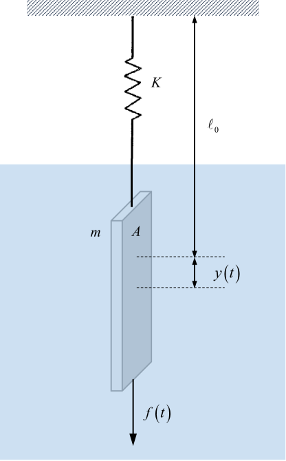
The motion of the plate is governed by the following fractional-order differential equation [2, Eqn. 8.18]:

$$a\,\,y^{\prime\prime}\left(t\right)+b\,\,_{0}^{\ast}D_{t}^{3/2}y\left(t\right)+c\,y\left(t\right)=f\left(t\right),\quad t>0,$$ (1)

where $a=m$, $b=2A\sqrt{\mu\rho}$, $c=K$ and ${}_{0}^{\ast}D_{t}^{3/2}y\left(t\right)$ denotes the Caputo fractional derivative of order $3/2$. Next, we recall the definition of the Caputo fractional derivative.

Definition 1

For $m=1,2,\ldots$, the Caputo fractional derivative of order $\alpha>0$ is defined as [3, Eqn. 1.17b]:

$${}_{0}^{\ast}D_{t}^{\alpha}g\left(t\right)=\left\{\begin{array}[]{ll}\displaystyle\frac{1}{\Gamma\left(m-\alpha\right)}\int_{0}^{t}\frac{g^{\left(m\right)}\left(\tau\right)}{\left(t-\tau\right)^{\alpha+1-m}}d\tau,&m-1<\alpha<m,\\ \displaystyle\frac{d^{m}}{dt^{m}}g\left(t\right),&\alpha=m.\end{array}\right.$$ (2)

It is worth noting that the plate-fluid system must be in an equilibrium state in order to derive (1), thus the initial velocity of the plate must be zero, i.e. $y^{\prime}\left(0\right)=0$. In the original work of Torvik and Bagley [1], they considered homogeneous initial conditions:

$$y\left(0\right)=y^{\prime}\left(0\right)=0.$$ (3)

Here, we generalize the Bagley-Torvik equation (1) for non-homogeneous initial conditions $y\left(0\right)$, $y^{\prime}\left(0\right)$. In this case, we can write the solution as

$$y\left(t\right)=y_{f}\left(t\right)+y_{c}\left(t\right),$$ (4)

where $y_{f}\left(t\right)$ takes into account the effect of the external force $f\left(t\right)$ exerted to the plate, and $y_{c}\left(t\right)$ takes into account the effect of non-homogeneous initial conditions. Note that if $f\left(t\right)=0$ and $y\left(0\right)=y^{\prime}\left(0\right)=0$, the solution of (1) is $y\left(t\right)=0$, for $t>0$. Physically speaking, this means that the plate will remain at the equilibrium point, i.e. the initial position.

Since the Bagley-Torvik equation plays a vital role in many problems of applied science and engineering, a large number of researchers show interest in its solution. In Section 2, we explain the most common analytical and numerical approaches to solve the Bagley-Torvik equation and its generalizations. Also in Section 2, we present some properties of the Mittag-Leffler function that will be needed throughout the paper. The reader will find many more references in [4] regarding the great variety of approaches found in the literature in order to solve the Bagley-Torvik equation.

It is worth noting that a fractional-order differential equation similar to (1) arises in fluid mechanics when we study the motion of a rigid sphere in the gravity field, starting from rest in a quiescent fluid. This problem was first treated by Basset [5] and since then is called Basset problem. The generalization of the Basset problem and its analytical solution via Laplace transform method is given in [6]. We will follow a similar approach in order to analytically solve (1) in this paper.

The goal of this paper is to solve the Bagley-Torvik equation given in (1) for given constants $a,b,c\in\mathbb{R}$ and arbitrary external force $f\left(t\right)$ with initial conditions $y\left(0\right),y^{\prime}\left(0\right)\in\mathbb{R}$ in closed-form. For this purpose, we derive a new Laplace transform in Section 3. In Section 4, we apply this new Laplace transform to obtain the general solution of (1), where $y_{c}\left(t\right)$ is given as a linear combination of exponentials with error functions; and where $y_{f}\left(t\right)$ is given in terms of a convolution integral. In the next two sections, we calculate $y_{f}\left(t\right)$ for particular forms of $f\left(t\right)$. Thereby, in Section 5, we consider $f\left(t\right)$ as a linear combination of potential functions; and in Section 6, as a sinusoidal function. In addition we present the asymptotic behaviour of the solution for $t\rightarrow 0^{+}$ and $t\rightarrow\infty$ in Section 7. In Section 8, we present some numerical examples in order to compare the behaviour of our solution to other approaches found in the literature. We collect our conclusions in Section 9. Finally, the calculation of some auxiliary integrals is included in Appendix A.

2 Preliminaries

As aforementioned in the Introduction, this section is devoted to presenting some properties of the Mittag-Leffler function that will be used throughout the paper, as well as to explain the most common analytical and numerical approaches in existing literature in order to solve the Bagley-Torvik equation.

2.1 Some properties of the Mittag-Leffler function

Definition 2

The one-parameter Mittag-Leffler function is defined as [7, Eqn. 3.1.1]:

$$\mathrm{E}_{\alpha}\left(z\right)=\sum_{k=0}^{\infty}\frac{z^{k}}{\Gamma\left(\alpha k+1\right)},\quad\alpha\in\mathbb{C},$$ (5)

where $\Gamma\left(z\right)$ denotes the gamma function [8, Eqn. 43:3:1].

Definition 3

The two parameter Mittag-Leffler function is defined as [7, Eqn. 4.1.1]:

$$\mathrm{E}_{\alpha,\beta}\left(z\right)=\sum_{k=0}^{\infty}\frac{z^{k}}{\Gamma\left(\alpha k+\beta\right)},\quad\mathrm{Re}\,\alpha>0,\beta\in\mathbb{C}.$$ (6)
Remark 4

Note that the one-parameter Mittag-Leffler function is a special case of the two-parameter Mittag-Leffler function, since $\mathrm{E}_{\alpha}\left(z\right)=\mathrm{E}_{\alpha,1}\left(z\right)$.

In existing literature [7, Eqn. 3.2.4], we found the reduction formula

$$\mathrm{E}_{1/2,1}\left(z\right)=\mathrm{E}_{1/2}\left(z\right)=\exp\left(z^{2}\right)\,\mathrm{erfc}\left(-z\right).$$ (7)

Also, we found the property [7, Eqn. 4.2.3]:

$$\mathrm{E}_{\alpha,\beta}\left(z\right)=\frac{1}{\Gamma\left(\beta\right)}+z\,\mathrm{E}_{\alpha,\alpha+\beta}\left(z\right).$$ (8)

From (7) and (8), and knowing that $\Gamma\left(\frac{1}{2}\right)=\sqrt{\pi}$ and $\Gamma\left(1\right)=1$ [8, Sect. 43:7], we obtain

$$\mathrm{E}_{1/2,1/2}\left(z\right)=\frac{1}{\sqrt{\pi}}+z\exp\left(z^{2}\right)\,\mathrm{erfc}\left(-z\right),$$ (9)

and

$$\mathrm{E}_{1/2,3/2}\left(z\right)=\frac{\exp\left(z^{2}\right)\,\mathrm{erfc}\left(-z\right)-1}{z}.$$ (10)

From (9) and (8), and knowing that $1/\Gamma\left(0\right)=0$ [8, Sect. 43:7], we obtain

$$\mathrm{E}_{1/2,0}\left(z\right)=z\left(\frac{1}{\sqrt{\pi}}+z\exp\left(z^{2}\right)\,\mathrm{erfc}\left(-z\right)\right).$$ (11)

Finally, from (11) and (8), and knowing that $\Gamma\left(-\frac{1}{2}\right)=-2\sqrt{\pi}$ [8, Sect. 43:7], we obtain

$$\mathrm{E}_{1/2,-1/2}\left(z\right)=\frac{1}{\sqrt{\pi}}\left(z^{2}-\frac{1}{2}\right)+z^{3}\exp\left(z^{2}\right)\,\mathrm{erfc}\left(-z\right).$$ (12)

2.2 Analytical solutions

The analytical solution of (1) given in the literature for homogeneous initial conditions (3) reads as [2, Eqns. 8.26-27], :

$$y\left(t\right)=y_{f}\left(t\right)=\int_{0}^{t}f\left(\tau\right)G\left(t-\tau\right)d\tau,$$ (13)

being

$$G\left(t\right)=\frac{1}{a}\sum_{k=0}^{\infty}\frac{\left(-1\right)^{k}}{k!}\left(\frac{c}{a}\right)^{k}t^{2k+1}\,\mathrm{E}_{1/2,2+3k/2}^{\left(k\right)}\left(-\frac{b}{a}\sqrt{t}\right),$$ (14)

and $\mathrm{E}_{\lambda,\mu}^{\left(k\right)}\left(z\right)$ the $k$-th derivative of the two-parameter Mittag-Leffler function (6).

$$\mathrm{E}_{\lambda,\mu}^{\left(k\right)}\left(z\right)=\frac{d^{k}}{dz^{k}}\mathrm{E}_{\lambda,\mu}\left(z\right)=\sum_{j=0}^{\infty}\frac{\left(j+k\right)!\,z^{j}}{j!\,\Gamma\left(\lambda j+\lambda k+\mu\right)}.$$ (15)

By using the Adomian decomposition, the solution given in (13)-(15) is obtained in [9] for the particular case $f\left(t\right)=8\left[H\left(t\right)-H\left(t-1\right)\right]$ where $H\left(t\right)$ denotes the Heaviside function. By using the Laplace transform, the solution given in (13)-(15) is obtained in [10, Example 8.2] for the particular case $f\left(t\right)=\sin t$.

In [11], we found the solution of (1) for non-homogeneous initial conditions $y\left(0\right)$, $y^{\prime}\left(0\right)$, where $y_{f}\left(t\right)$ is given by (13)-(15) and

$\displaystyle y_{c}\left(t\right)$ $\displaystyle=$ $\displaystyle y\left(0\right)\sum_{k=0}^{\infty}\frac{\left(-1\right)^{k}}{k!}\left(\frac{c}{a}\right)^{k}t^{2k}\,\mathrm{E}_{1/2,1+3k/2}^{\left(k\right)}\left(-\frac{b}{a}\sqrt{t}\right)$
$\displaystyle+y\left(0\right)\frac{b}{a}\sum_{k=0}^{\infty}\frac{\left(-1\right)^{k}}{k!}\left(\frac{c}{a}\right)^{k}t^{2k+1/2}\,\mathrm{E}_{1/2,3+3\left(k-1\right)/2}^{\left(k\right)}\left(-\frac{b}{a}\sqrt{t}\right)$
$\displaystyle+y^{\prime}\left(0\right)\frac{b}{a}\sum_{k=0}^{\infty}\frac{\left(-1\right)^{k}}{k!}\left(\frac{c}{a}\right)^{k}t^{2k+3/2}\,\mathrm{E}_{1/2,4+3\left(k-1\right)/2}^{\left(k\right)}\left(-\frac{b}{a}\sqrt{t}\right)$
$\displaystyle+y^{\prime}\left(0\right)\sum_{k=0}^{\infty}\frac{\left(-1\right)^{k}}{k!}\left(\frac{c}{a}\right)^{k}t^{2k+1}\,\mathrm{E}_{1/2,2+3k/2}^{\left(k\right)}\left(-\frac{b}{a}\sqrt{t}\right).$

Other approach to obtain an analytical solution for non-homogeneous initial conditions is given in [12]. However, this method is restricted to functions of the following type:

$$f\left(t\right)=\sum_{k=0}^{n}a_{k}\,t^{k/2}.$$ (17)

The solution is given in series form as

$$y\left(t\right)=\sum_{k=0}^{\infty}d_{k}\,t^{k/2},$$ (18)

where $d_{0}=y\left(0\right)$, $d_{1}=0$, $d_{2}=y^{\prime}\left(0\right)$, $d_{3}=0$, and

$\displaystyle d_{k+4}$ $\displaystyle=$ $\displaystyle\frac{\Gamma\left(\frac{k}{2}+1\right)\left[\phi\left(k\right)-c\,d_{k}\right]-b\,\Gamma\left(\frac{k+5}{2}\right)\,d_{k+3}}{a\,\Gamma\left(\frac{k}{2}+3\right)},$ (19)
$\displaystyle k$ $\displaystyle=$ $\displaystyle 0,1,2,\ldots,$

with

$$\phi\left(k\right)=\sum_{m=0}^{n}a_{m}\,\delta_{k-m,0},$$ (20)

being $\delta_{n,m}$ the Kronecker delta function [8, Eqn. 9:13:2].

Other generalizations of the Bagley-Torvik equation with non-homogeneous initial conditions can be found in [4], i.e.

$$a\,\,_{0}^{\ast}D_{t}^{\beta}y\left(t\right)+b\,\,_{0}^{\ast}D_{t}^{\alpha+1}y\left(t\right)+c\,y\left(t\right)=f\left(t\right),\quad t>0,$$ (21)

where $1<\beta<2$ and $0<\alpha<1$. The analytical solution of (21) is given in terms of the Lorenzo-Hartley “generalized $G$ function” [13, Eqn. 101]:

$$G_{a,b,c}\left(z,t\right)=\sum_{j=0}^{\infty}\frac{z^{j}\Gamma\left(c+j\right)\,t^{\left(c+j\right)a-b-1}}{\Gamma\left(c\right)\,\Gamma\left(j+1\right)\,\Gamma\left(\left(c+j\right)a-b\right)}.$$ (22)

2.3 Numerical solutions

Next, we describe the numerical method given by Podlubny in [2, Sect. 8.3.2] to solve the Bagley-Torvik equation (1). First, we discretize the solution $y\left(t\right)$ as well as the function $f\left(t\right)$ with a time step $h$ as

$\displaystyle y\left(t\right)$ $\displaystyle\approx$ $\displaystyle y_{m}=y\left(mh\right),$ (23)
$\displaystyle f\left(t\right)$ $\displaystyle\approx$ $\displaystyle f_{m}=f\left(mh\right),$ (24)

where $m=0,1,2,\ldots$ and $t$ is the point at which the function is evaluated, being $m=t/h$ the number of nodes. According to [2, Eqns. 7.9&7.22], the first-order approximation for the $\alpha$-th derivative is

$${}_{0}D_{t}^{\alpha}\,g\left(t\right)\approx h^{-\alpha}\sum_{j=0}^{m}w_{j}^{\left(\alpha\right)}g\left(t-jh\right),$$ (25)

where

$$w_{j}^{\left(\alpha\right)}=\left(-1\right)^{j}\binom{\alpha}{j}.$$ (26)

Consequently, from (23)-(26), and taking into account that $w_{0}^{\left(\alpha\right)}=1$, the first order approximation of the Bagley-Torvik equation (1), is

$$a\,\underset{\approx\,y^{\prime\prime}\left(t\right)}{\underbrace{\frac{y_{m}-2\,y_{m-1}+y_{m-2}}{h^{2}}}}+b\,\underset{\approx\,_{0}D_{t}^{3/2}y\left(t\right)}{\underbrace{h^{-3/2}\sum_{j=0}^{m}w_{j}^{\left(\alpha\right)}y_{m-j}}}+c\,y_{m}=f_{m},$$ (27)

thus (it is worth noting that there is an error in Podlubny’s treatise [2, Eqn. 8.25]):

$$y_{m}=\frac{h^{2}f_{m}+a\left(2\,y_{m-1}-y_{m-2}\right)-b\sqrt{h}\sum_{j=1}^{m}w_{j}^{\left(\alpha\right)}y_{m-j}}{a+b\sqrt{h}+c\,h^{2}}.$$ (28)

where $m=2,3,\ldots$ and the initial conditions are approximated by

$$y_{0}=y\left(0\right),\quad y_{1}=y\left(0\right)+h\,y^{\prime}\left(0\right).$$ (29)

Diethelm reformulate (1) into the following system of fractional differential equations:

$$\begin{array}[]{l}{}_{0}^{\ast}D_{t}^{1/2}y_{1}\left(t\right)=y_{2}\left(t\right),\\ {}_{0}^{\ast}D_{t}^{1/2}y_{2}\left(t\right)=y_{3}\left(t\right),\\ {}_{0}^{\ast}D_{t}^{1/2}y_{3}\left(t\right)=y_{4}\left(t\right),\\ {}_{0}^{\ast}D_{t}^{1/2}y_{4}\left(t\right)=\frac{1}{a}\left[-c\,y_{1}\left(t\right)-b\,y_{4}\left(t\right)+f\left(t\right)\right],\end{array}$$ (30)

with $y_{1}\left(0\right)=y\left(0\right)$, $y_{2}\left(0\right)=0$, $y_{3}\left(0\right)=y^{\prime}\left(0\right)$, $y_{4}\left(0\right)=0$, and then numerically solve the model with the Adam predictor-corrector approach [14]. Very recently, in [15], the authors used a new approximation to compute the Caputo fractional derivative in order to numerically solve (1) with non-homogeneous initial conditions. Another generalization of the Bagley-Torvik equation with non-homogeneous initial conditions is given in [16]

$$a\left(t\right)\,\,y^{\prime\prime}\left(t\right)+b\left(t\right)\,_{0}^{\ast}D_{t}^{3/2}y\left(t\right)+c\left(t\right)\,y\left(t\right)=f\left(t\right),$$ (31)

which is numerically solved by using a Bessel collocation method. A further generalization of the Bagley-Torvik equation is found in [17], where the authors numerically solve the following fractional differential equation:

$$\begin{array}[]{l}\displaystyle\sum_{k=0}^{m}a_{k}\left(t\right)\,_{0}^{\ast}D_{t}^{k\alpha}y\left(t\right)\,=f\left(t\right),\\ a\leq t\leq b,\ n-1\leq m\alpha<n,\end{array}$$ (32)

with initial conditions

$${}_{0}^{\ast}D_{t}^{i}y\left(c\right),\quad i=0,1,\ldots,n-1,\ a\leq c\leq b.$$

3 A useful inverse Laplace transform

Let us denote the Laplace transform of a function $g\left(t\right)$ for $t>0$ as $G\left(s\right)=\mathcal{L}\left[g\left(t\right);s\right]$, thus the inverse Laplace transform is denoted as $\mathcal{L}^{-1}\left[G\left(s\right);t\right]=g\left(t\right)$. We know that the Laplace transform of the Caputo fractional derivative is [3, Eqn. 1.27]

$$\mathcal{L}\left[{}_{0}^{\ast}D_{t}^{\alpha}g\left(t\right);s\right]=s^{\alpha}\mathcal{L}\left[g\left(t\right);s\right]-\sum_{k=0}^{m}s^{\alpha-1-k}g\left(0\right).$$ (33)

For $\alpha=m$, (33) is reduced to (see also [18, Theorem 2.12])

$$\mathcal{L}\left[g^{\left(m\right)}\left(t\right);s\right]=s^{m}\mathcal{L}\left[g\left(t\right);s\right]-\sum_{k=0}^{m}s^{m-1-k}g\left(0\right).$$ (34)

Now, we want to generalize the recent inverse Laplace transform calculated in [19]. For this purpose, let us calculate the inverse Laplace transform of the function:

$$G_{m,p/q,\lambda}\left(s\right)=\frac{s^{\lambda}}{a\,s^{m}+b\,s^{p/q}+c},$$ (35)

where $p/q\in\mathbb{Q}^{+}$, $m\in\mathbb{N}$, $\lambda\in\mathbb{R}$. Thereby,

$\displaystyle g_{m,p/q,\lambda}\left(t\right)$ $\displaystyle=$ $\displaystyle\mathcal{L}^{-1}\left[G_{m,p/q,\lambda}\left(s\right);t\right]$ (36)
$\displaystyle=$ $\displaystyle\mathcal{L}^{-1}\left[\frac{s^{\lambda}}{a\,s^{m}+b\,s^{p/q}+c};t\right].$

Perform the change of variables $r=s^{1/q}$, to obtain

$$g_{m,p/q,\lambda}\left(t\right)=\mathcal{L}^{-1}\left[\frac{r^{q\lambda}}{P\left(r\right)};t\right],$$ (37)

where we define the polynomial

$$P\left(r\right)=a\,r^{mq}+b\,r^{p}+c.$$ (38)

If $P\left(r\right)$ has $N=\max\left(mq,p\right)$ different roots $r_{k}$ $\left(k=1,\ldots,N\right)$, according to [8, Eqn. 17:13:10], we can rewrite (37) as

$\displaystyle g_{m,p/q,\lambda}\left(t\right)$ $\displaystyle=$ $\displaystyle\mathcal{L}^{-1}\left[\sum_{k=1}^{N}\frac{r^{q\lambda}}{P^{\prime}\left(r_{k}\right)\left(r-r_{k}\right)};t\right]$ (39)
$\displaystyle=$ $\displaystyle\sum_{k=1}^{N}\frac{1}{P^{\prime}\left(r_{k}\right)}\mathcal{L}^{-1}\left[\frac{s^{\lambda}}{s^{1/q}-r_{k}};t\right].$

Applying the inverse Laplace transform [8, Eqn. 45:14:4]:

$$\mathcal{L}^{-1}\left[\frac{s^{\mu-\nu}}{s^{\mu}-\alpha};t\right]=t^{\mu-1}\mathrm{E}_{\mu,\nu}\left(\alpha\,t^{\mu}\right),$$ (40)

where $\mathrm{E}_{\mu,\nu}\left(z\right)$ denotes the two-parameter Mittag-Leffler function, we arrive at

$$g_{m,p/q,\lambda}\left(t\right)=t^{1/q-\lambda-1}\sum_{k=1}^{N}\frac{\mathrm{E}_{1/q,1/q-\lambda}\left(r_{k}\,t^{1/q}\right)}{P^{\prime}\left(r_{k}\right)}.$$ (41)

We summarize the above calculation as follows.

Theorem 5

For $p/q\in\mathbb{Q}^{+}$, $m\in\mathbb{N}$, $\lambda\in\mathbb{R}$, the following inverse Laplace transform holds true:

$$\mathcal{L}^{-1}\left[\frac{s^{\lambda}}{a\,s^{m}+b\,s^{p/q}+c};t\right]=t^{1/q-\lambda-1}\sum_{k=1}^{N}\frac{\mathrm{E}_{1/q,1/q-\lambda}\left(r_{k}\,t^{1/q}\right)}{P^{\prime}\left(r_{k}\right)},$$ (42)

where $r_{k}$ $\left(k=1,\ldots,N\right)$ are the $N=\max\left(mq,p\right)$ different roots of the polynomial:

$$P\left(r\right)=a\,r^{mq}+b\,r^{p}+c.$$ (43)

4 The general solution of the Bagley-Torvik equation

Apply the Laplace transform to the Bagley-Torvik equation (1), taking into account the properties of the Laplace transform given in (33) and (34), to obtain

$\displaystyle a\,\left[s^{2}Y\left(s\right)-s\,y\left(0\right)-y^{\prime}\left(0\right)\right]$ (44)
$\displaystyle+$ $\displaystyle b\,\left[s^{3/2}Y\left(s\right)-s^{1/2}y\left(0\right)-s^{-1/2}y^{\prime}\left(0\right)\right]+c\,Y\left(s\right)=F\left(s\right),$

thus

$\displaystyle Y\left(s\right)$ $\displaystyle=$ $\displaystyle\frac{F\left(s\right)}{a\,s^{2}+b\,s^{3/2}+c}$
$\displaystyle+y\left(0\right)\left[\frac{a\,s}{a\,s^{2}+b\,s^{3/2}+c}+\frac{b\,s^{1/2}}{a\,s^{2}+b\,s^{3/2}+c}\right]$
$\displaystyle+y^{\prime}\left(0\right)\left[\frac{a}{a\,s^{2}+b\,s^{3/2}+c}+\frac{b\,s^{-1/2}}{a\,s^{2}+b\,s^{3/2}+c}\right].$

Now, perform the inverse Laplace transform in order to write the solution as

$$y\left(t\right)=y_{f}\left(t\right)+y_{c}\left(t\right),$$ (46)

where we define

$$y_{f}\left(t\right)=\mathcal{L}^{-1}\left[\frac{F\left(s\right)}{a\,s^{2}+b\,s^{3/2}+c};t\right],$$ (47)

and

$\displaystyle y_{c}\left(t\right)$
$\displaystyle=$ $\displaystyle y\left(0\right)\left\{a\,\mathcal{L}^{-1}\left[\frac{s}{a\,s^{2}+b\,s^{3/2}+c};t\right]+b\,\mathcal{L}^{-1}\left[\frac{s^{1/2}}{a\,s^{2}+b\,s^{3/2}+c};t\right]\right\}$
$\displaystyle+y^{\prime}\left(0\right)\left\{a\,\mathcal{L}^{-1}\left[\frac{1}{a\,s^{2}+b\,s^{3/2}+c};t\right]+b\,\mathcal{L}^{-1}\left[\frac{s^{-1/2}}{a\,s^{2}+b\,s^{3/2}+c};t\right]\right\}.$

Let us calculate the inverse Laplace transforms given in (4). First, apply (42) for $\lambda=-\frac{1}{2},0,\frac{1}{2},1$, and $p=3$, $q=2$, $m=2$, to obtain

$\displaystyle\mathcal{L}^{-1}\left[\frac{s^{-1/2}}{a\,s^{2}+b\,s^{3/2}+c};t\right]$ $\displaystyle=$ $\displaystyle\sum_{k=1}^{4}\frac{\mathrm{E}_{1/2,1}\left(r_{k}\,\sqrt{t}\right)}{\left(4a\,r_{k}+3b\right)r_{k}^{2}},$ (49)
$\displaystyle\mathcal{L}^{-1}\left[\frac{1}{a\,s^{2}+b\,s^{3/2}+c};t\right]$ $\displaystyle=$ $\displaystyle\frac{1}{\sqrt{t}}\sum_{k=1}^{4}\frac{\mathrm{E}_{1/2,1/2}\left(r_{k}\,\sqrt{t}\right)}{\left(4a\,r_{k}+3b\right)r_{k}^{2}},$ (50)
$\displaystyle\mathcal{L}^{-1}\left[\frac{s^{1/2}}{a\,s^{2}+b\,s^{3/2}+c};t\right]$ $\displaystyle=$ $\displaystyle\frac{1}{t}\sum_{k=1}^{4}\frac{\mathrm{E}_{1/2,0}\left(r_{k}\,\sqrt{t}\right)}{\left(4a\,r_{k}+3b\right)r_{k}^{2}},$ (51)
$\displaystyle\mathcal{L}^{-1}\left[\frac{s}{a\,s^{2}+b\,s^{3/2}+c};t\right]$ $\displaystyle=$ $\displaystyle\frac{1}{t\sqrt{t}}\sum_{k=1}^{4}\frac{\mathrm{E}_{1/2,-1/2}\left(r_{k}\,\sqrt{t}\right)}{\left(4a\,r_{k}+3b\right)r_{k}^{2}},$ (52)

where $r_{k}$ $\left(k=1,2,3,4\right)$ are the $4$ different roots of the polynomial:

$$P\left(r\right)=a\,r^{4}+b\,r^{3}+c.$$ (53)

In order to obtain the roots of (53), define:

$$\begin{array}[]{l}\displaystyle\beta=\frac{b}{a},\ \gamma=\frac{c}{a},\\ \displaystyle\delta=\left(9\beta^{2}+\sqrt{81\beta^{4}-768\gamma}\right)\gamma,\\ \displaystyle R=\frac{1}{2}\sqrt{\left(\frac{\beta}{2}\right)^{2}+\left(\frac{\delta}{18}\right)^{1/3}+\frac{8\gamma}{\left(12\delta\right)^{1/3}}},\\ \displaystyle T_{\pm}=\frac{1}{2}\sqrt{\frac{\beta^{2}}{2}-4\gamma\left(\frac{2}{3\delta}\right)^{1/3}-\left(\frac{\delta}{18}\right)^{1/3}\mp\frac{\beta^{3}}{8R}}.\end{array}$$ (54)

thus, according to [20, Sect. 9], we have

$$\begin{array}[]{c}\displaystyle r_{1,2}=-\frac{\beta}{4}\pm R+T_{\pm},\\ \displaystyle r_{3,4}=-\frac{\beta}{4}\pm R-T_{\pm}.\end{array}$$ (55)

According to the reduction formulas given in (7)-(12), we rewrite (49)-(52) as

$\displaystyle\mathcal{L}^{-1}\left[\frac{s^{-1/2}}{a\,s^{2}+b\,s^{3/2}+c};t\right]$ $\displaystyle=$ $\displaystyle\sum_{k=1}^{4}\frac{\exp\left(r_{k}^{2}\,t\right)\,\mathrm{erfc}\left(-r_{k}\,\sqrt{t}\right)}{\left(4a\,r_{k}+3b\right)r_{k}^{2}},$ (56)
$\displaystyle\mathcal{L}^{-1}\left[\frac{1}{a\,s^{2}+b\,s^{3/2}+c};t\right]$ $\displaystyle=$ $\displaystyle\frac{A_{-2}}{\sqrt{\pi t}}+\sum_{k=1}^{4}\frac{\exp\left(r_{k}^{2}\,t\right)\,\mathrm{erfc}\left(-r_{k}\,\sqrt{t}\right)}{\left(4a\,r_{k}+3b\right)r_{k}},$ (57)
$\displaystyle\mathcal{L}^{-1}\left[\frac{s^{1/2}}{a\,s^{2}+b\,s^{3/2}+c};t\right]$ $\displaystyle=$ $\displaystyle\frac{A_{-1}}{\sqrt{\pi t}}+\sum_{k=1}^{4}\frac{\exp\left(r_{k}^{2}\,t\right)\,\mathrm{erfc}\left(-r_{k}\,\sqrt{t}\right)}{4a\,r_{k}+3b},$ (58)
$\displaystyle\mathcal{L}^{-1}\left[\frac{s}{a\,s^{2}+b\,s^{3/2}+c};t\right]$ $\displaystyle=$ $\displaystyle\frac{A_{0}}{\sqrt{\pi t}}-\frac{A_{-2}}{2t\sqrt{\pi t}}$
$\displaystyle+\sum_{k=1}^{4}\frac{r_{k}\exp\left(r_{k}^{2}\,t\right)\,\mathrm{erfc}\left(-r_{k}\,\sqrt{t}\right)}{4a\,r_{k}+3b},$

where we have defined

$$A_{\ell}=\sum_{k=1}^{4}\frac{r_{k}^{\ell}}{4a\,r_{k}+3b}.$$ (60)

Note that the inverse Laplace transforms given in (56)-(4) should be non-divergent for $t=0$. Consequently,

$$A_{0}=A_{-1}=A_{-2}=0,$$ (61)

as we can numerically check from (60). Therefore, (56)-(4) are reduced to

$\displaystyle\mathcal{L}^{-1}\left[\frac{s^{-1/2}}{a\,s^{2}+b\,s^{3/2}+c};t\right]$ $\displaystyle=$ $\displaystyle\sum_{k=1}^{4}\frac{\exp\left(r_{k}^{2}\,t\right)\,\mathrm{erfc}\left(-r_{k}\,\sqrt{t}\right)}{\left(4a\,r_{k}+3b\right)r_{k}^{2}},$ (62)
$\displaystyle\mathcal{L}^{-1}\left[\frac{1}{a\,s^{2}+b\,s^{3/2}+c};t\right]$ $\displaystyle=$ $\displaystyle\sum_{k=1}^{4}\frac{\exp\left(r_{k}^{2}\,t\right)\,\mathrm{erfc}\left(-r_{k}\,\sqrt{t}\right)}{\left(4a\,r_{k}+3b\right)r_{k}},$ (63)
$\displaystyle\mathcal{L}^{-1}\left[\frac{s^{1/2}}{a\,s^{2}+b\,s^{3/2}+c};t\right]$ $\displaystyle=$ $\displaystyle\sum_{k=1}^{4}\frac{\exp\left(r_{k}^{2}\,t\right)\,\mathrm{erfc}\left(-r_{k}\,\sqrt{t}\right)}{4a\,r_{k}+3b},$ (64)
$\displaystyle\mathcal{L}^{-1}\left[\frac{s}{a\,s^{2}+b\,s^{3/2}+c};t\right]$ $\displaystyle=$ $\displaystyle\sum_{k=1}^{4}\frac{r_{k}\exp\left(r_{k}^{2}\,t\right)\,\mathrm{erfc}\left(-r_{k}\,\sqrt{t}\right)}{4a\,r_{k}+3b}.$ (65)

Insert (62)-(65) into (4), to arrive at

$$y_{c}\left(t\right)=\sum_{k=1}^{4}\frac{\left(a\,r_{k}+b\right)\left[r_{k}^{2}\,y\left(0\right)+y^{\prime}\left(0\right)\right]}{\left(4a\,r_{k}+3b\right)r_{k}^{2}}\exp\left(r_{k}^{2}\,t\right)\,\mathrm{erfc}\left(-r_{k}\,\sqrt{t}\right).$$ (66)

Second, let us calculate the inverse Laplace transform given in (47), taking into account the result obtained in (63),

$\displaystyle y_{f}\left(t\right)$ $\displaystyle=$ $\displaystyle\mathcal{L}^{-1}\left[F\left(s\right)\ \frac{1}{a\,s^{2}+b\,s^{3/2}+c};t\right]$ (67)
$\displaystyle=$ $\displaystyle\mathcal{L}^{-1}\left\{\mathcal{L}\left[f\left(t\right);s\right]\ \mathcal{L}\left[\mathcal{L}^{-1}\left(\frac{1}{a\,s^{2}+b\,s^{3/2}+c};t\right);s\right]\right\}$
$\displaystyle=$ $\displaystyle\mathcal{L}^{-1}\left\{\mathcal{L}\left[f\left(t\right);s\right]\ \mathcal{L}\left[\sum_{k=1}^{4}\frac{\exp\left(r_{k}^{2}\,t\right)\,\mathrm{erfc}\left(-r_{k}\,\sqrt{t}\right)}{\left(4a\,r_{k}+3b\right)r_{k}};s\right]\right\}.$

Now, apply the convolution theorem of the Laplace transform [18, Theorem 2.39] to get

$$y_{f}\left(t\right)=\int_{0}^{t}f\left(t-\tau\right)\sum_{k=1}^{4}\frac{\exp\left(r_{k}^{2}\,\tau\right)\,\mathrm{erfc}\left(-r_{k}\,\sqrt{\tau}\right)}{\left(4a\,r_{k}+3b\right)r_{k}}d\tau.$$ (68)

We summarize the above calculations as follows.

Theorem 6

The solution of the Bagley-Torvik equation

$$a\,y^{\prime\prime}\left(t\right)+b\,_{0}D_{t}^{3/2}y\left(t\right)+c\,y\left(t\right)=f\left(t\right),$$ (69)

with $a,b,c\in\mathbb{R}$, and initial conditions $y\left(0\right)$, $y^{\prime}\left(0\right)$, is given by

$$y\left(t\right)=y_{f}\left(t\right)+y_{c}\left(t\right),$$ (70)

where

$$y_{f}\left(t\right)=\int_{0}^{t}f\left(t-\tau\right)\left(\sum_{k=1}^{4}\frac{\exp\left(r_{k}^{2}\,\tau\right)\,\mathrm{erfc}\left(-r_{k}\sqrt{\tau}\right)}{\left(4a\,r_{k}+3b\right)\,r_{k}}\right)d\tau,$$ (71)

takes into account the effect of the external force $f\left(t\right)$, and

$$y_{c}\left(t\right)=\sum_{k=1}^{4}\frac{\left(a\,r_{k}+b\right)\left[r_{k}^{2}\,\,y\left(0\right)+y^{\prime}\left(0\right)\right]}{\left(4a\,r_{k}+3b\right)r_{k}^{2}}\exp\left(r_{k}^{2}\,t\right)\,\mathrm{erfc}\left(-r_{k}\,\sqrt{t}\right),$$ (72)

takes into account the effect of the initial conditions. Also, $r_{k}$ $\left(k=1,2,3,4\right)$ are the $4$ different roots of the polynomial $P\left(r\right)=a\,r^{4}+b\,r^{3}+c$, which are given by (54) and (55).

Remark 7

Note that for homogeneous initial conditions, i.e. $y\left(0\right)=y^{\prime}\left(0\right)=0$, the solution of the Bagley-Torvik equation (69) is reduced to $y\left(t\right)=y_{f}\left(t\right)$ since $y_{c}\left(t\right)=0$.

5 The potential solution

Consider (1) with $f\left(t\right)=C\,\,t^{\alpha}$, where $C,\alpha\in\mathbb{R}$ are given constants. Note that

$$F\left(s\right)=\mathcal{L}\left[f\left(t\right);s\right]=C\,\mathcal{L}\left[t^{\alpha};s\right]=C\,\frac{\Gamma\left(\alpha+1\right)}{s^{\alpha+1}}.$$ (73)

Now, let us calculate (47), applying (42) for $\lambda=-1-\alpha$, $p=3$, $q=2$, and $m=2$,

$\displaystyle y_{f}\left(t\right)$ $\displaystyle=$ $\displaystyle\mathcal{L}^{-1}\left[\frac{F\left(s\right)}{a\,s^{2}+b\,s^{3/2}+c};t\right]$ (74)
$\displaystyle=$ $\displaystyle C\,\Gamma\left(\alpha+1\right)\,\mathcal{L}^{-1}\left[\frac{s^{-1-\alpha}}{a\,s^{2}+b\,s^{3/2}+c};t\right]$
$\displaystyle=$ $\displaystyle C\,\Gamma\left(\alpha+1\right)\,t^{1/2+\alpha}\sum_{k=1}^{4}\frac{\mathrm{E}_{1/2,3/2+\alpha}\left(r_{k}\,\sqrt{t}\right)}{4a\,r_{k}^{3}+3b\,r_{k}^{2}}.$

We generalize the above result in the following Theorem.

Theorem 8

The solution of the Bagley-Torvik equation

$$a\,y^{\prime\prime}\left(t\right)+b\,_{0}D_{t}^{3/2}y\left(t\right)+c\,y\left(t\right)=\sum_{\ell=0}^{n}C_{\ell}\,t^{\alpha_{\ell}},$$ (75)

with $a,b,c,C_{\ell},\alpha_{\ell}\in\mathbb{R}$ and initial conditions $y\left(0\right)$, $y^{\prime}\left(0\right)$, is given by

$$y\left(t\right)=y_{f}\left(t\right)+y_{c}\left(t\right),$$ (76)

where $y_{c}\left(t\right)$ is given by (66) and

$$y_{f}\left(t\right)=\sum_{\ell=0}^{n}C_{\ell}\,\Gamma\left(\alpha_{\ell}+1\right)\,t^{1/2+\alpha_{\ell}}\sum_{k=1}^{4}\frac{\mathrm{E}_{1/2,3/2+\alpha_{\ell}}\left(r_{k}\,\sqrt{t}\right)}{4a\,r_{k}^{3}+3b\,r_{k}^{2}},$$ (77)

and where recall that $r_{k}$ $\left(k=1,2,3,4\right)$ are the $4$ different roots of the polynomial $P\left(r\right)=a\,r^{4}+b\,r^{3}+c$, which are given by (54) and (55).

For the particular case of a constant force, i.e. $n=0$ and $\alpha_{0}=0$, we obtain

$$y_{f}\left(t\right)=C_{0}\sqrt{t}\sum_{k=1}^{4}\frac{\mathrm{E}_{1/2,3/2}\left(r_{k}\,\sqrt{t}\right)}{4a\,r_{k}^{3}+3b\,r_{k}^{2}}.$$ (78)

Taking into account (10) , rewrite (78) as

$$y_{f}\left(t\right)=C_{0}\sum_{k=1}^{4}\frac{\mathrm{\exp}\left(r_{k}^{2}\,t\right)\,\mathrm{erfc}\left(-r_{k}\,\sqrt{t}\right)-1}{r_{k}^{3}\left(4a\,r_{k}+3b\right)}.$$ (79)

6 The sinusoidal solution

Now, consider (1) with $f\left(t\right)=\Omega\,\sin\omega\,t$, where $\Omega,\omega\in\mathbb{R}$, i.e. a sinusoidal external force. According to (71), we have

$$y_{f}\left(t\right)=\Omega\sum_{k=1}^{4}\frac{1}{4a\,r_{k}^{2}+3b\,r_{k}}\int_{0}^{t}\sin\omega\left(t-\tau\right)\exp\left(r_{k}^{2}\,\tau\right)\,\mathrm{erfc}\left(-r_{k}\sqrt{\tau}\right)d\tau.$$ (80)

Insert in (80) the integral calculated in Appendix A, i.e.

$\displaystyle\int_{0}^{t}\sin\omega\left(t-\tau\right)\exp\left(r_{k}^{2}\,\tau\right)\,\mathrm{erfc}\left(-r_{k}\sqrt{\tau}\right)d\tau$
$\displaystyle=$ $\displaystyle\frac{1}{\omega^{2}+r_{k}^{4}}\left\{\omega\left[\exp\left(r_{k}^{2}t\right)\,\mathrm{erfc}\left(-r_{k}\sqrt{t}\right)-\cos\omega t\right]-\,r_{k}^{2}\sin\omega t\right.$
$\displaystyle+\left.\sqrt{\frac{2}{\omega}}r_{k}\left[\mathrm{S}\left(\sqrt{\frac{2\omega}{\pi}t}\right)\left(r_{k}^{2}\cos\omega t-\omega\sin\omega t\right)-\mathrm{C}\left(\sqrt{\frac{2\omega}{\pi}t}\right)\left(r_{k}^{2}\sin\omega t+\omega\cos\omega t\right)\right]\right\},$

where $\mathrm{S}\left(z\right)$ and $\mathrm{C}\left(z\right)$ denote the Fresnel integrals (see Appendix A for the definition of the Fresnel integrals). After some algebraic manipulations, we arrive at the following Theorem.

Theorem 9

The solution of the Bagley-Torvik equation

$$a\,y^{\prime\prime}\left(t\right)+b\,_{0}D_{t}^{3/2}y\left(t\right)+c\,y\left(t\right)=\Omega\,\sin\omega\,t,$$ (82)

with $a,b,c,\Omega,\omega\in\mathbb{R}$ and initial conditions $y\left(0\right)$, $y^{\prime}\left(0\right)$, is given by

$$y\left(t\right)=y_{f}\left(t\right)+y_{c}\left(t\right),$$ (83)

where $y_{c}\left(t\right)$ is given by (66) and

$\displaystyle y_{f}\left(t\right)$
$\displaystyle=$ $\displaystyle\Omega\,\left[\omega\left(\sum_{k=1}^{4}\frac{\exp\left(r_{k}^{2}t\right)\,\mathrm{erfc}\left(-r_{k}\sqrt{t}\right)}{r_{k}\left(4a\,r_{k}+3b\right)\left(\omega^{2}+r_{k}^{4}\right)}-B_{-1}\cos\omega t\right)-B_{1}\sin\omega t\right]$
$\displaystyle+\Omega\,\sqrt{\frac{2}{\omega}}\left[\mathrm{S}\left(\sqrt{\frac{2\omega}{\pi}t}\right)\left(B_{2}\cos\omega t-B_{0}\,\omega\sin\omega t\right)-\mathrm{C}\left(\sqrt{\frac{2\omega}{\pi}t}\right)\left(B_{2}\sin\omega t+B_{0}\,\omega\cos\omega t\right)\right],$

where we have defined the constants

$$B_{m}=\sum_{k=1}^{4}\frac{r_{k}^{m}}{\left(4a\,r_{k}+3b\right)\left(\omega^{2}+r_{k}^{4}\right)},$$ (85)

and where recall that $r_{k}$ $\left(k=1,2,3,4\right)$ are the $4$ different roots of the polynomial $P\left(r\right)=a\,r^{4}+b\,r^{3}+c$, which are given by (54) and (55).

7 Asymptotic behaviour

7.1 Asymptotic behaviour of $y_{c}\left(t\right)$

Next we obtain the asymptotic behaviour of the solution $y\left(t\right)$ as $t\rightarrow 0^{+}$ and as $t\rightarrow+\infty$ from its Laplace transform $Y\left(s\right)$ by using the following version of the Tauberian theorem, (see [21]).

Theorem 10

Consider that the Laplace transform of a function $x\left(t\right)$ is given by $X\left(s\right)=\mathcal{L}\left[x\left(t\right);s\right]$. The asymptotic behaviour of $X\left(s\right)$ as $s\rightarrow+\infty$ is given by

$$X\left(s\right)\approx\mathcal{L}\left[x_{0}\left(t\right);s\right],\quad s\rightarrow+\infty,$$ (86)

where $x_{0}\left(t\right)$ is the asymptotic behaviour of $x\left(t\right)$ as $t\rightarrow 0^{+}$. Also, the asymptotic behaviour of $X\left(s\right)$ as $s\rightarrow 0^{+}$ is given by

$$X\left(s\right)\approx\mathcal{L}\left[x_{\infty}\left(t\right);s\right],\quad s\rightarrow 0^{+},$$ (87)

where $x_{\infty}\left(t\right)$ is the asymptotic behaviour of $x\left(t\right)$ as $t\rightarrow+\infty$.

According to (4), we have that the Laplace transform of $y_{c}\left(t\right)$ is

$$Y_{c}\left(s\right)=\frac{y\left(0\right)\left[a\,s+b\,s^{1/2}\right]+y^{\prime}\left(0\right)\left[a+b\,s^{-1/2}\right]}{a\,s^{2}+b\,s^{3/2}+c}.$$ (88)

Note that

$\displaystyle Y_{c}\left(s\right)$ $\displaystyle\approx$ $\displaystyle\frac{y\left(0\right)}{s}\left(1-\frac{c}{a\,s^{2}}\right)+\frac{y^{\prime}\left(0\right)}{s^{2}},\quad s\rightarrow+\infty,$ (89)
$\displaystyle Y_{c}\left(s\right)$ $\displaystyle\approx$ $\displaystyle\,\frac{y^{\prime}\left(0\right)}{c}\left(\frac{b}{\sqrt{s}}+a\right)+\frac{b}{c}y\left(0\right)\sqrt{s}\,,\quad s\rightarrow 0^{+},$ (90)

thus, applying the inverse Laplace transform [18, Eqn. 2.2],

$$\mathcal{L}^{-1}\left[s^{\eta};t\right]=\frac{t^{-1-\eta}}{\Gamma\left(-\eta\right)},$$ (91)

and Theorem 10, we obtain

$\displaystyle y_{c}\left(t\right)$ $\displaystyle\approx$ $\displaystyle y\left(0\right)\left(1-\frac{c}{2a}t^{2}\right)+y^{\prime}\left(0\right)\,t,\quad t\rightarrow 0^{+},$ (92)
$\displaystyle y_{c}\left(t\right)$ $\displaystyle\approx$ $\displaystyle\,\frac{b}{c\sqrt{\pi\,t}}\left(y^{\prime}\left(0\right)-\frac{y\left(0\right)}{2t}\right),\quad t\rightarrow+\infty.$ (93)

7.2 Asymptotic behaviour of $y_{f}\left(t\right)$

On the one hand, let us assume that for $t\rightarrow 0^{+}$, $f\left(t\right)$ can be approximated by its truncated Maclaurin series:

$$f\left(t\right)\approx\sum_{n=0}^{N}\frac{f^{\left(n\right)}\left(0\right)}{n!}t^{n},\quad t\rightarrow 0^{+},$$ (94)

thus (71) is approximated as

$$y_{f}\left(t\right)\approx\sum_{k=1}^{4}\frac{1}{\left(4a\,r_{k}+3b\right)r_{k}}\sum_{n=0}^{N}\frac{f^{\left(n\right)}\left(0\right)}{n!}\mathcal{I}_{n}\left(r_{k},t\right),$$ (95)

where we define the following integrals:

$$\mathcal{I}_{n}\left(\nu,t\right):=\int_{0}^{t}\left(t-\tau\right)^{n}\exp\left(\nu^{2}\,\tau\right)\,\mathrm{erfc}\left(-\nu\,\sqrt{\tau}\right)d\tau.$$ (96)

According to [8, Eqn. 41:10:7]

$$\mathcal{I}_{0}\left(\nu,t\right)=\frac{1}{\nu^{2}}\left[\exp\left(\nu^{2}t\right)\,\mathrm{erfc}\left(-\nu\,\sqrt{t}\right)-\left(1+\frac{2\nu}{\sqrt{\pi}}t^{1/2}\right)\right],$$ (97)

and integrating by parts (96) for $n=1$, and taking into account (97), we arrive at

$$\mathcal{I}_{1}\left(\nu,t\right)=\frac{1}{\nu^{4}}\left[\exp\left(\nu^{2}t\right)\,\mathrm{erfc}\left(-\nu\,\sqrt{t}\right)-\left(1+\frac{2\nu}{\sqrt{\pi}}t^{1/2}+\nu^{2}t+\frac{4\nu^{3}}{3\sqrt{\pi}}t^{3/2}\right)\right].$$ (98)

Consequently, the first order approximation is given by

$$y_{f}\left(t\right)\approx\sum_{k=1}^{4}\frac{f\left(0\right)\mathcal{I}_{0}\left(r_{k},t\right)+f^{\prime}\left(0\right)\mathcal{I}_{1}\left(r_{k},t\right)}{\left(4a\,r_{k}+3b\right)r_{k}},\quad t\rightarrow 0^{+}.$$ (99)

It is worth noting that when $f\left(t\right)$ is a potential-type force, i.e. $f\left(t\right)=\sum_{\ell=0}^{n}C_{\ell}t^{\alpha_{\ell}}$, the approximation given in (94) cannot be applied in general. However, we can use the definition of the two-parameter Mittag-Leffler function (6) in order to see that

$$\mathrm{E}_{\alpha,\beta}\left(z\right)\approx\sum_{n=0}^{N}\frac{z^{n}}{\Gamma\left(\alpha n+\beta\right)},\quad z\rightarrow 0.$$ (100)

Therefore, the asymptotic behaviour of the potential solution given in Theorem 8 becomes

$$y_{f}\left(t\right)\approx\sum_{\ell=0}^{n}C_{\ell}\,\Gamma\left(\alpha_{\ell}+1\right)\,t^{1/2+\alpha_{\ell}}\sum_{n=0}^{N}\frac{A_{n-2}\,t^{n/2}}{\Gamma\left(\frac{n}{2}+\frac{3}{2}+\alpha_{\ell}\right)},\quad t\rightarrow 0^{+},$$ (101)

where the constants $A_{\ell}$ are calculated according to (60). Nevertheless, from (61), the first non-vanishing term in (101) corresponds to $n=3$, thereby

$$y_{f}\left(t\right)\approx A_{1}\sum_{\ell=0}^{n}\frac{C_{\ell}\,t^{2+\alpha_{\ell}}}{\left(\alpha_{\ell}+1\right)\left(\alpha_{\ell}+2\right)},\quad t\rightarrow 0^{+}.$$ (102)

On the other hand, consider the asymptotic behaviour of the two-parameter Mittag-Leffler function [7, 4.4.17]:

$$\mathrm{E}_{\alpha,\beta}\left(z\right)=-\sum_{n=1}^{N-1}\frac{z^{-n}}{\Gamma\left(\beta-\alpha n\right)}+O\left(\left|z\right|^{-N}\right),\quad|z|\rightarrow\infty,$$ (103)

thus taking the term $n=\ 1$ in (103), the asymptotic behaviour of the potential solution given in Theorem 8 becomes

$$y_{f}\left(t\right)\approx-A_{-3}\sum_{\ell=0}^{n}C_{\ell}\,t^{\alpha_{\ell}},\quad t\rightarrow+\infty,$$ (104)

As a consistency test, we are going to derive in an alternative way the asymptotic behavior as $t\rightarrow+\infty$ for a special case of the potential force, i.e. a constant force. For this purpose, consider the following properties of the complementary error function:

$\displaystyle\mathrm{erfc}\left(-x\right)$ $\displaystyle=$ $\displaystyle 2-\mathrm{erfc}\left(x\right),$ (105)
$\displaystyle\mathrm{erfc}\left(x\right)$ $\displaystyle\approx$ $\displaystyle\frac{\exp\left(-x^{2}\right)}{\sqrt{\pi}x},\quad x\rightarrow+\infty,$ (106)

thus

$$\exp\left(\alpha^{2}t\right)\,\mathrm{erfc}\left(-\alpha\,\sqrt{t}\right)\approx 2\exp\left(\alpha^{2}t\right),\quad t\rightarrow+\infty.$$ (107)

Take into account (107) in the solution given in (79) for the constant force solution, thereby

$$y_{f}\left(t\right)\approx C_{0}\left(2\sum_{k=1}^{4}\frac{\mathrm{\exp}\left(r_{k}^{2}\,t\right)\,}{r_{k}^{3}\left(4a\,r_{k}+3b\right)}-A_{-3}\right),\quad t\rightarrow+\infty,$$ (108)

Nevertheless, since we know that the solution is non-divergent, the exponential term in (108) should vanish, and we have

$$y_{f}\left(t\right)\approx-C_{0}\,A_{-3},\quad t\rightarrow+\infty,$$ (109)

which agrees with (104). Similarly, the asymptotic behaviour of the sinusoidal solution is given by

$\displaystyle y_{f}\left(t\right)$
$\displaystyle\approx$ $\displaystyle\Omega\sqrt{\frac{2}{\omega}}\left[\mathrm{S}\left(\sqrt{\frac{2\omega}{\pi}t}\right)\left(B_{2}\cos\omega t-B_{0}\,\omega\sin\omega t\right)-\mathrm{C}\left(\sqrt{\frac{2\omega}{\pi}t}\right)\left(B_{2}\sin\omega t+B_{0}\,\omega\cos\omega t\right)\right]$
$\displaystyle-\Omega\,\left(B_{-1}\,\omega\cos\omega t+B_{1}\sin\omega t\right),\quad t\rightarrow+\infty.$

8 Numerical examples

In order to compare the solution given in Theorem 6 to other analytical solutions found in the literature, we have set the following values for the parameters of the Bagley-Torvik equation (1):

$$a=1.3,\quad b=2.6,\quad c=3.4.$$ (111)

Note that the analytical solutions found in the literature, i.e. (13)-(2.2), are quite hard to numerically evaluate. Indeed, the function $\mathrm{E}_{\lambda,\mu}^{\left(k\right)}\left(z\right)$ is given by a series (15), the function $G\left(t\right)$ is given by another series (14) which involves $\mathrm{E}_{\lambda,\mu}^{\left(k\right)}\left(z\right)$, and then $y_{f}\left(t\right)$ is given in terms of a convolution integral which involves $G\left(t\right)$ and $f\left(t\right)$, i.e. (13). Fortunately, the series involved in the computation of $G\left(t\right)$ and $\mathrm{E}_{\lambda,\mu}^{\left(k\right)}\left(z\right)$ are alternating series, so we can use the acceleration method described in [22] in order to compute them. Note that is practically impossible to compute these alternating series without any kind of acceleration method. Nevertheless, although we have implemented a very quick acceleration method for the numerical evaluation of (13)-(2.2), the computation of the proposed solution presented in Theorem 6 is much faster and stable. Table 1 presents the computational time ratio $\chi=t_{\mathrm{old}}/t_{\mathrm{new}}$ between the computational time of the method given in (13)-(2.2) (denoted as $t_{\mathrm{old}}$), and the method described in Theorem 6 for $f\left(t\right)=J_{0}\left(t\right)$; (66) and (79) for $f\left(t\right)=1$; and Theorem 9 for $\sin\omega t$ with $\omega=2.5$ (denoted as $t_{\mathrm{new}}$).

$f\left(t\right)$ $\mathbf{\chi}$
$J_{0}\left(t\right)$ $29.40$
$1$ $881.0$
$\sin\omega t$ $2513$
Table 1: Computational time ratio of $y(t)$ with initial conditions $y(0)=y^{\prime}(0)=1$.

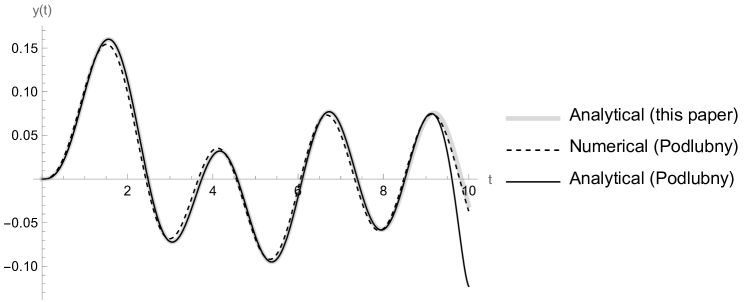
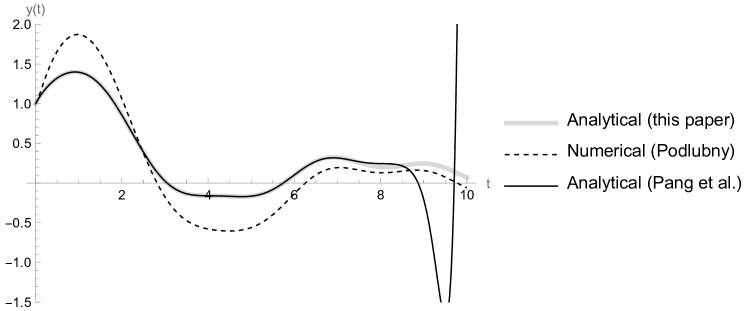
Figures 2-7 compare the solutions of the Bagley-Torvik equation (1) given in the literature with the solutions proposed in this paper, i.e. Theorem 6 for arbitrary $f\left(t\right)$, Theorem 8 for $f\left(t\right)=\sum_{\ell=0}^{n}C_{\ell}\,t^{\alpha_{\ell}}$, and Theorem 9 for $f\left(t\right)=\Omega\,\sin\omega\,t$. On the one hand, the analytical solutions found in the literature and computed in this section are given in (13)-(2.2), and (17)-(20). The stopping criterion for the recursive equation (19) of the latter method is that the series (18) is truncated when $\left|d_{k}\right|<10^{-12}$. On the other hand, the numerical solution found in the literature and computed in this section is described in Section 2, taking $200$ points within the interval $t\in\left(0,10\right)$.

Refer to caption
Figure 2: Solution of the Bagley-Torvik equation for a Bessel-type force with $y\left(0\right)=y^{\prime}\left(0\right)=0$.
Refer to caption
Figure 3: Solution of the Bagley-Torvik equation for a Bessel-type force with $y\left(0\right)=y^{\prime}\left(0\right)=1$.

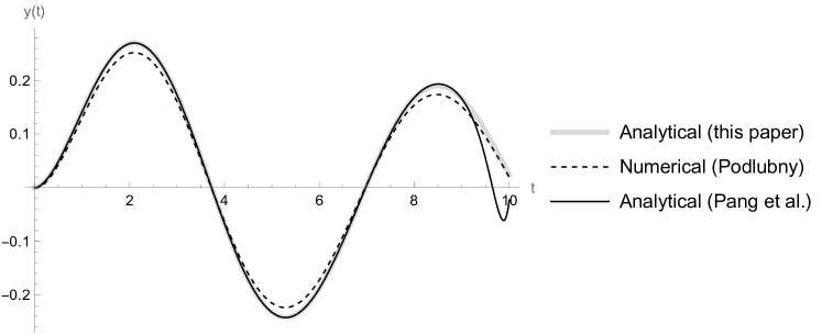
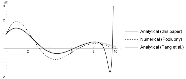
Figures 2 and 3 presents the solution of the Bagley-Torvik equation (1) with $f\left(t\right)=J_{0}\left(t\right)$, where $J_{0}\left(t\right)$ denotes the Bessel function of the first kind of zeroth order. Also, Figures 4 and 5 consider $f\left(t\right)=1+\sqrt{t}$, and Figures 6 and 7 takes $f\left(t\right)=\sin\omega t$ with $\omega=2.5$.

Refer to caption
Figure 4: Solution of the Bagley-Torvik equation for $f\left(t\right)=1+\sqrt{t}$ with $y\left(0\right)=y^{\prime}\left(0\right)=0$.
Refer to caption
Figure 5: Solution of the Bagley-Torvik equation for $f\left(t\right)=1+\sqrt{t}$ with $y\left(0\right)=y^{\prime}\left(0\right)=1$.

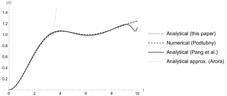
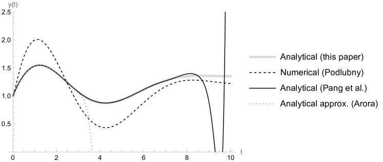
Figures 2, 4, and 6 consider homogeneous initial conditions, i.e. $y\left(0\right)=y^{\prime}\left(0\right)=0$; and Figures 3, 5 and 7, non-homogeneous initial conditions, i.e. $y\left(0\right)=y^{\prime}\left(0\right)=1$. Note that the performance of Podlubny’s numerical method is reasonably accurate when we have homogeneous initial conditions, but this is not the case when we have non-homogeneous initial conditions, where the accuracy is quite low. Also, Pang’s analytical solution is exactly the same as the one proposed in this paper, except for $t\gtrsim 9$, where the computation of (13)-(2.2) is not stable and starts to oscillate violently. Similarly, Arora’s analytical approximation is exactly the same as the one proposed here, but for $t\gtrsim 3$, the approximation of the truncated series (18) diverges from the actual solution.

Refer to caption
Figure 6: Solution of the Bagley-Torvik equation for a sinusoidal force with $y\left(0\right)=y^{\prime}\left(0\right)=0$.
Refer to caption
Figure 7: Solution of the Bagley-Torvik equation for a sinusoidal force with $y\left(0\right)=y^{\prime}\left(0\right)=1$.

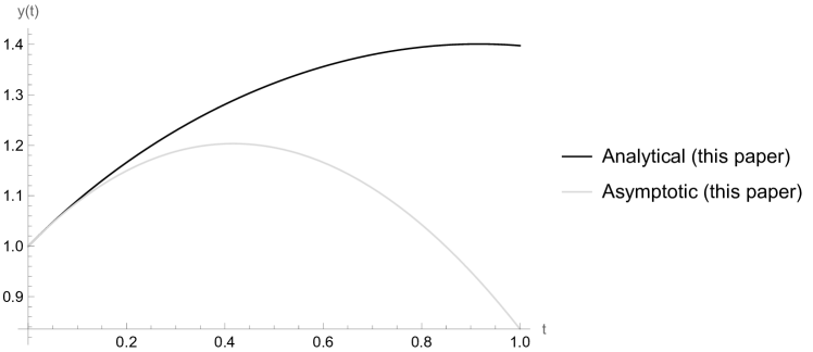
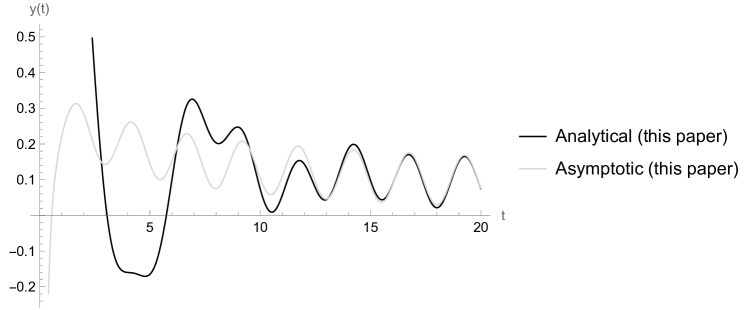
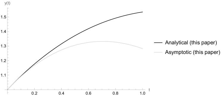
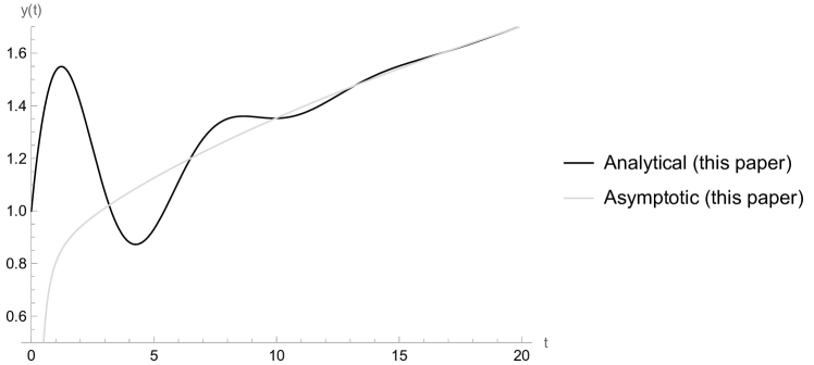
Figures 8 and 9 compares the sinusoidal solution, i.e. Theorem 9 for $f\left(t\right)=\sin\left(\omega t\right)$ with $\omega=2.5$, to its asymptotic behaviour as $t\rightarrow 0^{+}$, i.e. (92) and (99), and as $t\rightarrow+\infty$, i.e. (93) and (7.2), respectively. Likewise, Figures 10 and 11 compares the potential solution, i.e. Theorem 8 with $f\left(t\right)=1+\sqrt{t}$, to its asymptotic behaviour as $t\rightarrow 0^{+}$, i.e. (92) and (102), as well as $t\rightarrow+\infty$, i.e. (93) and (104), respectively. We have taken as initial conditions $y\left(0\right)=y^{\prime}\left(0\right)=1$ in all these figures.

Refer to caption
Figure 8: Asymptotic behaviour for $t\rightarrow 0^{+}$ of the Bagley-Torvik equation for a sinusoidal force with $y\left(0\right)=y^{\prime}\left(0\right)=1$.
Refer to caption
Figure 9: Asymptotic behaviour for $t\rightarrow+\infty$ of the Bagley-Torvik equation for a sinusoidal force with $y\left(0\right)=y^{\prime}\left(0\right)=1$.
Refer to caption
Figure 10: Asymptotic behaviour for $t\rightarrow 0^{+}$ of the Bagley-Torvik equation for $f\left(t\right)=1+\sqrt{t}$ with $y\left(0\right)=y^{\prime}\left(0\right)=1$.
Refer to caption
Figure 11: Asymptotic behaviour for $t\rightarrow+\infty$ of the Bagley-Torvik equation for $f\left(t\right)=1+\sqrt{t}$ with $y\left(0\right)=y^{\prime}\left(0\right)=1$.

9 Conclusions

We have calculated the solution $y\left(t\right)$ of the classical Bagley-Torvik equation (1) for arbitrary initial conditions $y\left(0\right)$, $y^{\prime}\left(0\right)$, and arbitrary external force $f\left(t\right)$ by applying the Laplace transform method, and calculating a new inverse Laplace transform. According to Theorem 6, this solution is the sum of two terms $y\left(t\right)=y_{f}\left(t\right)+y_{c}\left(t\right)$, where $y_{f}\left(t\right)$ takes into account the effect of $f\left(t\right)$, and $y_{c}\left(t\right)$ takes into account the effect of the initial conditions. The component $y_{c}\left(t\right)$ is a linear combination of exponentials with error functions. The component $y_{f}\left(t\right)$ is expressed in terms of a convolution integral of $f\left(t\right)$ and a linear combination of exponentials with error functions. The coefficients of these linear combinations for $y_{c}\left(t\right)$ and $y_{f}\left(t\right)$ are written in terms of the roots of a quartic equation, whose analytical expressions are given in (54) and (55). When $f\left(t\right)$ is a linear combination of potential or sinusoidal functions, the solution $y\left(t\right)$ can be expressed in closed-form, i.e. Theorems 8 and 9, respectively.

On the one hand, we have compared these solutions to other analytical solutions found in the literature, i.e. (13)-(2.2) and (17)-(20), and the agreement is excellent for moderate values of $t$. However, the computation of these analytical solutions found in the literature is increasingly complicated as $t$ increases, and at certain point the numerical accuracy is lost. This is not the case for the solutions given in Theorems 6, 8, and 9. Also, the numerical computation of the solution given in these theorems is much faster than the aforementioned analytical solutions found in the literature, above all in the cases of a sinusoidal or a potential external force.

On the other hand, we have compared the solutions given in Theorems 6, 8, and 9 with the numerical solution described in Section 2, and the agreement is quite good for homogeneous initial conditions, but is poor for non-homogeneous ones.

In addition, we have calculated the asymptotic behaviour of the solution as $t\rightarrow 0^{+}$ and as $t\rightarrow+\infty$. For the asymptotic behaviour of $y_{c}\left(t\right)$, we have used the version of the Tauberian theorem given in Theorem 10. In Section 8, we have numerically checked the asymptotic formulas obtained in Section 7.

All the computations and plots of this paper have been carried out with MATHEMATICA. The corresponding MATHEMATICA notebook is available at https://shorturl.at/i0SNN (accessed on November 2024).

Finally, we hope that the convolution integral given for $y_{f}\left(t\right)$ can be calculated for other types of external forces $f\left(t\right)$ as in the case of a sinusoidal force. Also, we expect that the analytical solution proposed in this paper can be used as a benchmark to test numerical schemes to solve other types of fractional differential equations.

Appendix A Auxiliary integrals

According to the definition of the Fresnel integrals [23, Eqns. 7.2.7-8]

$\displaystyle\mathrm{S}\left(z\right)$ $\displaystyle=$ $\displaystyle\int_{0}^{z}\sin\left(\frac{\pi t^{2}}{2}\right)dt,$ (112)
$\displaystyle\mathrm{C}\left(z\right)$ $\displaystyle=$ $\displaystyle\int_{0}^{z}\cos\left(\frac{\pi t^{2}}{2}\right)dt,$ (113)

and performing the change of variables $\frac{\pi t^{2}}{2}=\tau$, we obtain

$\displaystyle\mathrm{S}\left(\sqrt{\frac{2t}{\pi}}\right)$ $\displaystyle=$ $\displaystyle\frac{1}{\sqrt{2\pi}}\int_{0}^{t}\frac{\sin\tau}{\sqrt{\tau}}d\tau,$ (114)
$\displaystyle\mathrm{C}\left(\sqrt{\frac{2t}{\pi}}\right)$ $\displaystyle=$ $\displaystyle\frac{1}{\sqrt{2\pi}}\int_{0}^{t}\frac{\cos\tau}{\sqrt{\tau}}d\tau.$ (115)

Now, let us calculate the integral:

$\displaystyle\int_{0}^{t}\sin\left(t-\tau\right)\exp\left(r^{2}\tau\right)\,\mathrm{erfc}\left(-r\sqrt{\tau}\right)d\tau$
$\displaystyle=$ $\displaystyle\sin t\underset{I_{c}}{\underbrace{\int_{0}^{t}\cos\tau\exp\left(r^{2}\tau\right)\,\mathrm{erfc}\left(-r\sqrt{\tau}\right)d\tau}}-\cos t\underset{I_{s}}{\underbrace{\int_{0}^{t}\sin\tau\exp\left(r^{2}\tau\right)\,\mathrm{erfc}\left(-r\sqrt{\tau}\right)d\tau}}.$

Integrating by parts, and taking into account (114) and (115), we obtain

$\displaystyle I_{s}$ $\displaystyle=$ $\displaystyle\left.-\cos\tau\exp\left(r^{2}\tau\right)\,\mathrm{erfc}\left(-r\sqrt{\tau}\right)\right|_{0}^{t}+\frac{r}{\sqrt{\pi}}\int_{0}^{t}\frac{\cos\tau}{\sqrt{\tau}}d\tau$
$\displaystyle+r^{2}\int_{0}^{t}\cos\tau\exp\left(r^{2}\tau\right)\,\mathrm{erfc}\left(-r\sqrt{\tau}\right)d\tau$
$\displaystyle=$ $\displaystyle-\cos t\exp\left(r^{2}t\right)\,\mathrm{erfc}\left(-r\sqrt{t}\right)+1+\sqrt{2}r\ \mathrm{C}\left(\sqrt{\frac{2t}{\pi}}\right)$
$\displaystyle+r^{2}\left[\sin t\exp\left(r^{2}t\right)\,\mathrm{erfc}\left(-r\sqrt{t}\right)-\sqrt{2}r\ \mathrm{S}\left(\sqrt{\frac{2t}{\pi}}\right)-r^{2}I_{s}\right],$

thus

$$I_{s}=\frac{\exp\left(r^{2}t\right)\,\mathrm{erfc}\left(-r\sqrt{t}\right)\left(r^{2}\sin t-\cos t\right)+\sqrt{2}r\left[\mathrm{C}\left(\sqrt{\frac{2t}{\pi}}\right)-r^{2}\mathrm{S}\left(\sqrt{\frac{2t}{\pi}}\right)\right]+1}{1+r^{4}}.$$ (118)

Similarly, we arrive at

$$I_{c}=\frac{\exp\left(r^{2}t\right)\,\mathrm{erfc}\left(-r\sqrt{t}\right)\left(r^{2}\cos t+\sin t\right)-\sqrt{2}r\left[\mathrm{S}\left(\sqrt{\frac{2t}{\pi}}\right)+r^{2}\mathrm{C}\left(\sqrt{\frac{2t}{\pi}}\right)\right]-r^{2}}{1+r^{4}}$$ (119)

Insert (118) and (119) in (A), and simplify the result

$\displaystyle H_{r}\left(t\right)$
$\displaystyle=$ $\displaystyle\int_{0}^{t}\sin\left(t-\tau\right)\exp\left(r^{2}\tau\right)\,\mathrm{erfc}\left(-r\sqrt{\tau}\right)d\tau$
$\displaystyle=$ $\displaystyle\frac{1}{1+r^{4}}\left\{\exp\left(r^{2}t\right)\,\mathrm{erfc}\left(-r\sqrt{t}\right)-r^{2}\sin t-\cos t\right.$
$\displaystyle+\left.\sqrt{2}r\left[\mathrm{S}\left(\sqrt{\frac{2t}{\pi}}\right)\left(r^{2}\cos t-\sin t\right)-\mathrm{C}\left(\sqrt{\frac{2t}{\pi}}\right)\left(r^{2}\sin t+\cos t\right)\right]\right\}.$

Therefore, performing the change of variables $u=\omega\,\tau$, calculate the following integral as:

$\displaystyle\int_{0}^{t}\sin\omega\left(t-\tau\right)\exp\left(r^{2}\tau\right)\,\mathrm{erfc}\left(-r\sqrt{\tau}\right)d\tau$
$\displaystyle=$ $\displaystyle\frac{1}{\omega}\int_{0}^{\omega t}\sin\left(\omega t-u\right)\exp\left(\frac{r^{2}}{\omega}u\right)\,\mathrm{erfc}\left(-\frac{r}{\sqrt{\omega}}\sqrt{u}\right)du$
$\displaystyle=$ $\displaystyle\frac{1}{\omega}H_{r/\sqrt{\omega}}\left(\omega t\right)$
$\displaystyle=$ $\displaystyle\frac{1}{\omega^{2}+r^{4}}\left\{\omega\left[\exp\left(r^{2}t\right)\,\mathrm{erfc}\left(-r\sqrt{t}\right)-\cos\omega t\right]-\,r^{2}\sin\omega t\right.$
$\displaystyle+\left.\sqrt{\frac{2}{\omega}}r\left[\mathrm{S}\left(\sqrt{\frac{2\omega}{\pi}t}\right)\left(r^{2}\cos\omega t-\omega\sin\omega t\right)-\mathrm{C}\left(\sqrt{\frac{2\omega}{\pi}t}\right)\left(r^{2}\sin\omega t+\omega\cos\omega t\right)\right]\right\}.$

References

  • [1] Torvik, P., Bagley, R.: On the appearance of the fractional derivative in the behavior of real materials. J Appl Mech 51(2), 294–298 (1984)
  • [2] Podlubny, I.: Fractional Differential Equations: an Introduction to Fractional Derivatives, Fractional Differential Equations, to Methods of their Solution and some of their Applications. Academic Press (1999)
  • [3] Mainardi, F.: Fractional Calculus and Waves in Linear Viscoelasticity: an Introduction to Mathematical Models. World Scientific (2010)
  • [4] Zafar, A., Kudra, G., Awrejcewicz, J.: An investigation of fractional Bagley–Torvik equation. Entropy 22(1), 28 (2019)
  • [5] Basset, A.: The descent of a sphere in a viscous liquid. Nature 83(2122), 521–521 (1910)
  • [6] Mainardi, F., Pironi, P., Tampieri, F., Tabarrok, B., Dost, S.: On a generalization of the Basset problem via fractional calculus. Proceedings CANCAM 95(2), 836–837 (1995)
  • [7] Gorenflo, R., Kilbas, A., Mainardi, F., Rogosin, S.: Mittag-Leffler Functions, related Topics and Applications. Springer (2020)
  • [8] Oldham, K., Myland, J., Spanier, J.: An Atlas of Functions: with Equator, the Atlas Function Calculator. Springer (2009)
  • [9] Ray, S., Bera, R.: Analytical solution of the Bagley–Torvik equation by Adomian decomposition method. Appl Math Comput 168(1), 398–410 (2005)
  • [10] Diethelm, K., Ford, N.: Analysis of Fractional Differential Equations. J Math Anal Appl 265(2), 229–248 (2002)
  • [11] Pang, D., Jiang, W., Du, J., Niazi, A.: Analytical solution of the generalized Bagley–Torvik equation. Adv Differ Equ-NY 2019, 1–13 (2019)
  • [12] Arora, G., Pratiksha, P.: Solution of the Bagley–Torvik equation by fractional DTM. In: AIP Conf Proc, vol. 1860. AIP Publishing (2017)
  • [13] Lorenzo, C., Hartley, T.: Generalized Functions for the Fractional Calculus. NASA Centre for Aerospace Information (1999)
  • [14] Diethelm, K., Ford, J.: Numerical solution of the Bagley–Torvik equation. BIT 42, 490–507 (2002)
  • [15] De Bonis, M., Occorsio, D.: A global method for approximating Caputo fractional derivatives—an application to the Bagley–Torvik equation. Axioms 13(11), 750 (2024)
  • [16] Yüzbaşı, Ş.: Numerical solution of the Bagley–Torvik equation by the Bessel collocation method. Math Method Appl Sci 36(3), 300–312 (2013)
  • [17] Gülsu, M., Öztürk, Y., Anapali, A.: Numerical solution the fractional Bagley–Torvik equation arising in fluid mechanics. Int J Comput Math 94(1), 173–184 (2017)
  • [18] Schiff, J.: The Laplace Transform: Theory and Applications. Springer Science & Business Media (2013)
  • [19] González-Santander, J., Apelblat, A.: A note on some novel Laplace and Stieltjes transforms associated with the relaxation modulus of the Andrade model. Axioms 13(9), 647 (2024)
  • [20] Spiegel, M.: Mathematical Handbook of Formulas and Tables. McGraw-Hill (1968)
  • [21] González-Santander, J., Spada, G., Mainardi, F., Apelblat, A.: Calculation of the relaxation modulus in the Andrade model by using the Laplace transform. Fractal and Fractional 8(8), 439 (2024)
  • [22] Cohen, H., Rodriguez Villegas, F., Zagier, D.: Convergence acceleration of alternating series. Exp Math 9(1), 3–12 (2000)
  • [23] Olver, F., Lozier, D., Boisvert, R., Clark, C.: NIST Handbook of Mathematical Functions. Cambridge University Press (2010)