Expanding Molecular Shell and Possible $\gamma$-ray Source Associated with Supernova Remnant Kesteven 67

Abstract

We investigate the molecular environment of the supernova remnant  (SNR) Kesteven 67 (G18.8+0.3) using observations in ¹²CO, ¹³CO, HCO⁺, and HCN lines and possible associated $\gamma$-ray emission using 16-yr Fermi-LAT observation. We find that the SNR is closely surrounded by a molecular belt in the southeastern boundary, with the both recessed in the band-like molecular gas structure along the Galactic plane. The asymmetric molecular line profiles are widely present in the surrounding gas around local-standard-of-rest velocity $+20\,{\rm km}\,{\rm s}^{-1}$. The secondary components centered at $\sim+16\,{\rm km}\,{\rm s}^{-1}$ in the belt and $\sim+26\,{\rm km}\,{\rm s}^{-1}$ in the northern clump can be ascribed to the motion of a wind-blown molecular shell. This explanation is supported by the position-velocity diagram along a line cutting across the remnant, which shows an arc-like pattern, suggesting an expanding gas structure. With the simulation of chemical effects of shock propagation, the abundance ratios $N$(HCO⁺)/$N$(¹²CO) $\sim 2.6\times 10^{-5}$–$3.6\times 10^{-4}$ obtained in the belt can be more naturally interpreted by the wind-driven bubble shock than by the SNR shock. The belt and northern clump are very likely to be parts of an incomplete molecular shell of bubble driven by O-type progenitor star’s wind. The analysis of 0.2–500 GeV $\gamma$-ray emission uncovers a possible point source (‘Source A’) about 6.5$\sigma$ located in the north of the SNR, which essentially corresponds to northern molecular clump. Our spectral fit of the emission indicates that a hadronic origin is favored by the measured Galactic number ratio between CR electrons and protons $\sim 0.01$.

1 Introduction

Investigation of molecular environment of supernova remnants (SNRs) is of great importance in understanding the dynamical evolution of the SNR, hadronic $\gamma$-ray emission (Ackermann et al., 2013), ionizing low energy cosmic ray (CR) protons (Schuppan et al., 2014), the pre-supernova (SN) stellar wind (Chen et al., 2013), effects of shock chemistry (Draine & McKee, 1993), as well as the nearby triggered star formation (e.g. Cosentino & Shrec Collaboration, 2023).

In an SNR-molecular cloud (MC) association, it is very likely that a molecular gas bubble is blown inside the MC by the progenitor system of either core collapse or even Type Ia SN before the SN blastwave hits the MC or the molecular bubble shell (see e.g., Chen et al., 2013; Zhou et al., 2016; Sano et al., 2018). Therefore, the role of the wind-blown molecular bubble is unavoidable in studying the physical and chemical properties of the SNR. In this regard, Kes 67 is a typical object, in which the interplays of the progenitor’s bubble shell with both the ambient medium and SNR shock deserves deep examining.

SNR Kesteven 67 (G18.8+0.3; hereafter Kes 67 for short) has an unusual radio morphology, which is bright in the east and south and fades westward. At the southern edge, the radio emission displays a nearly right angle. The local-standard-of-rest (LSR) velocity center of this complex is at +19$\,{\rm km}\,{\rm s}^{-1}$ (Dubner et al., 1999; Paron et al., 2015) . The previous study of molecular environment of the remnant showed a positional agreement between the SNR shock and eastern elongated molecular feature. The far-infrared radiating dust was also detected around the SNR correlating with the molecular feature and supporting the shock-heated origin (Dubner et al., 1999). Paron et al. (2015) pointed out a coincidence between the indentations of the SNR radio continuum emission and the protrusions in the MC at the remnant’s southern boundary. These results strongly imply that the SNR shock have already interacted with MCs.

In addition to the MCs along the boundary of SNR, there are farther clumps to the east and south of the SNR, respectively. The eastern clump is suggested to be shaped by the HII region inside and have not been contacted by the shock front (Paron et al., 2012). The further southern molecular clumps, which are not corresponding to the position of ¹²CO peak, partially surround an HII region (Paron et al., 2015).

The Fe I K$\alpha$ line of 6.3-6.5 keV has been detected in Kes 67 (Nobukawa et al., 2018), indicating the penetration of low-energy CRs (LECRs) into the dense gas. This SNR is a soft X-ray source with an electron temperature of $\sim$0.4 keV (Nobukawa et al., 2018).

By means of CO emission and HI absorption features, the distance of Kes 67 has been constrained at the far-end from Earth and located at 13.8$\pm$0.4 kpc (Dubner et al., 2004; Tian et al., 2007; Ranasinghe & Leahy, 2018).

In this work, we study the molecular environment of Kes 67 using emission lines of molecular species ¹²CO, ¹³CO, HCO⁺, and HCN and search for $\gamma$-ray emission associated with the SNR. We present the spatial distribution and line profiles of the eastern molecular gas, calculate the column density ratio between HCO⁺ and CO, and use the Paris-Durham shock code to discuss the shock condition for the obtained abundance ratio. We analyse the 16 years of Fermi-LAT observation data and find $\gamma$-ray emission in energy range 0.2–500 GeV in the north of the remnant. The observation data are described in Section 2 and the analysis results are given in Section 3. The results are discussed in Section 4 and conclusions are in Section 5.

2 Observations and data

2.1 Millimeter Wave Molecular Line Data

We use the 13.7 m millimeter-wavelength telescope of the Purple Mountain Observatory at Delingha (hereafter PMOD), China, in 2020 June, to perform observation towards SNR Kes 67 in the HCO⁺ ($J$=1–0) line at $89.188\text{\,}\mathrm{G}\mathrm{H}\mathrm{z}$ and the HCN ($J$=1–0) line at $88.632\text{\,}\mathrm{G}\mathrm{H}\mathrm{z}$. The observation uses the on-the-fly (OTF) mapping mode. The half-power beam width (HPBW) is $\approx 60^{\prime\prime}$. We map a 22^′ $\times$22 ^′ area centred at (18${}^{\text{h}}$23${}^{\text{m}}$53${}^{\text{s}}$.83, $-$12^∘30^′11^′′.70, J2000.0), which includes most of the southern side of the remnant via raster-scan mapping with a grid spacing of 30^′′. We make the beam correction with the main-beam efficiency of 0.628. Using the GILDAS/CLASS package, the velocity resolution of both spectra was 0.25 km s^-1 and the $V_{\scriptscriptstyle\rm LSR}$ range was $-$100 km s^-1 to +150 km s^-1, and the pixel size was 30^′′. The RMS noise is $\sim$ 0.1 K for HCO⁺ and HCN.

We also use the archival data of the ¹²CO  ($J$=1–0) line at $115.271\text{\,}\mathrm{G}\mathrm{H}\mathrm{z}$ and the ¹³CO  ($J$=1–0) line at $110.201\text{\,}\mathrm{G}\mathrm{H}\mathrm{z}$ of the FOREST Unbiased Galactic plane Imaging survey with the Nobeyama 45 m telescope (FUGIN; Umemoto et al. (2017)) observation. The angular resolution was 20^′′ for ¹²CO and 21^′′ for ¹³CO . The average rms noise was $\sim$$1.5\text{\,}\mathrm{K}$ for ¹²CO and $\sim$$0.7\text{\,}\mathrm{K}$ for ¹³CO at a velocity resolution of 0.65 km s^-1.

2.2 Fermi-LAT $\gamma$-ray Data

For the $\gamma$-ray emission, we use about 16 yr observation data of Large Area Telescope (LAT) onboard the Fermi Gamma-ray Space Telescope. The time frame of our research is from 2008-08-04 15:43:36 (UTC) to 2024-07-21 02:17:41 (UTC), and the circular region of interest (ROI) is 15^∘ in radius, centred at the coordinates R.A.=275.96^∘, Dec=$-$12.4^∘ (J2000). We use the standard software Fermipy (Vertion 1.2.0 released on 2022 September 21), which bases on the Fermitools (Version 2.2.0 realesed on 2022 June 21) to analyze the data. We select ‘SOURCE’ class (evclass=128, evtype=3) with the instrument response function (IRF) ‘P8R3_SOURCE_V3_v1’ and constrain the energy range to 0.2-500 GeV. To eliminate the Earth’s limb, we limit the maximum of zenith to 90^∘. We also apply the recommended filter string ‘(DATA_QUAL¿0)&&(LAT_CONFIG==1)’ to choose the good time intervals. To build the background model, we use the Fermi-LAT Fourth Source Catalog Data Release 4 (Abdollahi et al. (2020), 4FGL-DR3 Abdollahi et al. (2022), 4FGL-DR4 Ballet et al. (2023)) in a radius of 15^∘ around the center of the ROI to consider the $\gamma$-ray sources, as well as the Galactic diffuse emission (gll_iem_v07.fits) and the isotropic emission (iso_P8R3_SOURCE_V3_v1.txt).

2.3 Other Data

We use the Multi-Array Galactic Plane Imaging Survey (MAGPIS) continuum image with angular resolution of 6^′′ at 1.4GHz (Helfand et al., 2006) to delineate the SNR boundary.

3 Data Analysis and Results

3.1 Millimeter-wavelength Molecular Lines

3.1.1 Molecular Gas Distribution

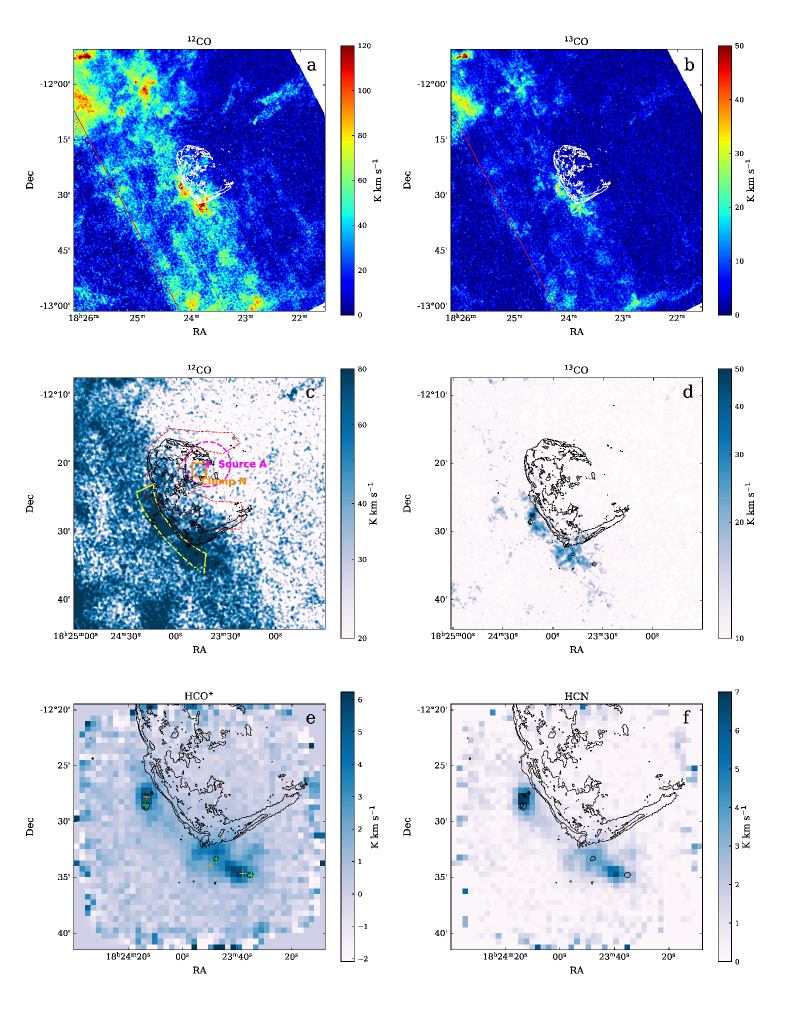
Figure 1: a, b): The integrated-intensity pseudo-color image of ¹²CO  ($J$=1–0) (left) and ¹³CO  ($J$=1–0) (right) in the $V_{\scriptscriptstyle\rm LSR}$ range from +10 km s^-1 to +30 km s^-1 in a large field of view, overlaid by the contours of 1.4 GHz radio continuum of 2, and 5 mJy beam^-1. The same contours are also plotted in other four panels c, d, e, f) in black. The solid red line masks the Galactic plane ($b=0$). c, d): The same as the top row, but in a small field of view and in greyscale. The orange box marks the position of Clump N. The magenta cross and dashed circle mark the position and 68% positional uncertainty of $\gamma$-ray source ‘Source A’ (see §3.2), and the dashed red polygon is the region of the enhanced Fe I K$\alpha$ line emission of Kes 67 adapted from Figure 1(b) in Nobukawa et al. (2018) .The dashed yellow lines surround the belt. e, f): Integrated-intensity maps of HCO⁺ and HCN from the PMOD observation in the $V_{\scriptscriptstyle\rm LSR}$ range in +10 – +30 km s^-1. The orange and green crosses represent ATLASGAL sources and HII regions, respectively.

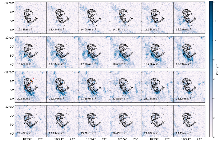
Figure 2: Velocity channel map of FUGIN ¹²CO  ($J$=1–0) emission on a scale of +12.8 km s^-1 to +27.7 km s^-1 with a step of 0.65 km s^-1, along with the contours of VLA 1.4GHz radio emission.

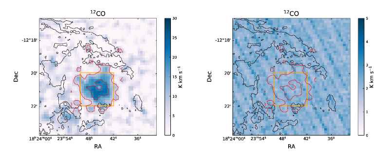
Figure 3: Integrated-intensity greyscale image of ¹²CO ($J$=1–0) of Clump N in the $V_{\scriptscriptstyle\rm LSR}$ range +20 – +22 km s^-1 (left panel) and 1 $\sigma$ level noise of integrated map (right panel), overlaid with the 1.4 GHz radio continuum contours of the SNR (in black) and the ¹²CO ($J$=1–0) contours of Clump N (in red). The orange box (the same as that in Figure 1c) marks the spatial range for extracting CO line spectra of Clump N.

The top row of Figure 1 shows that SNR Kes 67 is projected at the northwestern edge of a large band-like molecular gas structure, $\sim 25^{\prime}$ in thickness, above the Galactic plane ($b=0^{\circ}$), which is evident in the CO lines in the $V_{\scriptscriptstyle\rm LSR}$ range from +10 km s^-1to +30 km s^-1.

In the close-up CO maps (Figures 1c and 1d), the line emissions are bright in an outer belt closely along the southeastern edge of the remnant. There are two concentrations in the ‘belt’, one in the east and the other in the south. The two concentrations are also seen in the HCO⁺ and HCN maps with the same $V_{\scriptscriptstyle\rm LSR}$ range (Figures 1e and 1f). However, the brightness peaks of the eastern concentration is about $2^{\prime}$ from the eastern radio boundary. The eastern brightness peak appears to correspond to the eastern infrared clump that was discovered and suggested to contain proto-stars by Paron et al. (2012). The southern peak can be divided into two clumps, which are related to the HII regions G018.630+0.309 (R.A. = $18^{\text{h}}23^{\text{m}}47.8^{\text{s}}$, Dec = $-12^{\circ}33^{\prime}21^{\prime\prime}$) and G018.584+0.334 (R.A. = $18^{\text{h}}23^{\text{m}}34.9^{\text{s}}$, Dec = $-12^{\circ}34^{\prime}50^{\prime\prime}$) (Anderson et al., 2011) and also related to ATLASGAL sources AGAL018.626+00.297 (R.A. = $18^{\text{h}}23^{\text{m}}49.8^{\text{s}}$, Dec = $-12^{\circ}33^{\prime}53.8^{\prime\prime}$) and AGAL018.593+00.334 (R.A. = $18^{\text{h}}23^{\text{m}}38.0^{\text{s}}$, Dec = $-12^{\circ}34^{\prime}38.0^{\prime\prime}$) (Urquhart et al., 2014), respectively. The former HII region and ATLATGAL source have been noticed in Paron et al. (2015).

In Figure 2 we present the channel maps of ¹²CO  ($J$=1–0) in the velocity range from +12.78 km s^-1 to +27.73 km s^-1. In the range of +18 km s^-1 – +21 km s^-1, the molecular gas in the east and south in the field of view including the ‘belt’ has a sharp interface along the southeastern front of SNR shock wave represented by the radio contours. From +22 km s^-1 to +24 km s^-1, the southern molecular concentration appears to be coincident with the right-angle vertex of the radio boundary. A molecular clump (denoted as ‘Clump N’) can be discerned in the north of the SNR in the velocity range +20 km s^-1 – +22 km s^-1, which is also obvious in the ¹²CO integrated map (Figure 1c) and seems to be extended from the ‘belt’. Figure 3 shows the close-up towards Clump N presenting in ¹²CO ($J$=1–0) line, which is significant above 1 $\sigma$ level noise.

3.1.2 Molecular Line Profiles

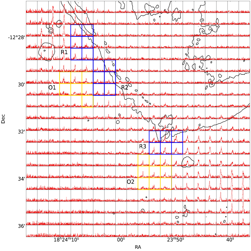
Figure 4: Grid map of HCO⁺ line profiles in the LSR velocity scale of 0 km s^-1 – +50 km s^-1 with the black contours of VLA 1.4GHz radio emission. The size of each pixel is 30^′′$\times$30^′′. Regions R1, R2 and R3 are marked with blue rectangles and regions O1 and O2 are marked with yellow rectangles, from which molecular line the spectra are extracted.

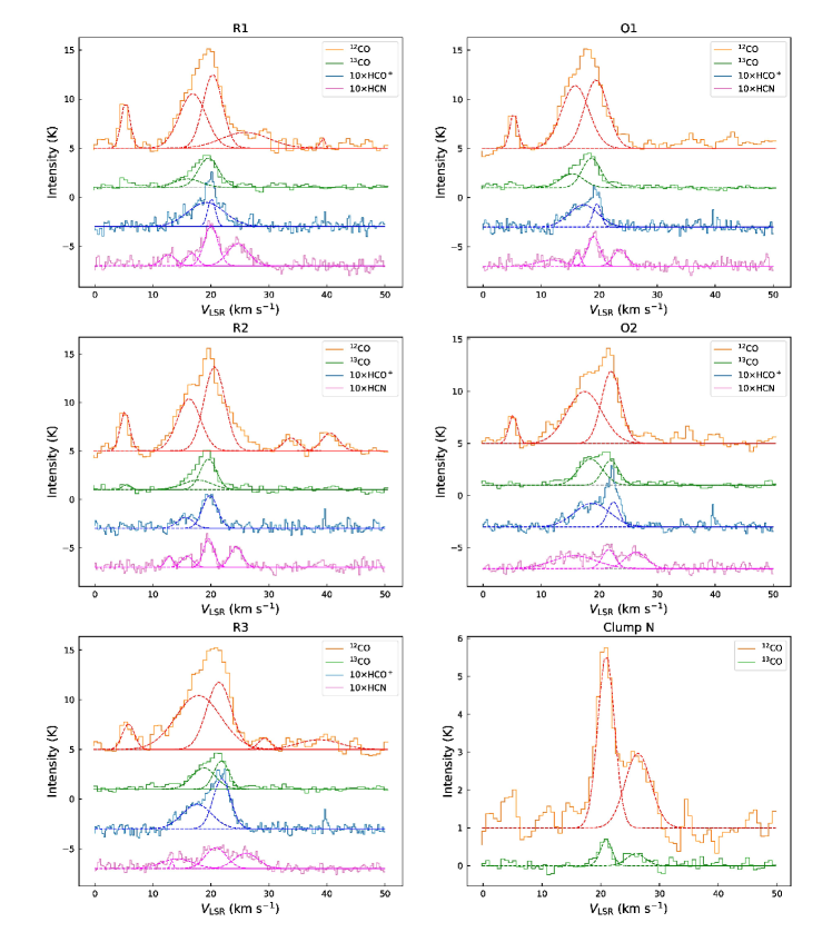
Figure 5: Averaged spectra and multi-Gaussian fitting results in velocity range from 0 km s^-1 to +50 km s^-1 for different molecular species. The intensity of HCO⁺ and HCN are multiplied by ten for comparison.

Table 1: Multi-Gaussian fitting results and column densities for the secondary components of molecular lines as shown in Figure 5.

Region	Molecule	$v_{0}$ / km s-1	$T_{\rm peak}$ / K	FWHM / km s-1	Integration / K  km s-1	$N$(species) / cm-2
	12CO	16.86$\pm$1.28	5.07$\pm$ 2.18	3.35$\pm$0.50	24.30 $\pm$ 13.97	2.20 $\pm$ 0.80 $\times 10^{16}$
R1	13CO	15.97$\pm$1.84	0.85$\pm$0.15	3.57$\pm$1.3	4.91 $\pm$ 1.14	4.69 $\pm 1.09\times 10^{15}$
	HCO+	19.18$\pm$0.20	0.24$\pm$0.03	4.19$\pm$1.08	1.94 $\pm$ 0.43	7.85 $\pm 1.50\times 10^{12}$
	HCN	16.73$\pm$0.27	0.13$\pm$0.02	2.35$\pm$0.35	0.75 $\pm$ 0.13	1.73 $\pm 0.73\times 10^{12}$
	12CO	16.46$\pm$0.69	5.98$\pm$1.15	3.33$\pm$0.71	21.07 $\pm$ 7.22	5.06 $\pm 2.04\times 10^{17}$
R2	13CO	17.72$\pm$1.92	1.00$\pm$0.43	3.72$\pm$1.82	6.15 $\pm$ 2.31	5.92 $\pm 2.23\times 10^{15}$
	HCO+	15.91$\pm$0.2	0.11$\pm$0.02	2.78$\pm$0.35	0.40 $\pm$ 0.17	1.31 $\pm 0.55\times 10^{12}$
	HCN	15.90$\pm$0.19	0.11$\pm$0.02	2.35$\pm$0.28	0.27 $\pm$ 0.09	1.70 $\pm 0.55\times 10^{12}$
	12CO	17.88$\pm$1.63	5.26$\pm$1.56	4.63$\pm$1.82	52.61 $\pm$ 19.69	8.56 $\pm 4.58\times 10^{16}$
R3	13CO	18.76$\pm$0.88	2.16$\pm$0.35	3.33$\pm$1.33	10.83 $\pm$ 3.25	1.03 $\pm 0.30\times 10^{16}$
	HCO+	17.60$\pm$0.54	0.25$\pm$0.02	3.73$\pm$0.28	1.57 $\pm$ 0.32	5.12 $\pm 1.06\times 10^{12}$
	HCN		(undistinguishable)
	12CO	15.86$\pm$2.75	6.42$\pm$1.04	3.65$\pm$0.82	31.82 $\pm$ 22.19	6.43 $\pm 4.2\times 10^{16}$
O1	13CO	15.30$\pm$1.58	1.43$\pm$0.55	3.33$\pm$1.05	7.17 $\pm$ 3.21	6.96 $\pm 2.48\times 10^{15}$
	HCO+	17.29$\pm$0.28	0.024$\pm$0.03	3.71$\pm$0.14	1.41 $\pm$ 0.20	4.59 $\pm 0.64\times 10^{12}$
	HCN		(undistinguishable)
	12CO	17.57 $\pm$0.97	5.67$\pm$0.57	4.08$\pm$1.45	37.60 $\pm$ 12.53	7.04 $\pm 2.72\times 10^{16}$
O2	13CO	18.50$\pm$ 0.58	2.53$\pm$0.23	3.63$\pm$1.29	12.94 $\pm$ 3.2	1.23 $\pm 0.3\times 10^{16}$
	HCO+	18.78$\pm$0.39	0.22$\pm$0.01	4.10$\pm$0.19	1.65 $\pm$ 0.21	5.37 $\pm 0.77\times 10^{12}$
	HCN		(undistinguishable)
	12CO	25.99$\pm$0.35	1.98$\pm$0.16	3.35$\pm$1.05	10.90 $\pm$ 2.34	1.14 $\pm 0.26\times 10^{16}$
Clump N	13CO	26.04$\pm$ 0.34	0.32$\pm$0.06	2.98$\pm$1.02	1.30 $\pm$ 0.48	1.46 $\pm 0.56\times 10^{15}$

• Note——$v_{0}$ denotes the center velocity of the secondary components. $N$ in the 7th columns denotes the column density of the specific molecular species.

Table 2: Calculated parameters for the secondary components of molecular lines as shown in Figure 5.

Region	$N$(HCO+)/$N$(CO)	$M$ /$M_{\odot}$	$n({\rm H}_{2})$ / cm-3
R1	3.6 $\pm 1.6\times 10^{-4}$	1800	300
R2	2.6 $\pm 1.5\times 10^{-5}$	2200	320
R3	6.0 $\pm 3.4\times 10^{-5}$	3900	600
O1	7.0 $\pm 4.6\times 10^{-5}$	1700	400
O2	8.0 $\pm 3.1\times 10^{-5}$	7000	500
Clump N	- - -	1500	40

Figure 4 is a grid map of HCO⁺ line spectra at $V_{\scriptscriptstyle\rm LSR}$ between $0\,{\rm km}\,{\rm s}^{-1}$ and $+50\,{\rm km}\,{\rm s}^{-1}$. Inside the radio boundary of the SNR, there is little line features; by contrast, evident line features are present outside the boundary, also illustrating that there is a sharp interface between the SNR and the outer molecular gas. Notably, in the outer region, the line features around $\sim+20\,{\rm km}\,{\rm s}^{-1}$ are asymmetric, extending from $\sim+10\,{\rm km}\,{\rm s}^{-1}$ to $\sim+25\,{\rm km}\,{\rm s}^{-1}$.

Specifically, as shown in Figure 4, we select three on-boundary regions, R1, R2, and R3, along the southeastern border of the remnant and two outer regions, O1 and O2, for the use of extraction of molecular line spectra around the SNR. The five selected regions do not overlap with the HII regions discussed in Paron et al. (2012); Paron et al. (2015). The data of the CO lines and the data of the HCO⁺ and HCN lines come from different telescopes; for uniform format, the CO data have been regridded to the coordinate and spatial resolution of the HCO⁺ and HCN data when extracting the molecular spectra.

Figure 5 shows the averaged emission line spectra of the four molecular species HCO⁺, HCN, ¹²CO, and ¹³CO extracted from the five selected regions. The line spectra of Clump N are extracted from the region marked in Figure 3. In the spectra of the three regions along the SNR boundary (R1, R2, and R3), we see small component of ¹²CO at $\sim$+5 km s^-1 that corresponds to the local gas emission (Paron et al., 2012). For all of the four molecular species in regions R1, R2, and R3, main components appear around $+20$ km s^-1 with a secondary component from $\sim$+10 km s^-1 to $\sim$+18 km s^-1. The Gaussian fitting results of the secondary components are given in Table 1. The secondary components could represent the blue-shifted broadened line wings as a signature of disturbance of the molecular gas by passing shock waves (e.g., Jiang et al., 2010). However, in Figure 4, the grid map of HCO⁺ shows that similar line profiles are also seen in the outer regions O1 and O2, which indicates that the secondary components in the line profiles do not appear only along the southeastern boundary of the SNR.

Furthermore, the line profiles of HCN comprise at least three components in the range of $\sim$ +10 km s^-1 to $\sim$+30 km s^-1 (see Figure 5). The HCN rotational levels include hyperfine structure (HFS) and have three components. Each hyperfine level is designated by a quantum number $F$ (= $I$ + $J$) and the strengths of the HCN ($J$=1–0) HFS lines is 1:5:3 in the optical thin limit. Theoretically, the LSR velocity difference between the $F=\,0$ – 1 line and $F=\,2$ – 1 line is $-$7.1 km s^-1, and that between the $F=\,1$ – 1 line and $F=\,2$ – 1 line is 4.9 km s^-1 (Goicoechea et al., 2022). In Figure 6, we show the fitting result taking the HCN spectrum of region R2 as an example, which includes four components: those fitted in red are related to HFS and that fitted in cyan is related to a secondary or broadened component. The $F=\,2$ – 1, $F=\,0$ – 1, and $F=\,1$ – 1 lines are centered at +19.63 km s^-1, +12.79 km s^-1, and +24.35 km s^-1, respectively. The separation between the $F=\,0$ – 1 and $F=\,2$ – 1 lines is $-$6.84 km s^-1, and that between the $F=\,1$ – 1 and $F=\,2$ – 1 is 4.72 km s^-1. Although the measured separations are slightly different from the theoretical values, the HFS of the HCN molecules can be identified because the differences are similar to or less than the velocity resolution (0.25$\,{\rm km}\,{\rm s}^{-1}$). The secondary or broadened component of HCN is centered at 15.90 km s^-1, which could be of the same origin as the secondary or broadened components of ¹²CO and HCO⁺ in region R2.

For Clump N, we extract the averaged spectrum of two components of the line profiles, also shown in Figure 5. Besides the main component of ¹²CO in $V_{\scriptscriptstyle\rm LSR}$ range $\sim+18\,{\rm km}\,{\rm s}^{-1}$ – $\sim+24\,{\rm km}\,{\rm s}^{-1}$, there is also a secondary component in $V_{\scriptscriptstyle\rm LSR}$ range $\sim+24\,{\rm km}\,{\rm s}^{-1}$ – $\sim+30\,{\rm km}\,{\rm s}^{-1}$. The Gaussian fitting results for Clump N are also listed in Table 1.

We produce a position-velocity (P-V) diagram Figure 7 along the red line from region R2 to Clump N marked in Figure 2. Figure 7 shows an arc-like distribution pattern, which indicates a $V_{\scriptscriptstyle\rm LSR}$ span from $\sim+14\,{\rm km}\,{\rm s}^{-1}$ to $\sim+26\,{\rm km}\,{\rm s}^{-1}$. Such a pattern suggests an expanding gas structure centered at $V_{\scriptscriptstyle\rm LSR}\sim+20\,{\rm km}\,{\rm s}^{-1}$.

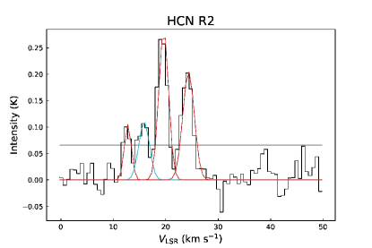
Figure 6: The line profiles of HCN in region R2, with 3 $\sigma$ line in black. The red components show the fitting results of HFS with the $F$=1-0 line, which centered at $\sim$19.63 km s^-1. The component of HCN fitted in cyan coincides with the secondary component of HCO⁺ in region R2 and is not related to the HFS lines. The velocity resolution has been rebinned to 0.65$\,{\rm km}\,{\rm s}^{-1}$ for better displaying effect.

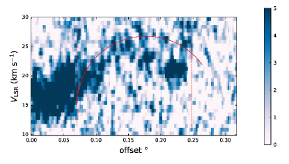
Figure 7: The position-velocity diagram extracted along the path (marked in red in Figure 2) from region R2 to Clump N. The red vertical dashed lines delineate the position of region R2 and Clump N (marked by the orange diamonds in Figure 2). The red arc indicates a general P-V pattern.

3.1.3 Parameters of Molecular Gas

Using the local thermodynamic equilibrium (LTE) hypothesis, we calculate the column densities of ¹²CO, ¹³CO, HCO⁺, and HCN molecules in the secondary or broadened components for the molecualar gas in the five selected regions and Clump N and list the results in Table 1. Here we have assumed the ¹²CO line is optically thick while the other lines of ¹³CO, HCO⁺, and HCN are optically thin, and thus the column densities for the optically thick and thin cases are given by (Mangum & Shirley, 2015):

$$N_{\rm thick} =\frac{3h}{8\pi^{3}\mu^{2}J_{\mu}R_{\rm i}}\left(\frac{kT_{\rm ex}}{hB_{\rm 0}}+\frac{1}{3}\right)\frac{\exp{(E_{\rm u}/kT_{\rm ex}})}{\exp{(E_{\rm u}/kT_{\rm ex})}-1}$$ (1)

$$\times\int-\ln{\left[1-\frac{T_{\rm R}}{J_{\nu}\left(T_{\rm ex}\right)-J_{\nu}(T_{\rm bg})}\right]}dv$$

and

$$N_{\rm thin} =\frac{3h}{8\pi^{3}\mu^{2}J_{\mu}R_{\rm i}}\left(\frac{kT_{\rm ex}}{hB_{\rm 0}}+\frac{1}{3}\right)\exp{\frac{E_{\rm u}}{kT_{\rm ex}}}$$ (2)

$$\times\left(\exp{\frac{h\nu}{kT_{\rm ex}}}-1\right)^{-1}\int\tau_{\rm\nu}dv,$$

respectively, where $J\left(T\right)=h\nu/[\exp{(h\nu/kT)}-1]$, and $T_{\rm bg}$ is the cosmic microwave background temperature (also see Mangum & Shirley (2015) for definition of other symbols in the above equations). The optical thin assumption for HCO⁺ may underestimate the column density.

The excitation temperature of ¹²CO is estimated using (Mangum & Shirley, 2015)

$$T_{\rm ex} =\frac{h\nu/k_{\rm B}}{\ln{\left[1+\frac{h\nu/k_{\rm B}}{T_{\rm max}+J_{\rm\nu}(T_{\rm cmb)}}\right]}}\sim 14\,{\rm K},$$ (3)

where $k_{\rm B}$ is the Boltzmann constant, and $T_{\rm max}$ is the maximum brightness temperature taken from the molecular lines. Then, we calculate the column density ratios $N$(HCO⁺)/$N$(¹²CO), which are listed in Table 2. We obtain the column densities of hydrogen molecules from $N({\rm{}^{13}CO})$ (as listed in Table 1) using abundance ratio $N({\rm H_{2}})/N({\rm{}^{13}CO})\approx 7\times 10^{5}$ (Frerking et al., 1982). On the assumption that the line-of-sight depth in each region is similar to the transverse size, we estimate the mass of the secondary component by $M=2.8m_{\rm H}N({\rm H}_{\rm 2}){\cal A}$ (where ${\cal A}$ is the projected area for each region from which the molecular line spectra are extracted (see Figure 3 and Figure 4)) and number density $n({\rm H}_{2})$. The mass and number density values are listed in Table 2. The lower limit of the mass of the secondary component in the molecular belt is estimated by summing the masses of the secondary components in the five selected regions. The upper limit is estimated by multiplying the average column density of the five regions by the projected size of the belt. The estimated mass ranges from $\sim 1.6\times 10^{4}$ to $\sim 4.7\times 10^{4}M_{\odot}$, and we will use the average $\sim 3.1\times 10^{4}M_{\odot}$ in later calculations.

3.2 Fermi-LAT Data Analysis

3.2.1 Spatial Analysis

We use the 4FGL-DR4 catalogue in our $\gamma$-ray data analysis and there are no catalogue sources in the field of view around SNR Kes 67. When fitting the models, we free the spectral parameters of sources within 5^∘ ROI above 5$\sigma$ and the normalization of the Galactic and isotropic diffuse background. Then we fix all parameters except the normalization parameters of the Galactic and isotropic diffusion background component and generate the residual test-statistic (TS) map of the 1.5^∘$\times$1.5^∘ region centered at the SNR. The test statistic is defined as TS$=2\log{\left({\cal L}_{1}/{\cal L}_{0}\right)}$, in which ${\cal L}_{0}$ is the maximum likelihood of the null hypothesis and ${\cal L}_{1}$ is the maximum likelihood with a putative source located in the tested pixel. The TS map is shown in Figure 8. As seen in Figure 8a, there is residual $\gamma$-ray emission in the north of the SNR.

We select photon events above 1 GeV for spatial analysis to reduce uncertainties. We add a source with a single power-law (PL) spectrum into the background model at the pixel of the maximum TS value, which is denoted as ‘Source A’. With the extension method in Fermipy, we do not detect any extension for ‘Source A’, so we still use the point source (PS) model for further analysis. Using the source  localization method in Fermipy, we obtain the best fitted position of ‘Source A’ , which is (R.A.=$275.9203^{\circ}$, Dec.=$-12.3349^{\circ}$, J2000), with the 95% positional uncertainty is 0.059^∘, as illustrated in Figure 8 (and also marked in Figure 1c). This point source could explain the emission near the SNR and there is still residual emission in the region. We add another point sources (‘P1’), as listed in Table 3 with a single PL spectrum to the background template. Then we test the two point sources template in the energy range of 0.2–500 GeV. The final residual map is shown in the right panel of Figure 8 in 0.2–500 GeV, there is almost no residual $\gamma$-ray emission with the two additive sources.

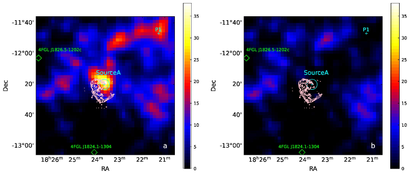
Figure 8: TS maps of 1.5^∘$\times$1.5^∘ field covering SNR Kes 67 in the energy range of 0.2–500 GeV. The image scale of the TS maps is 0.05^∘ per pixel. The radio contours are the same as those in Figure 1

. The cyan circle marks the best fitted location of ‘Source A’ and the range of 95% positional uncertainty. Left: TS map without source points designated. Right: residual TS map after adding the point source ‘Source A’ and source ‘P1’.

Table 3: Coordinates for two sources in energy range of 0.2–500 GeV

Name	R.A.(J2000)	Dec.(J2000)	TS
SourceA	275.9203	$-$12.3349	52.83
P1	275.3207	$-$11.7820	26.64

3.2.2 Spectral Analysis

With the PS spatial model for ‘Source A’, we select photon events in the energy range of 0.2–500 GeV for $\gamma$-ray spectral analysis. In the spectral analysis, we also take into account three other spectral models: log-parabola (LP), exponentially cutoff power-law (ECPL), and broken power-law (BPL) in addition to the PL model. The formulae of these spectral models are listed in Table 4. To determine the best fitted model, we define the TS_spec = 2$\log{\left(\mathcal{L}_{\rm spec}/\mathcal{L}_{\rm PL}\right)}$and choose the model with the largest TS_spec value. The test results are listed in Table 5, and thus we choose the PL model.

Table 4: Formulae for $\gamma$-ray spectra

Name	Formula	Free Parameters
PL	$dN/dE=N_{0}\left(E/E_{0}\right)^{-\Gamma}$	$N_{0},\Gamma$
ECPL	$dN/dE=N_{0}\left(E/E_{0}\right)^{-\Gamma}\exp{\left(-E/E_{\rm cut}\right)}$	$N_{0},\Gamma,E_{\rm cut}$
LogP	$dN/dE=N_{0}\left(E/E_{0}\right)^{-\Gamma-\beta\log{\left(E/E_{0}\right)}}$	$N_{0},\Gamma,\beta$
BPL	$dN/dE=N_{0}\begin{cases}\left(E/E_{\rm b}\right)^{-\Gamma_{1}}&\text{$E\leq E_{\rm b}$}\\ \left(E/E_{\rm b}\right)^{-\Gamma_{2}}&\text{$E\geq E_{\rm b}$}\end{cases}$	$N_{0},E_{\rm b},\Gamma_{1},\Gamma_{2}$

Table 5: Test results of spectral models for ‘Source A’

Spectral Model	TSspec
PL	0
ECPL	$-$1.03
LogP	$-$1.03
BPL	$\sim$-1.5\text{\times}{10}^{6}$$

Fermipy gives the TS value of ‘Source A’ is 52.83 with the PS spatial model and the PL spectral model, which is 6.5$\sigma$. We obtain the 0.2–500 GeV $\gamma$-ray flux $\sim$9.6\text{\times}{10}^{-12}$\,{\rm erg}\,{\rm cm}^{-2}\,{\rm s}^{-1}$ and the index $\Gamma=2.35\pm 0.11$, which leads to the luminosity $\sim 1.78\times 10^{34}{\rm erg}\,{\rm s}^{-1}$ at a distance of $d\sim$14 kpc.

Using the SED method of Fermipy, the spectral energy distribution (SED) of ‘Source A’ in the energy range of 0.2–500 GeV is generated by using the maximum likelihood analysis in five logarithmically spaced energy bins. In the fitting process, we free the normalization parameters of the sources within 3^∘ from the ROI center and the Galactic and isotropic diffuse background parameters. In the energy bins, when the TS value of ‘Source A’ is less than 4, we calculate the 95% confidence level upper limit of flux. The SED results are shown in Figure 9. For further restriction, we use the radio flux data presented in the previous literature (listed in Table 6) of the entire SNR.

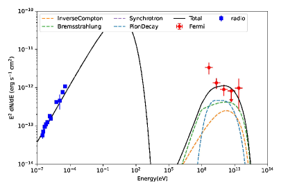
Figure 9: The SED of ‘Source A’. The radio data are listed in Table 6.

4 Discussion

4.1 The SNR-MC Association

As revealed in our spatial analysis of the molecular environment of SNR Kes 67, the molecular belt that closely surrounds the southeastern boundary of the SNR is recessed in the band-like molecular gas structure (§3.1.1). The molecular belt looks like a cushion between the SNR and the molecular band. This is a perfect morphological evidence for the physical contact among the SNR, the belt, and the band. Actually, the elongated structure (named ‘feature A’) discerned by Dubner et al. (1999) in a much lower spatial resolution seems similar to the belt our study shows and was suggested as the indication of SNR-MC physical association. Figure 1 in Paron et al. (2012) for ¹³CO ($J$=1–0) emission with similar angular resolution also presents a comparable belt-like morphology.

4.1.1 The asymmetric broad line profiles

The SNR-MC association is supported by the asymmetric molecular line profiles that we obtain (§3.1.2), which could be caused by the perturbation from SNR shock or progenitor’s wind. The secondary components at $\sim+16\,{\rm km}\,{\rm s}^{-1}$ of the four molecular species in the five regions in the belt (see Table 1) could result from the perturbation that the molecular gas suffers. If the perturbation come from the SNR shock, the asymmetric broad line profiles in the positions on the SNR shock front (such as regions R1, R2, and R3) could be explained. However, the line profiles in the positions away from the SNR shock front (such as regions O1 and O2) are very similar to those in regions R1, R2, and R3, and cannot be ascribed to SNR shock impact. Notwithstanding, the asymmetric broad line profiles in the molecular belt can be explained if the source of perturbation is the wind of the SNR’s progenitor star, which could drive a wind shock into the band-like structure. In the latter case, the belt may be a segment of shell swept up by the wind. This segment, with a mass $\sim 3.1\times 10^{4}M_{\odot}$ was deposited a kinetic energy $\sim 1\times 10^{49}\,(v_{\rm b}/6\,{\rm km}\,{\rm s}^{-1})^{2}\,{\rm erg}$ (with $v_{\rm b}$ the velocity of the shell motion) from the wind before the impact by the supernova blast wave.

Also, from the view angle of shock chemistry, the HCN-to-HCO⁺ and HCO⁺-to-¹²CO abundance ratios seem more consistent with the scenario of the molecular belt’s perturbation by the progenitor’s wind than that by the SNR shock, as discussed below.

Moreover, for Clump N in the north, the secondary component around $\sim+26\,{\rm km}\,{\rm s}^{-1}$ can be ascribed to a red-shifted broadening from the main component around $\sim+20\,{\rm km}\,{\rm s}^{-1}$. It is consistent with a patch of backward moving molecular gas also driven by the progenitor’s wind.

Furthermore, the blue-shift in the molecular line wings in the belt and the red-shift in Clump N are consistent with the expanding motion at velocity $\sim 6\,{\rm km}\,{\rm s}^{-1}$ that is uncovered by the P-V diagram (Figure 7), which can be compatible with the case of wind-driven shell.

4.1.2 The molecular abundance ratios

The abundance ratio $N$(HCO⁺)/$N$(¹²CO) in the five regions is in a range from $7.2\times 10^{-5}$ to $4.0\times 10^{-4}$. Similarly, we use the secondary or broadened components in region R2 (shown in Figure 5 and Figure 6 ) to estimate the abundance ratio $N({\rm HCN})/N({\rm HCO}^{+})$ in the region and obtain a value $\sim 1.2$. This ratio value is very similar to the $N({\rm HCN})/N({\rm HCO}^{+})$ ratio, $1.9\pm 0.9$, which is obtained in the diffuse interstellar medium (Godard et al., 2010). However, the ratio is not much different from those obtained in SNR IC 433. The ratios obtained in IC 433 are model dependent, ranging from 2.7 to 30 (van Dishoeck et al., 1993). The HCN-to-HCO⁺ ratios can also be much lower in SNRs; for example, the ratio is $\sim 0.4$ for the MC interacting with SNR G349.7+0.2 (Lazendic et al., 2010).

For the possibility of shock-induced asymmetry in molecular line profiles, the column density ratio $N({\rm HCO}^{+})/N({\rm{}^{12}CO})$ may reflect the chemical effect of the shock in two cases. The first case is that a preshock gas like that in the belt with a density $\sim 10^{3}\,{\rm cm}^{-3}$ is traversed by the shock driven by the SNR at a velocity 10 – $50\,{\rm km}\,{\rm s}^{-1}$ for a timescale $\sim 20$ kyr. This case is assumed for the emission from regions R1, R2, and R3. Actually, the beam size of the PMOD observation of HCO⁺ and HCN is $\sim 1^{\prime}$, the emission from R1, R2, and R3 may contain the contribution from the molecular gas disturbed by the SNR shock (if any). For LECRs , the cross section of ionization can be estimated by $4\pi a_{0}^{2}[0.71\ln{(1+m_{\rm e}E_{\rm p}/m_{\rm p}I({\rm H}))}+1.63]/(m_{\rm e}E_{\rm p}/m_{\rm p}I({\rm H}))$, in which $I({\rm H})=13.6$ eV, $a_{0}=0.539$ Å  (Padovani et al., 2009; Bloemen, 1989). The cross section values of 10 MeV and 100 MeV CR protons are $\sim 3.8\times 10^{-18}$ and $\sim 6.8\times 10^{-19}$ cm^-2, respectively, corresponding to the mean free path values of protons $\sim 1.3\times 10^{14}$ and $7.3\times 10^{14}$ $(n({\rm H}_{2})/2000\,{\rm cm}^{-3})^{-1}\,{\rm cm}$, much less than 1 pc. Therefore, the accelerated CR particles cannot pass through the molecular belt to arrive at the outer regions O1 and O2.

The second case is that a preshock molecular gas with a density $\sim 10^{2}\,{\rm cm}^{-3}$ is swept up by the wind-driven shock having evolved to the steady state. This case is assumed for all the five regions in the molecular belt that is considered as a segment of wind-swept shell.

We apply the Paris-Durham shock model to examine the chemistry evolution on the path of shock propagation in these two cases (Flower & Pineau des Forêts, 2003; Godard et al., 2019). The Paris-Durham chemistry network contains 140 molecular species and over 3000 chemical reactions, including HCO⁺ and CO. Here, the HCO⁺-to-¹²CO abundance ratio is calculated for a range of velocity, $v_{\rm c}$, of shock propagation in the MC for each case. In the model calculation, the magnetic field strength in the cloud is taken as $B\approx\sqrt{n({\rm H}_{2})/\,{\rm cm}^{-3}}\,\mu\mbox{G}$. In addition, we take into account the molecular ionisation induced by low-energy ($<280$ MeV) CRs. Two CR ionization rates are adopted: $\zeta=$2.6\text{\times}{10}^{-17}$\,{\rm s}^{-1}$ typical of Galactic value (van der Tak & van Dishoeck, 2000) and $\zeta=$2.6\text{\times}{10}^{-15}$\,{\rm s}^{-1}$ for the gas ionized by SNR-accelerated CRs (e.g., Ceccarelli et al., 2011; Vaupré et al., 2014; Zhou et al., 2022; Tu et al., 2024b). The calculation results are shown in Figure 10.

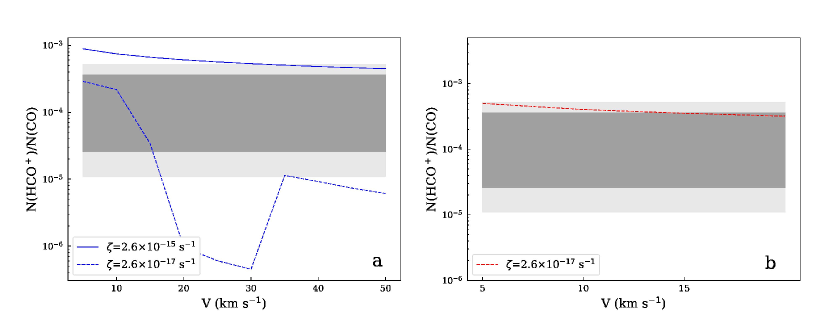
Figure 10: HCO⁺-to-¹²CO abundance ratio calculated using the Paris-Durham shock model, in comparison with the abundance ratio ranges (in dark grey) obtained from observations with the best-fitted parameters listed in Table 2 and the uncertainty ranges (in light grey). The used CR ionization rates ($\zeta$) are marked in the panels. a) The ratio for a high-density ($10^{3}\,{\rm cm}^{-3}$) molecular gas. b) Same as in a), but for lower-density ($10^{2}\,{\rm cm}^{-2}$) molecular gas.

For the first case assumed for SNR shock (Figure 10a), the calculated abundance ratios for the five regions for $\zeta=2.6\times 10^{-15}\,{\rm s}^{-1}$ is slightly above the range of observed values, but still within the uncertainty range. Thus the chemical effects of the SNR shock together with CRs cannot be excluded. For $\zeta=2.6\times 10^{-17}\,{\rm s}^{-1}$, which represents that the ionizing CRs from the SNR are not at work, the calculated ratios can match the observational values at $v_{\rm c}$ around $10\,{\rm km}\,{\rm s}^{-1}$ for a C-type shock (Frail & Mitchell, 1998). For $v_{\rm c}$ increases above $\sim 20\,{\rm km}\,{\rm s}^{-1}$, the shock wave switches into J-type and tends to dissociate the molecules.

Nobukawa et al. (2018) found enhanced Fe I K$\alpha$ line emission from SNR Kes 67, which arises from a “C”-shaped shell-like structure. They suggested that the Fe I K$\alpha$ line should be emitted from the dense clouds near the LECR protons acceleration sites. As also seen from Figure 1c, this Fe I K$\alpha$ emitting shell does not appear to cover the southeastern molecular belt, leaving a lack of evidence of LECR proton acceleration traced by Fe I K$\alpha$ emission along the southeastern boundary of the SNR. This is unfavorable to the first case discussed above.

For the second case assumed for the progenitor’s wind driven molecular belt (Figure 10b), the calculated ratios appear consistent with the observation.

4.1.3 Impact of the Progenitor’s Wind

A scenario of the molecular environment of SNR Kes 67 can commonly be pointed to by the above various analysis (spatial distribution of the molecular belt, asymmetric broad lines, P-V diagram of ¹²CO, and abundance of HCO⁺): there is an incomplete molecular shell of bubble with an expansion velocity $v_{\rm b}\sim 6\,{\rm km}\,{\rm s}^{-1}$, which was blown by the progenitor’s wind and is interacting with the SNR. The southwestern molecular belt and the northern Clump N are parts of the materials of the shell. Actually, wind-blown, expanding molecular shells/bubbles have also been seen in some other SNRs, such as Tycho’s SNR (Zhou et al., 2016), VRO 42.05.01 (Arias et al., 2019), G352.7$-$0.1 (Zhang et al., 2023), and G9.7$-$0.0 Tu et al. (2024a). For Kes 67, applying the wind bubble model by Castor et al. (1975), the timescale of the bubble evolution can be estimated from radius $\sim 7.5^{\prime}$ or $\sim$30  pc (at $\sim 14$ kpc):

$$t_{\rm b}=\frac{3r_{\rm b}}{5v_{\rm b}}\sim 3\times 10^{6}\left(\frac{r_{\rm b}}{30\,{\rm pc}}\right)\left(\frac{v}{6\,{\rm km}\,{\rm s}^{-1}}\right)^{-1}\,{\rm yr}$$ (4)

The kinetic luminosity of stellar wind is:

$$L_{\rm w}\sim 1.7\times 10^{37}\left[\frac{n_{0}({\rm H}_{2})}{10^{2}\,{\rm cm}^{-3}}\right]\left(\frac{r_{\rm b}}{30\,{\rm pc}}\right)^{2}\left(\frac{v_{\rm b}}{6\,{\rm km}\,{\rm s}^{-1}}\right)^{3}\,{\rm erg}\,{\rm s}^{-1},$$ (5)

where $n_{0}({\rm H}_{2})$ is the molecular number density ahead of the bubble shock. A wind with such a high kinematic luminosity of order $10^{37}\,{\rm erg}\,{\rm s}^{-1}$ could be launched by a O-type (no later than O4) star with a wind velocity of $\mbox{\hskip 1.99997pt\raisebox{2.15277pt}{$>$}\hskip-6.99997pt\raisebox{-2.15277pt}{$\sim$}\hskip 1.99997pt}3\times 10^{3}\,{\rm km}\,{\rm s}^{-1}$ in a duration of $t_{\rm b}\sim 3$ Myr (Chen et al., 2013). This timescale includes the Wolf-Rayet (WR) stage which could last $\sim 5\times 10^{5}$ yr after the main-sequence (MS) age of the progenitor star (Meynet & Maeder, 2005). For a WR star, the kinetic luminosity of the stellar wind can typically achieve 5$\times 10^{37}\,{\rm erg}\,{\rm s}^{-1}$ with the mass loss rate $\sim 4\times 10^{-5}M_{\odot}$ yr^-1 and stellar wind velocity $\sim 2\times 10^{3}\,{\rm km}\,{\rm s}^{-1}$ (e.g., van der Hucht, 1995).

This dynamical evolution of the wind bubble is yet somewhat crude in ignoring the inhomogeneous distribution of the environmental gas, e.g., the density gradient from west to east, which may be responsible for the blowout morphology of the remnant as in the case of SNR Kes 27 (Chen et al., 2008).

The remarkable rectangular shape of SNR Kes 67 in the southern edge is also seen in some other SNRs, such as Puppis A and 3C397. Meyer et al. (2022) reproduced such a shape by simulating the interaction between supernova blastwave and the bubble wall molded by the progenitor’s magnetized bipolar winds. The morphology of 3C397 was also suggested to possibly be related to a pre-supervova bipolar circumstellar environs (Chen et al., 1999). Therefore, it is possible that the wind of the Kes 67 progenitor was bipolar and magnetized, inhibited by molecular gas of the belt in the south.

In Paron et al. (2012), the eastern clump, which is separated from the SNR radio shell boundary, contains a few infrared sources that are identified as protostars. The age of these young stellar objects ranges from 0.5 – $10\times 10^{5}\,{\rm yr}$. For the southern HII region studied in Paron et al. (2015), the estimated age for the young massive star is $\sim 1\times 10^{5}$ yr. The authors have discarded the possibility that the star formation was triggered by SNR Kes 67 in comparison with the SNR age. The smaller age estimate ($\sim 20$ kyr) in this work supports their judgement. However, in the scenario of progenitor’s wind bubble that we inferred, the timescale of the wind-driven shell (or the molecular belt) $\sim 3$ Myr is much larger than the timescales of the star formation given in Paron et al. (2012); Paron et al. (2015). Therefore, it is possible that the star formation was triggered by the expanding motion of the wind-driven shell.

Paron et al. (2015) found that, for the southern clump, close to region R3 in this work, the virial mass is one order of magnitude larger than the mass calculated with LTE assumption, which indicates that the clump with this feature is not gravitationally bound. Thus, a source for external pressure $\sim 1.4\times 10^{6}k_{\rm B}\,{\rm cm}^{-3}$K is needed to keep the clump bound. They suggested that the SNR shock front can play such a role. However, as seen in Figure 3 in Paron et al. (2015), the SNR shock front is not in contact or sufficient contact with this clump. Actually, the external pressure can be naturally provided in the scenario of stellar wind-driven bubble. The pressure in the bubble shell (or molecular belt) is similar to the ram pressure of the forward shock of the bubble $\sim 2.8n_{0}(\mbox{H}_{2})m_{\scriptscriptstyle\rm H}v_{\rm b}^{2}\sim 1.2\times 10^{6}[n_{0}(\mbox{H}_{2})/10^{2}\,{\rm cm}^{-3}]k_{\rm B}\,{\rm cm}^{-3}$K

4.2 The Origin of Possible $\gamma$-ray Emission

While there is hardly molecular ionization by SNR-accelerated LECR protons along the southeastern adjoining molecular belt (§4.1.2) and there is signature of LECR protons that yield “C”-shaped Fe I K$\alpha$ line emission in the interaction with dense gas (Nobukawa et al., 2018), signs of high-energy protons that SNR Kes 67 accelerates may have emerged in our studies. As shown in Figure 8, the possible GeV $\gamma$-ray point source ‘Source A’ is projectionally located in the north of the SNR, with the 68% location uncertainty circle covering the Clump N at the same $V_{\scriptscriptstyle\rm LSR}$ ($\sim+20\,{\rm km}\,{\rm s}^{-1}$) as that of the southeastern adjoining molecular belt (see Figure 1c and Figure 2). The best-fitted position of ‘Source A’ is coincident with the small region in yellow with radio index $\sim$ $-$0.3 (Figure 2b in Castelletti et al. (2021)). We have checked the SIMBAD Astronomical Database (Wenger et al., 2000) within the radius of 2$\sigma$ location uncertainty of ‘Source A’ and find 83 variables (or candidates), 8 stars, 1 AGB star, 1 red giant star, 1 emission object, 2 radio sources, 6 sub-millimeter sources, and 3 YSO candidates. Although we cannot exclude the origin of $\gamma$-rays from YSOs or some kind of emission object, it is more natural to ascribe the $\gamma$-ray emission to the SNR-MC association system.

Table 6: Details of radio data.

Frequency(GHz)	Flux(Jy)	Reference
0.074	76.2$\pm$13.8	Castelletti et al. (2021)
0.088	81$\pm$17	Castelletti et al. (2021)
0.118	80$\pm$14	Castelletti et al. (2021)
0.155	71$\pm$11	Castelletti et al. (2021)
0.200	62$\pm$9	Castelletti et al. (2021)
0.327	55	Kassim (1992)
0.408	38	Clark et al. (1975)
1.4	29.9$\pm$0.3	Dubner et al. (1996)
2.7	17$\pm$7	Willis (1973)
5	15.3$\pm$0.9	Sun et al. (2011)
8.4	12.9$\pm$1.0	Milne et al. (1989)

To analyze the possible origin of the $\gamma$-rays, we fit the broadband emission spectrum with both hadronic and leptonic processes considered. We assume that the particles accelerated by the SNR shock have a PL form with a high-energy energy cutoff:

$$dN_{i}/dE=A_{i}(E_{i}/1\ {\rm GeV})^{-\alpha_{i}}\exp(-E_{i}/E_{{\rm cut},i})$$ (6)

where $i={\rm e,p}$; $E_{i}$, $\alpha_{i}$, and $E_{{\rm cut},i}$ are the particle energy, the PL index, and the cutoff energy, respectively. The normalization $A_{i}$ is determined by the total energy above 1GeV that is converted from the explosion energy $E_{\rm SN}$ with a fraction of $\eta$. In the calculation, we employ the parameter $K_{\rm ep}=A_{\rm e}/A_{\rm p}$ to control the ratio of electrons and protons.

To calculate the broadband SED, we consider four radiation mechanisms integrated in the PYTHON package Naima (Zabalza, 2015): synchrotron (Aharonian et al., 2010), inverse Compton (IC, Khangulyan et al., 2014), non-thermal bremsstrahlung (Strong & Moskalenko, 2000), and pion-decay (Kafexhiu et al., 2014) processes. For the IC process, the infra-red (IR) photons with a temperature of 35 K and an energy density of 0.6 eV cm^-3 estimated from the interstellar radiation field (Shibata et al., 2011) are also considered besides the cosmic microwave background (CMB). Here, MC Clump N is considered to be in contact with a fraction ($\sim 1/6$) of the SNR shock surface to fit the entire SNR. For the non-thermal bremsstrahlung and pion-decay processes, therefore, the average number density (averaged over the entire shock surface) of the target protons (with that the high energy particles interact) is $\sim[2n({\rm H}_{2})]/6\sim 10\,{\rm cm}^{-3}$.

In the SED fitting, we keep $\alpha_{\rm e}=\alpha_{\rm p}$ and adopt the typical explosion energy $E_{\rm SN}=10^{51}$ erg. Due to the large number density, the contribution to the GeV $\gamma$-rays from the IC process can be ignored compared with the non-thermal bremsstrahlung. Then, the GeV $\gamma$-ray spectrum mainly depends on $K_{\rm ep}$. As shown in Figure 9, the contribution by the non-thermal bremsstrahlung and the pion-decay processes are comparable for $K_{\rm ep}=0.1$. To explain the data, $\alpha=2.0$, $\eta=0.04$, $B=80\ {\rm\mu G}$, and $E_{\rm cut,e,p}=1$ TeV are obtained. For $K_{\rm ep}\gg 0.1$ (resulting in $B\ll 80\ {\rm\mu G}$), the leptonic $\gamma$-rays contributed mainly by the non-thermal bremsstrahlung dominate the GeV flux. With the magnetic field strength $B=80\ {\rm\mu G}$ and the SNR age of order $10^{4}$ yr, the synchrotron cooling break is about 0.5 TeV which is very close to the cutoff energy. It means that the synchrotron cooling does not significantly shape the distribution of electrons for the lepton-dominated case. On the other hand, for $K_{\rm ep}\ll 0.1$, the $\gamma$-ray flux are dominated by the pion-decay process. For Galactic CRs, the value of $K_{\rm ep}\sim 0.01$ is obtained by comparing the total electron and proton luminosities at Earth (e.g., Merten et al., 2017). Considering the positional coincidence between the SNR and the molecular clump, ‘Source A’ likely has a hadronic origin. Therefore, in the SNR paradigm for the origin of the Galactic CRs, it is most likely that the $\gamma$-ray emission from ‘Source A’ is powered by the SNR accelerated protons.

While the GeV $\gamma$-rays are detected in the location of ‘Source A’ or Clump N, they are not detected in outer regions along the eastern and southern boundary, which are found rich in molecular gas. This phenomenon, though, is not unusual in SNR-MC interaction systems. For example, SNR Kes 69 is found to be associated with the 1720 MHz OH masers, including the compact masers found at the northeastern boundary (Green et al., 1997) and extended masers along the southern boundary (Hewitt et al., 2008). The 1720 MHz OH masers are commonly regarded as robust signpost of the SNR-MC interaction. CO and HCO⁺ line observations also demonstrate that the SNR is surrounded by dense molecular gas along both southern and northern boundaries (Zhou et al., 2009; Tu et al., 2024a). SNR HC 40 are also revealed to be surrounded by molecular gas (Ranasinghe & Leahy, 2017, and also see Jiang et al. (2010) for more references therein). Yet, there are no reports of GeV or TeV $\gamma$-ray emissions associated with these two SNRs. In addition, SNRs Kes 41 (Liu et al., 2015), 3C 391 (Ergin et al., 2014) and G9.7-0.0 (Yeung et al., 2016, Shen et al. in prep) are also embraced by molecular gas, but the $\gamma$-ray emissions associated with them are only detected towards certain corners.

There may be some potential physical reasons for $\gamma$-ray deficiency in some portions of molecular gas surrounding the SNR boundary. One possible reason is that the low energy particles are still trapped inside the SNR boundary and can not escape to illuminate the outside molecular gas in GeV band. Based on the time-dependent escaping process (the so-called $\delta$ escape, Gabici et al., 2009), SNR Kes 67, at an estimated age of $10^{4}$ yr, can confine the particles with energies less than $\sim 300$  GeV which is roughly consistent with the fitted cutoff energy. Clump N seems to be embedded in a void of diffuse radio emission in the northern region by projection (see Figures 2 and 3). If it is located in the SNR, the accelerated particles can directly hit on it without escape, and thus hadronic emission from this clump is facilitated. Another reason may be that the escape of particles is non-isotropic due to the magnetic field configuration (e.g., Nava & Gabici, 2013). In this case, Clump N could be located just in the escaping cone and illuminated by the energetic particles.

5 Summary

We investigate the molecular environment of SNR Kes 67 with FUGIN archival ¹²CO and ¹³CO data and our PMOD observation in HCO⁺ and HCN lines. We also analysis GeV $\gamma$-ray emission possibly associated with the SNR using the Fermi-LAT observational data. The principal results are summarized in following:

1. SNR Kes 67 is closely surrounded by a molecular belt in the southeastern boundary, with both SNR and belt recessed in the band-like molecular gas structure along the Galactic plane.

2. Asymmetric broad molecular line profiles (between $+10\,{\rm km}\,{\rm s}^{-1}$ – $+30\,{\rm km}\,{\rm s}^{-1}$) are extensively present in the molecular belt, both along the SNR boundary (regions R1, R2, R3) and in the outer regions (O1, O2), and the northern Clump N. The secondary components can be ascribed to the motion of the wind-blown shell. This explanation is supported by the P-V diagram along a line across the remnant (between regions R2 and Clump N), which shows an arc-like pattern, suggesting an expanding gas structure.

3. We obtain the abundance ratios $N$(HCO⁺)/$N$(¹²CO) for the five regions in the molecular belt and Clump N in the range $\sim 2.6\times 10^{-5}$ – $3.6\times 10^{-4}$ on the LTE assumption. We simulate the chemical effects of shock propagation (including molecular ionization by penetrating LECR protons) with the Paris-Durham shock model, and show that the scenario of the shock of the wind-driven shell can more naturally account for HCO⁺-to-¹²CO abundance ratios than the scenario of SNR shock.

4. We suggest the southeastern molecular belt and northern clump are parts of an incomplete molecular shell of bubble, which was driven by O-type progenitor star’s wind and is interacting with the SNR.

5. Based on the Fermi-LAT 16-yr data, we find a possible $\gamma$-ray point source (‘Source A’) at R.A.$=275.9203^{\circ}$, Dec.$=-12.3349^{\circ}$ with a significance about 6.5$\sigma$ in 0.2–500 GeV. The photon index of the emission is 2.35$\pm$ 0.11, and the luminosity in 0.2–500 GeV is 1.8$\times 10^{34}$ erg $\,{\rm s}^{-1}$. The position of this source accords to the northern molecular Clump N, which could be responsible for hadronic interaction for generating the $\gamma$-ray emission. Our spectral fit of the emission indicates that a hadronic origin is favored by the measured Galactic number ratio between CR electrons and protons $K_{\rm ep}\sim 0.01$.

Data Availability

This work makes use of data from FUGIN, FOREST Unbiased Galactic plane Imaging survey with the Nobeyama 45 m telescope, a legacy project in the Nobeyama 45 m radio telescope of CO. The Fermi-LAT data underlying this work are publicly available, and can be downloaded from https://fermi.gsfc.nasa.gov/ssc/data/access/lat/.

Appendix A The Age of SNR Kes 67

Using a blast wave velocity estimated from ram pressure balance assumed for the shocked MCs, Dubner et al. (1996, 2004) suggested a dynamical age $1\times 10^{5}\,{\rm yr}$ for Kes 67. When X-ray emission from the SNR was detected later, an average temperature of the hot gas across the remnant was obtained as $kT_{\rm X}\sim 0.4\,{\rm keV}$ (Nobukawa et al., 2018). Thus we can derive the temperature of the postshock gas as $kT_{s}\approx kT_{\rm X}/1.27\sim 0.3\,{\rm keV}$ for the Sedov case (Sedov, 1959). The shock velocity is therefore given by $v_{s}=\left[(16/3)kT_{s}/(\bar{\mu}m_{\scriptscriptstyle\rm H})\right]^{1/2}\sim 510\,{\rm km}\,{\rm s}^{-1}$, where $m_{\scriptscriptstyle\rm H}$ is the hydrogen atom mass and $\bar{\mu}=0.61$ is the mean atomic weight. With a mean angular radius $7^{\prime}$ adopted, the mean radius of the remnant is $r_{s}\sim 29$ pc for $d\sim 14\,{\rm kpc}$. Consequently, we obtain a Sedov age as $t=0.4r_{s}/v_{s}\sim 22$ kyr.

References

- Abdollahi et al. (2020) Abdollahi S., et al., 2020, The Astrophysical Journal Supplement Series, 247, 33
- Abdollahi et al. (2022) Abdollahi S., et al., 2022, ApJS, 260, 53
- Ackermann et al. (2013) Ackermann M., et al., 2013, Science, 339, 807
- Aharonian et al. (2010) Aharonian F. A., Kelner S. R., Prosekin A. Y., 2010, Phys. Rev. D, 82, 043002
- Anderson et al. (2011) Anderson L. D., Bania T. M., Balser D. S., Rood R. T., 2011, ApJS, 194, 32
- Arias et al. (2019) Arias M., Domček V., Zhou P., Vink J., 2019, A&A, 627, A75
- Ballet et al. (2023) Ballet J., Bruel P., Burnett T. H., Lott B., The Fermi-LAT collaboration 2023, arXiv e-prints, p. arXiv:2307.12546
- Bloemen (1989) Bloemen H., 1989, ARA&A, 27, 469
- Castelletti et al. (2021) Castelletti G., Supan L., Peters W. M., Kassim N. E., 2021, A&A, 653, A62
- Castor et al. (1975) Castor J., McCray R., Weaver R., 1975, ApJ, 200, L107
- Ceccarelli et al. (2011) Ceccarelli C., Hily-Blant P., Montmerle T., Dubus G., Gallant Y., Fiasson A., 2011, ApJ, 740, L4
- Chen et al. (1999) Chen Y., Sun M., Wang Z.-R., Yin Q. F., 1999, ApJ, 520, 737
- Chen et al. (2008) Chen Y., Seward F. D., Sun M., Li J.-t., 2008, ApJ, 676, 1040
- Chen et al. (2013) Chen Y., Zhou P., Chu Y.-H., 2013, ApJ, 769, L16
- Clark et al. (1975) Clark D. H., Green A. J., Caswell J. L., 1975, Australian Journal of Physics Astrophysical Supplement, 37, 75
- Cosentino & Shrec Collaboration (2023) Cosentino G., Shrec Collaboration 2023, in Ossenkopf-Okada V., Schaaf R., Breloy I., Stutzki J., eds, Physics and Chemistry of Star Formation: The Dynamical ISM Across Time and Spatial Scales. p. 121
- Draine & McKee (1993) Draine B. T., McKee C. F., 1993, ARA&A, 31, 373
- Dubner et al. (1996) Dubner G. M., Giacani E. B., Goss W. M., Moffett D. A., Holdaway M., 1996, AJ, 111, 1304
- Dubner et al. (1999) Dubner G., Giacani E., Reynoso E., Goss W. M., Roth M., Green A., 1999, AJ, 118, 930
- Dubner et al. (2004) Dubner G., Giacani E., Reynoso E., Parón S., 2004, A&A, 426, 201
- Ergin et al. (2014) Ergin T., Sezer A., Saha L., Majumdar P., Chatterjee A., Bayirli A., Ercan E. N., 2014, ApJ, 790, 65
- Flower & Pineau des Forêts (2003) Flower D. R., Pineau des Forêts G., 2003, MNRAS, 343, 390
- Frail & Mitchell (1998) Frail D. A., Mitchell G. F., 1998, ApJ, 508, 690
- Frerking et al. (1982) Frerking M. A., Langer W. D., Wilson R. W., 1982, ApJ, 262, 590
- Gabici et al. (2009) Gabici S., Aharonian F. A., Casanova S., 2009, MNRAS, 396, 1629
- Godard et al. (2010) Godard B., Falgarone E., Gerin M., Hily-Blant P., de Luca M., 2010, A&A, 520, A20
- Godard et al. (2019) Godard B., Pineau des Forêts G., Lesaffre P., Lehmann A., Gusdorf A., Falgarone E., 2019, A&A, 622, A100
- Goicoechea et al. (2022) Goicoechea J. R., Lique F., Santa-Maria M. G., 2022, A&A, 658, A28
- Green et al. (1997) Green A. J., Frail D. A., Goss W. M., Otrupcek R., 1997, AJ, 114, 2058
- Helfand et al. (2006) Helfand D. J., Becker R. H., White R. L., Fallon A., Tuttle S., 2006, AJ, 131, 2525
- Hewitt et al. (2008) Hewitt J. W., Yusef-Zadeh F., Wardle M., 2008, ApJ, 683, 189
- Jiang et al. (2010) Jiang B., Chen Y., Wang J., Su Y., Zhou X., Safi-Harb S., DeLaney T., 2010, ApJ, 712, 1147
- Kafexhiu et al. (2014) Kafexhiu E., Aharonian F., Taylor A. M., Vila G. S., 2014, Phys. Rev. D, 90, 123014
- Kassim (1992) Kassim N. E., 1992, AJ, 103, 943
- Khangulyan et al. (2014) Khangulyan D., Aharonian F. A., Kelner S. R., 2014, ApJ, 783, 100
- Lazendic et al. (2010) Lazendic J. S., Wardle M., Whiteoak J. B., Burton M. G., Green A. J., 2010, MNRAS, 409, 371
- Liu et al. (2015) Liu B., Chen Y., Zhang X., Zhang G.-Y., Xing Y., Pannuti T. G., 2015, ApJ, 809, 102
- Mangum & Shirley (2015) Mangum J. G., Shirley Y. L., 2015, PASP, 127, 266
- Merten et al. (2017) Merten L., Becker Tjus J., Eichmann B., Dettmar R.-J., 2017, Astroparticle Physics, 90, 75
- Meyer et al. (2022) Meyer D. M. A., et al., 2022, MNRAS, 515, 594
- Meynet & Maeder (2005) Meynet G., Maeder A., 2005, A&A, 429, 581
- Milne et al. (1989) Milne D. K., Caswell J. L., Kesteven M. J., Haynes R. F., Roger R. S., 1989, Publ. Astron. Soc. Australia, 8, 187
- Nava & Gabici (2013) Nava L., Gabici S., 2013, MNRAS, 429, 1643
- Nobukawa et al. (2018) Nobukawa K. K., et al., 2018, ApJ, 854, 87
- Padovani et al. (2009) Padovani M., Galli D., Glassgold A. E., 2009, A&A, 501, 619
- Paron et al. (2012) Paron S., Ortega M. E., Petriella A., Rubio M., Dubner G., Giacani E., 2012, A&A, 547, A60
- Paron et al. (2015) Paron S., Celis Peña M., Ortega M. E., Petriella A., Rubio M., Dubner G., Giacani E., 2015, A&A, 580, A51
- Ranasinghe & Leahy (2017) Ranasinghe S., Leahy D. A., 2017, ApJ, 843, 119
- Ranasinghe & Leahy (2018) Ranasinghe S., Leahy D. A., 2018, AJ, 155, 204
- Sano et al. (2018) Sano H., et al., 2018, ApJ, 867, 7
- Schuppan et al. (2014) Schuppan F., Röken C., Fedrau N., Becker Tjus J., 2014, ASTRA Proceedings, 1, 13
- Sedov (1959) Sedov L. I., 1959, Similarity and Dimensional Methods in Mechanics. New York: Academic
- Shibata et al. (2011) Shibata T., Ishikawa T., Sekiguchi S., 2011, ApJ, 727, 38
- Strong & Moskalenko (2000) Strong A. W., Moskalenko I. V., 2000, in , Book “Topics in Cosmic Ray Astrophysics” (vol.230 in Horizons in World Physics. pp 81–103, doi:10.48550/arXiv.astro-ph/9812260
- Sun et al. (2011) Sun X. H., Reich P., Reich W., Xiao L., Gao X. Y., Han J. L., 2011, A&A, 536, A83
- Tian et al. (2007) Tian W. W., Leahy D. A., Wang Q. D., 2007, A&A, 474, 541
- Tu et al. (2024a) Tu T.-Y., Chen Y., Liu Q.-C., 2024a, Mapping the dense molecular gas towards thirteen supernova remnants (arXiv:2411.09138), https://arxiv.org/abs/2411.09138
- Tu et al. (2024b) Tu T.-y., Chen Y., Zhou P., Safi-Harb S., Liu Q.-C., 2024b, ApJ, 966, 178
- Umemoto et al. (2017) Umemoto T., et al., 2017, PASJ, 69, 78
- Urquhart et al. (2014) Urquhart J. S., et al., 2014, A&A, 568, A41
- Vaupré et al. (2014) Vaupré S., Hily-Blant P., Ceccarelli C., Dubus G., Gabici S., Montmerle T., 2014, A&A, 568, A50
- Wenger et al. (2000) Wenger M., et al., 2000, A&AS, 143, 9
- Willis (1973) Willis A. G., 1973, A&A, 26, 237
- Yeung et al. (2016) Yeung P. K. H., Kong A. K. H., Tam P. H. T., Lin L. C. C., Hui C. Y., Hu C.-P., Cheng K. S., 2016, ApJ, 827, 41
- Zabalza (2015) Zabalza V., 2015, in 34th International Cosmic Ray Conference (ICRC2015). p. 922 (arXiv:1509.03319), doi:10.22323/1.236.0922
- Zhang et al. (2023) Zhang Q.-Q., Zhou P., Chen Y., Zhang X., Zhong W.-J., Zhou X., Zhang Z.-Y., Vink J., 2023, ApJ, 952, 107
- Zhou et al. (2009) Zhou X., Chen Y., Su Y., Yang J., 2009, ApJ, 691, 516
- Zhou et al. (2016) Zhou P., Chen Y., Zhang Z.-Y., Li X.-D., Safi-Harb S., Zhou X., Zhang X., 2016, ApJ, 826, 34
- Zhou et al. (2022) Zhou P., et al., 2022, ApJ, 931, 144
- van Dishoeck et al. (1993) van Dishoeck E. F., Jansen D. J., Phillips T. G., 1993, A&A, 279, 541
- van der Hucht (1995) van der Hucht K. A., 1995, Symposium - International Astronomical Union, 163, 7–14
- van der Tak & van Dishoeck (2000) van der Tak F. F. S., van Dishoeck E. F., 2000, A&A, 358, L79