Performance Analysis of Perturbation-enhanced SC decoders

Abstract

In this paper, we analyze the delay probability of the first error position in perturbation-enhanced Successive cancellation (SC) decoding for polar codes. Our findings reveal that, asymptotically, an SC decoder’s performance does not degrade after one perturbation, and it improves with a probability of $\frac{1}{2}$. This analysis explains the sustained performance gains of perturbation-enhanced SC decoding as code length increases.

I Introduction

Polar codes, introduced by Arıkan [1], are the first capacity-achieving codes and have significantly impacted information and coding theory. In recent years, both academic and industrial interest has grown, with polar codes being adopted for control channels in the 5G eMBB scenario [2], driving further research into decoding algorithms.

Successive cancellation (SC) decoding, pioneered by Arikan [1], enjoys extreme simplicity. For finite code lengths, enhanced decoding methods, such as log-likelihood ratio-based successive cancellation list (LLR-based SCL) and cyclic redundancy check-aided SCL (CA-SCL) algorithms [3], [4], [5] can further improve performance.

Other performance-enhancing methods, such as flipping [6] and automorphism ensemble decoding [7], [8], [9], show potential but face challenges. The efficiency of SCL-flipping decoding decreases with code length $N$ as unreliable bits grow [10]. Additionally, Urbanke et al. [11] show that the useful automorphism group size (SC-variant permutations) decreases asymptotically for polar codes constructed using Arikan’s method, reducing their efficiency for longer codes.

The $y$-side perturbation-enhanced decoding method, introduced in [12] and shown to improve SCL decoders with increasing code length [13], enhances SC/SCL decoders by adding small perturbations to the received LLRs upon CRC failure. This simple and effective method yields noticeable performance gains across various code lengths and rates [13]. However, the reasons for these improvements are unclear. To simplify analysis, we use SC decoders as a reference.

In this paper, we offer theoretical insights into perturbation-enhanced SC decoding with the following contributions:

1. We introduce a $u$-side (hard-decision side) perturbation-enhanced SC decoder, where perturbations are directly applied to the decision LLRs (the LLRs used for hard decision) during the SC decoding process.

2. We prove that, under reasonable assumptions, the first error position (the first bit where an SC decoder fails) will asymptotically either remain the same or be delayed with a probability of $\frac{1}{2}$, implying that perturbation preserves or enhances the performance of SC decoder.

The remainder of this paper is organized as follows: Section II covers the preliminaries of polar codes and SC/SCL-based decoding algorithms. The delay probability of the first error position is derived in Section III. Section IV presents some simulation results. Finally, Section V concludes the paper.

Notation Conventions: This paper defines the probability distribution of $X$ via its probability density function (PDF) $P_{X}(x)$. Here, $\mathbb{P}(\cdot)$ denotes probability, $\mathbb{E}(\cdot)$ is expectation, $\mathbb{I}_{A}$ is the indicator function for set $A$ and $\mathrm{sgn}(\cdot)$ is the sign function. The complementary cumulative distribution function (CDF) of the standard normal distribution is $\mathrm{Q}(x)=\int_{x}^{+\infty}e^{-\frac{t^{2}}{2}}\mathrm{~d}t$. The partial derivative of $f(x,y)$ with respect to $x$ is $\frac{\partial f(x,y)}{\partial x}$, and boldface denotes matrices and vectors.

II Preliminaries

II-A Construction of Polar Codes

Polar codes of length $N=2^{n}$ are constructed as follows:

$$\mathbf{c}_{0:N}=\mathbf{u}_{0:N}\mathbf{G}_{N},$$

where $\mathbf{c}_{0:N}=[c_{0},\cdots,c_{N-1}]$ are the encoded codewords, $\mathbf{u}_{0:N}=[u_{0},\cdots,u_{N-1}]$ are the source bits, and $\mathbf{G}_{N}=\mathbf{B}_{n}\mathbf{F}^{\otimes n}$, where $\mathbf{F}^{\otimes n}$ denotes the $n$-th Kronecker product of $\begin{bmatrix}1&0\\ 1&1\end{bmatrix}$, and $\mathbf{B}_{n}$ is the bit-reversal permutation matrix [14].

Channel polarization, achieved through recursive polarization transformations, creates either noiseless or noisy channels. For encoding, the $K$ most reliable indices in $[0,\cdots,N-1]$ are used for information bits (denoted as $\mathscr{A}$), while the remaining $N-K$ indices are assigned all-zero frozen bits.

The encoded bits $\mathbf{c}_{0:N}$ are modulated using binary phase shift keying (BPSK) as $x_{i}=1-2c_{i}$ and transmitted over additive white Gaussian noise (AWGN) channels. The received symbols are given by $y_{i}=x_{i}+n_{i}$ and $\mathbf{y}_{0:N}=[y_{0},\cdots,y_{N-1}]$, where $n_{i}\sim\mathscr{N}(0,\sigma^{2})$ represents noise with variance $\sigma^{2}$.

II-B SC/SCL decoding of Polar Codes

Denote $L^{(i)}_{1}=\frac{2y_{i}}{\sigma^{2}}$ the received LLR value of bit $i$. For a length-$2$ polar code $\mathbf{u}_{0:2}$, SC decoding proceeds as follows:

The $f$-operation calculates the LLR value of bit $u_{0}$ as:

$$L(u_{0})=f(L^{(0)}_{1},L_{1}^{(1)})=\mathrm{sgn}(L_{1}^{(0)},L_{1}^{(1)})\min\{|L_{1}^{(0)}|,|L_{1}^{(1)}|\}.$$

Then, a hard decision on $L(u_{0})$ yields the estimate $\hat{u}_{0}$.

The $g$-operation updates the LLR value of $u_{1}$:

$$L(u_{1})=g(L_{1}^{(0)},L_{1}^{(1)},\hat{u}_{0})=(-1)^{\hat{u}_{0}}L_{1}^{(0)}+L_{1}^{(1)}.$$

Finally, a hard decision on $L(u_{1})$ produces the estimate $\hat{u}_{1}$.

By recursively applying the $f$- and $g$-functions $n$ times, SC decoding produces $\hat{\mathbf{u}}_{0:N}=[\hat{u}_{0},\cdots,\hat{u}_{N-1}]$ for a length-$2^{n}$ polar code with $\hat{u}_{k}=u_{k}$ for all $k\in\mathscr{A}^{c}$.

SCL decoding extends SC decoding by maintaining a list of decoding paths. The $L$ most reliable paths are kept after each path split at an information bit position [4].

II-C Perturbation-enhanced SC/SCL decoding of Polar Codes

To facilitate future discussions, we describe the $y$-side perturbation-enhanced algorithm [13]: when the CRC check fails, each bit of $\mathbf{L}^{(0:N)}_{1}=\frac{2\mathbf{y}_{0:N}}{\sigma^{2}}$ is perturbed by adding an independent noise $n_{p_{i}}\sim\mathscr{N}(0,\sigma_{p}^{2})$. This process repeats until a codeword $\hat{\mathbf{u}}_{0:N}$ passes the CRC check or $T$ attempts are reached, at which point $\hat{\mathbf{u}}_{0:N}$ is returned as the final result. This method greatly improves the performance of long polar codes [13], proving effective in practice.

Algorithm 1 $y$-side perturbation-enhanced SC/SCL decoding

1:Original received LLRs $\mathbf{L}_{1}^{(0:N)}$, perturbation power $\sigma_{p}^{2}$, maximum attempts $T$, information set $\mathscr{A}$

2:The decoded codewords $\hat{\mathbf{u}}_{0:N}$

3:$\hat{\mathbf{u}}_{0:N}$ $\leftarrow$ SCLDecoder($\mathbf{L}^{(0:N)}_{1}$,$\mathscr{A}$);

4:if CRCCheck$(\hat{\mathbf{u}}_{0:N})=\text{fail}$ then

5:  for $t=1$ to $T$  do

6:   $\mathbf{L}^{(0:N)}_{p}\leftarrow\mathbf{L}^{(0:N)}_{1}+\mathbf{n}_{p}$ with $\mathbf{n}_{p}=[n_{p_{0}},\cdots,n_{p_{N-1}}]$ and $\mathbf{L}^{(0:N)}_{p}=[\frac{2y_{0}}{\sigma^{2}}+n_{p_{0}},\cdots,\frac{2y_{N-1}}{\sigma^{2}}+n_{p_{N-1}}]$;

7:   $\hat{\mathbf{u}}_{0:N}$ $\leftarrow$ SCLDecoder($\mathbf{L}^{(0:N)}_{p}$,$\mathscr{A}$);

8:   if CRCCheck$(\hat{\mathbf{u}}_{0:N})=\text{success}$ then return $\hat{\mathbf{u}}_{0:N}$;

9:   end if

10:  end for

11:end if

III Delay Probability of the First Error Position in Perturbation-Enhanced SC Decoders

This section begins with approximating the impact of perturbation on decision LLRs in part A, and in part B, we show that the perturbation either maintains or improves the SC decoder’s performance, each with a probability of $\frac{1}{2}$ (Theorem 1).

Let $L_{N}^{(i)}(i=0,\ldots,N-1)$ (or simply $L_{i}$) be the hard-decision side LLR of bit $i$ in the SC algorithm (or the $u$-side LLR), computed by an SC decoder. The mean of $L_{N}^{(i)}$ is denoted as $\mu_{N}^{(i)}$ or $\mu_{i}$ in short. The following assumption reasonably estimates the distribution of $\{L_{i}\big{|}\hat{\mathbf{u}}_{0:i}=\mathbf{u}_{0:i}\}$ [14].

 Assumption 1.

(Gaussian Approximation (GA)) Assume the LLRs of each subchannel follow a Gaussian distribution with mean of half the variance [14] and $\hat{\mathbf{u}}_{0:i}=\mathbf{u}_{0:i}$ (i.e., $\hat{u}_{0}=u_{0},\cdots,\hat{u}_{i-1}=u_{i-1}$) when decoding $u_{i}$, we obtain:

$$\{L_{i}\big{|}\hat{\mathbf{u}}_{0:i}=\mathbf{u}_{0:i}\}\sim\mathscr{N}(\mu_{N}^{(i)},2\mu_{N}^{(i)}),$$

where $\mu_{N}^{(i)}$ (abbreviated as $\mu_{i}$) is recursively given as follows:

$$\mu^{(i)}_{N}=\begin{cases}\phi^{-1}(1-(1-\phi(\mu^{(\frac{i}{2})}_{\frac{N}{2}}))^{2}),&\text{if}\ i\in\{0,2,\cdots,N-2\},\\ 2\mu_{\frac{N}{2}}^{(\frac{i-1}{2})},&\text{if}\ i\in\{1,3,\cdots,N-1\},\end{cases}$$

with

$$\phi(x)\triangleq 1-\int_{-\infty}^{\infty}\frac{1}{\sqrt{4\pi x}}\tanh(\frac{t}{2})e^{-\frac{(t-x)^{2}}{4x}}\mathrm{d}t.$$

Here, $\mu_{1}^{(i)}=\frac{2}{\sigma^{2}}$ for each $i$ within $\{0,1,\cdots,N-1\}$ [14].

III-A Approximating perturbations on the decision LLRs

In this section, we present a $u$-side perturbation method (Algorithm 2) that applies approximate perturbations to the decision LLRs $\mathbf{L}_{0:N}=[L_{0},\cdots,L_{N-1}]$ as detailed below.

 Proposition 1.

Perturbations applied on the received LLRs $\mathbf{L}^{(0:N)}_{1}$ can be approximately viewed as adding perturbation noise $n_{u_{i}}$ to $L_{i}$ ($i=0,\cdots,N-1$), characterized by:

$$n_{u_{i}}\sim\mathscr{N}(0,\sigma^{2}_{i}),$$ (1)

where $\sigma_{i}^{2}=2^{k_{i}}\sigma_{p}^{2}$ with $k_{i}$ the number of $g$ operations performed during SC decoding up to bit $u_{i}$.

Proof.

Consider a polar code with layers numbered from right (layer $0$) to left (layer $n$). In each layer $k$, the input LLRs for the upper and lower polarized subchannels are $l_{k}^{+}$ and $l_{k}^{-}$. The perturbation noise are $n_{k}^{+}$ for the upper and $n_{k}^{-}$ for the lower, resulting in perturbed LLRs $\tilde{l}_{k}^{+}=l_{k}^{+}+n_{k}^{+}$ and $\tilde{l}_{k}^{-}=l_{k}^{-}+n_{k}^{-}$.

According to the polarization rule, $l_{k}^{+}$ and $l_{k}^{-}$ are independent and identically distributed (i.i.d.) from $\mathscr{N}(\mu_{(k)},2\mu_{(k)})$, where $\mu_{(k)}=\mathbb{E}(l_{k}^{+})$. Similarly, $n_{k}^{+}$ and $n_{k}^{-}$ are i.i.d. from $\mathscr{N}(0,\sigma_{(k)}^{2})$ with variance $\sigma_{(k)}^{2}$, and are independent of $l_{k}^{+}$ and $l_{k}^{-}$. Specifically, $n_{0}^{+}$ and $n_{0}^{-}$ are i.i.d. from $\mathscr{N}(0,\sigma_{p}^{2})$, while $l_{0}^{+}$ and $l_{0}^{-}$ are i.i.d. from $\mathscr{N}(\frac{2}{\sigma^{2}},\frac{4}{\sigma^{2}})$ [13, 14].

To prove Proposition 1, it is essential to examine the relationships between $\tilde{l}_{k+1}^{+}$ and $l_{k+1}^{+}$, as well as $\tilde{l}_{k+1}^{-}$ and $l_{k+1}^{-}$.

Using the multivariable Taylor expansion [15], we obtain:

$$\tilde{l}_{k+1}^{+}=f\left(\tilde{l}_{k}^{+},\tilde{l}_{k}^{-}\right)=f\left(l_{k}^{+}+n^{+}_{k},l_{k}^{-}+n^{-}_{k}\right)$$

$$\approx f\left(l_{k}^{+},l_{k}^{-}\right)+\frac{\partial f\left(l_{k}^{+},l_{k}^{-}\right)}{\partial l_{k}^{+}}n^{+}_{k}+\frac{\partial f\left(l_{k}^{+},l_{k}^{-}\right)}{\partial l_{k}^{-}}n^{-}_{k}$$

$$=l_{k+1}^{+}+\mathrm{sgn}(l_{k}^{-})\mathbb{I}_{|l_{k}^{+}|\leq|l_{k}^{-}|}n^{+}_{k}+\mathrm{sgn}(l_{k}^{+})\mathbb{I}_{|l_{k}^{-}|\leq|l_{k}^{+}|}n^{-}_{k}.$$

Since $n_{k}^{+}$ and $n_{k}^{-}$ are i.i.d. from $\mathscr{N}(0,\sigma_{(k)}^{2})$, we have:

$$\mathrm{sgn}(l_{k}^{-})\mathbb{I}_{|l_{k}^{+}|\leq|l_{k}^{-}|}n^{+}_{k}+\mathrm{sgn}(l_{k}^{-})\mathbb{I}_{|l_{k}^{-}|\leq|l_{k}^{+}|}n^{-}_{k}$$

$$\sim\mathscr{N}(0,(\mathbb{I}_{|l_{k}^{-}|\leq|l_{k}^{+}|}+\mathbb{I}_{|l_{k}^{+}|\leq|l_{k}^{-}|})\sigma_{(k)}^{2})=\mathscr{N}(0,\sigma_{(k)}^{2}),$$

where $\mathbb{P}(|l_{k}^{+}|=|l_{k}^{-}|)=0$ yields the last equality.

Moreover, based on Assumption 1 and the definitions of $\tilde{l}_{k}^{+},\tilde{l}_{k}^{-},n^{+}_{k}$, and $n^{-}_{k}$, we can state the following:

$$\tilde{l}_{k+1}^{-}=g(\tilde{l}_{k}^{+},\tilde{l}_{k}^{-},\hat{u}^{+})=l_{k+1}^{-}+(-1)^{\hat{u}^{+}}n^{+}_{k}+n^{-}_{k},$$

where $\hat{u}^{+}=h(\tilde{l}_{k+1}^{+})$ and $(-1)^{\hat{u}^{+}}n^{+}_{k}+n^{-}_{k}\sim\mathscr{N}(0,2\sigma_{(k)}^{2})$.

The preceding analysis reveals that when moving perturbation noise from layer $k$ to layer $k+1$, the variance stays the same after an $f$ operation but doubles after a $g$ operation.

Therefore, Proposition 1 has been demonstrated. ∎

Proposition 1 supports Algorithm 2 ($u$-side perturbation-enhanced SC decoding), showing how perturbations affect decoding by altering decision LLRs $\mathbf{L}_{0:N}$, obtained through $n$ iterations of $f$ and $g$ operations on the received LLRs.

Algorithm 2 $u$-side perturbation-enhanced SC decoding

1:Original received LLRs $\mathbf{L}_{1}^{(0:N)}=\frac{2\mathbf{y}_{0:N}}{\sigma^{2}}$, perturbation power $\sigma_{p}^{2}$, maximum attempts $T$, information set $\mathscr{A}$

2:The decoded codewords $\hat{\mathbf{u}}_{0:N}$

3:$\mathbf{L}_{0:N}$ $\leftarrow$ $\mathbf{L}_{1}^{(0:N)}$, $\{\sigma^{2}_{i}\}_{i=0}^{N-1}\leftarrow\sigma_{p}^{2}$;

4:$\hat{\mathbf{u}}_{0:N}$ $\leftarrow$ $h(\mathbf{L}_{0:N})$ with $h(\cdot)$ the hard decision function;

5:if CRCCheck$(\hat{\mathbf{u}}_{0:N})=\text{fail}$ then

6:  for $t=1$ to $T$  do

7:   $\mathbf{L}^{\prime}_{0:N}\leftarrow\mathbf{L}_{0:N}+\mathbf{n}_{u}$ with $\mathbf{n}_{u}=[n_{u_{0}},\cdots,n_{u_{N-1}}]$ and $\mathbf{L}^{\prime}_{0:N}=[L_{0}+n_{u_{0}},\cdots,L_{N-1}+n_{u_{N-1}}]$;

8:   $\hat{\mathbf{u}}_{0:N}$ $\leftarrow$ $h(\mathbf{L}^{\prime}_{0:N})$;

9:   if CRCCheck$(\hat{\mathbf{u}}_{0:N})=\text{success}$ then return $\hat{\mathbf{u}}_{0:N}$;

10:   end if

11:  end for

12:end if

III-B The delay probability of the first error position for $u$-side perturbation-enhanced SC decoders

In this section, using Lemma 1 (upper bound on unchanged probability of the first error position) and Lemma 2 (probability that the perturbed decoder is correct given the initial one is correct), we show that perturbation does not degrade SC decoder’s performance and improves it with probability $\frac{1}{2}$.

Assume that the all-zero codeword $\mathbf{0}_{N}$ is transmitted [14], and use $\mathbf{0}$ to represent an all-zero vector of any length. Let $\hat{\mathbf{u}}_{0:N}^{(0)}$ and $\hat{\mathbf{u}}_{0:N}^{(1)}$ be the decoded results of the SC decoder and the $u$-side perturbation-enhanced SC decoder (Algorithm 2 with $T=1$) as described in Section II-B, respectively. Define $\tau(0)$ and $\tau(1)$ as their first error positions. Then, we have:

$$\{\tau(0)=i\}=\{\hat{u}^{(0)}_{i}=1,\hat{\mathbf{u}}^{(0)}_{0:i}=\mathbf{0}\},$$

$$\{\tau(1)=i\}=\{\hat{u}^{(1)}_{i}=1,\hat{\mathbf{u}}^{(1)}_{0:i}=\mathbf{0}\}.$$

This section examines the asymptotic behavior of delay probability (2), unchanged probability (3), and advance probability (4), given an SC decoding failure $\{\tau(0)<N\}$.

$$\mathbb{P}(\tau(1)>\tau(0)\big{|}\tau(0)<N),$$ (2)

$$\mathbb{P}(\tau(1)=\tau(0)\big{|}\tau(0)<N),$$ (3)

$$\mathbb{P}(\tau(1)<\tau(0)\big{|}\tau(0)<N).$$ (4)

To avoid performance degradation, it is crucial that (4) diminishes as $N\rightarrow+\infty$, because an earlier first error position implies incorrect decoding of earlier bits.

Let’s start with some key findings. Assuming $\sigma_{p}^{2}\approx N^{-\alpha}$ with $\alpha\in(1-2\beta,\beta)$ for some $\beta\in\left(\frac{1}{3},\frac{1}{2}\right)$, we focus on an information set $\mathscr{A}\subset\left\{i\big{|}Z\left(W_{N}^{(i)}\right)<2^{-N^{\beta}}\right\}$ for clarity, This implies $\mu_{i}\geq N^{\beta},\forall i\in\mathscr{A}$, where $Z(W)$ is the Bhattacharyya parameter of $W$ and $W_{N}^{(i)}$ is the $i$-th bit-channel [1].

The proposition below offers a lower bound of $\sigma_{i}^{2}$.

 Proposition 2.

For any $\gamma<\beta$ and $\sigma_{p}^{2}\approx N^{-\alpha}$, we find:

$$\sigma_{i}^{2}\geq N^{\gamma-\alpha},\forall i\in\mathscr{A}.$$ (5)

Proof.

Let $\tilde{\mathscr{A}}=\left\{i\big{|}k_{i}\geq n\gamma\right\}$. Considering the recursion of $Z_{n}$ where $Z_{n}=Z_{n-1}^{2}$ if $B_{n}=1$ and $Z_{n}\geq Z_{n-1}$ if $B_{n}=0$, with $B_{n}=1$ denoting a $g$-operation in the $n$-th layer, we get:

$$Z\left(W_{N}^{(i)}\right)\geq Z_{0}^{2^{n\gamma}},\quad\forall i\in\mathscr{A}^{c},$$

where $Z_{0}$ is the Bhattacharyya parameter of a BI-AWGN channel with noise $\mathscr{N}(0,\sigma^{2})$. Given that $\gamma<\beta$, then, for sufficiently large $N$, $Z_{0}^{2^{n\gamma}}>2^{-N^{\beta}}$, which implies $\mathscr{A}\subset\tilde{\mathscr{A}}$.

Consequently, $\sigma_{i}^{2}=2^{k_{i}}\sigma_{p}^{2}\geq 2^{n\gamma}\sigma_{p}^{2}\approx N^{\gamma-\alpha}$. ∎

Proposition 1 allows us to derive the next property, termed the generalized GA for the $u$-side perturbation-enhanced SC decoder, which will be used to calculate (2)-(4).

 Property 1.

For $\forall i\in\mathscr{A}$, we have:

$$\{L_{i},L_{i}+n_{u_{i}}\big{|}\hat{\mathbf{u}}^{(0)}_{0:i}=\mathbf{0},\hat{\mathbf{u}}^{(1)}_{0:i}=\mathbf{0}\}\sim(G_{1},G_{1}+G_{2}),$$

where $G_{1}\sim\mathscr{N}(\mu_{i},2\mu_{i})$, $G_{2}\sim\mathscr{N}(0,\sigma_{i}^{2})$ independent of $G_{1}$.

The proposition described below illustrates the probability that errors cannot be corrected after one perturbation.

 Proposition 3.

Let $\mu,\ \sigma>0$ and $L\sim\mathscr{N}(\mu,2\mu),n_{L}\sim\mathscr{N}\left(0,\sigma_{L}^{2}\right)$, with $\mu=\mathbb{E}[L]$. If $L$ and $n_{L}$ are independent, then:

$$\mathbb{P}(L+n_{L}<0\big{|}L<0)\leq\inf_{0<s<\frac{1}{2}}\left[\frac{1}{2}+s+\frac{2+\mu}{\sqrt{2\mu}}e^{-\sqrt{\frac{\pi}{2}}\sigma_{L}s}\right].$$

Proof.

For any $s\in(0,\frac{1}{2})$, let $t=\frac{1}{2}-s\in(0,\frac{1}{2})$, we have:

$$\mathbb{P}(L<0,L+n_{L}<0)=\mathbb{E}\left[\mathrm{Q}\left(\frac{L}{\sigma_{L}}\right)\mathbb{I}_{\{L<0\}}\right]$$

$$= \mathbb{E}\left[\mathrm{Q}\left(\frac{L}{\sigma_{L}}\right)\mathbb{I}_{\{-\mathrm{Q}^{-1}(t)<\frac{L}{\sigma_{L}}<0\}}+\mathrm{Q}\left(\frac{L}{\sigma_{L}}\right)\mathbb{I}_{\{\frac{L}{\sigma_{L}}<-\mathrm{Q}^{-1}(t)\}}\right]$$

$$\leq Q\left(-\mathrm{Q}^{-1}(t)\right)\mathbb{P}\left(-\sigma_{L}\mathrm{Q}^{-1}(t)<L<0\right)$$

$$+ \mathbb{P}\left(L<-\sigma_{L}\sqrt{2\pi}\left(\frac{1}{2}-t\right)\right)$$

$$\leq (1-t)\mathbb{P}(L<0)+\mathrm{Q}\left(\frac{\sigma_{L}\sqrt{2\pi}\left(\frac{1}{2}-t\right)+\mu}{\sqrt{2\mu}}\right)$$

$$= \left(\frac{1}{2}+s\right)\mathbb{P}(L<0)+\mathrm{Q}\left(\frac{\sqrt{2\pi}\sigma_{L}s+\mu}{\sqrt{2\mu}}\right),$$

where $\mathrm{Q}^{-1}(x)\geq\sqrt{2\pi}(\frac{1}{2}-x)$ [15] tells us the first inequality.

Since $\frac{x}{\sqrt{2\pi}(1+x^{2})}e^{-\frac{x^{2}}{2}}\leq Q(x)\leq\frac{1}{\sqrt{2\pi}x}e^{-\frac{x^{2}}{2}}$ [15], we have:

$$\frac{\mathrm{Q}\left(\frac{\sqrt{2\pi}\sigma_{L}s+\mu}{\sqrt{2\mu}}\right)}{\mathbb{P}(L<0)}=\frac{\mathrm{Q}\left(\frac{\sqrt{2\pi}\sigma_{L}s+\mu}{\sqrt{2\mu}}\right)}{\mathrm{Q}(\sqrt{\frac{\mu}{2}})}\leq\frac{2+\mu}{\sqrt{2\mu}}e^{-\sqrt{\frac{\pi}{2}}\sigma_{L}s},$$

from which Proposition 3 follows. ∎

From Proposition 3, we can further derive the upper bound of the probability that the first error position remains unchanged after one perturbation.

 Lemma 1.

Let $i\in\mathscr{A}$, then for any $\gamma<\beta,\alpha\in(1-2\beta,\beta)$ and sufficiently large $N$, we obtain:

$$\mathbb{P}(\tau(1)=i\big{|}\tau(0)=i)\leq\inf_{0<s<\frac{1}{2}}\left[\frac{1}{2}+s+\frac{2N}{\sigma^{2}}e^{-\sqrt{\frac{\pi}{2}}N^{\frac{\gamma-\alpha}{2}}s}\right].$$

Proof.

As stated in Proposition 3, it follows that:

$$\begin{aligned} &\mathbb{P}(\tau(1)=i,\tau(0)=i)\\ =&\mathbb{P}\left(\hat{u}_{i}^{(1)}=1,\hat{\mathbf{u}}_{0:i}^{(1)}=\mathbf{0},\hat{u}_{i}^{(0)}=1,\hat{\mathbf{u}}_{0:i}^{(0)}=\mathbf{0}\right)\\ =&\mathbb{P}\left(\hat{u}_{i}^{(0)}=1,\hat{u}_{i}^{(1)}=1\big{|}\hat{\mathbf{u}}_{0:i}^{(0)}=\mathbf{0},\hat{\mathbf{u}}_{0:i}^{(1)}=\mathbf{0}\right)\\ &\mathbb{P}\left(\hat{\mathbf{u}}_{0:i}^{(0)}=\mathbf{0},\hat{\mathbf{u}}_{0:i}^{(1)}=\mathbf{0}\right)\\ \leq&\mathbb{P}\left(L_{i}<0,L_{i}+n_{u_{i}}<0\right)\mathbb{P}\left(\hat{\mathbf{u}}_{0:i}^{(0)}=\mathbf{0}\right)\leq\mathbb{P}\left(L_{i}<0\right)\\ &\inf_{0<s<\frac{1}{2}}\left[\frac{1}{2}+s+\frac{2+\mu_{i}}{\sqrt{2\mu_{i}}}e^{-\sqrt{\frac{\pi}{2}}\sigma_{i}s}\right]\mathbb{P}\left(\hat{\mathbf{u}}_{0:i}^{(0)}=\mathbf{0}\right).\end{aligned}$$

Alternatively, Proposition 2 infers that $\sigma_{i}^{2}\geq N^{\gamma-\alpha}$. Also, for $\forall i\in\mathscr{A},\sqrt{2\mu_{i}}\geq 1$ and $\mu_{i}\leq 2N/\sigma^{2}$. Notably, $\mathbb{P}(\tau(0)=i)=\mathbb{P}\left(L_{i}<0\right)\mathbb{P}\left(\hat{\mathbf{u}}_{0:i}^{(0)}=\mathbf{0}\right)$, and $2e^{-\sqrt{\frac{\pi}{2}}N^{\frac{\gamma-\alpha}{2}}s}$ is small for sufficiently large $N$, thereby concluding the proof. ∎

To prove Lemma 2, we need the distribution of $\{L_{i}\big{|}\hat{\mathbf{u}}_{0:i}^{(0)}=\mathbf{0},\hat{\mathbf{u}}_{0:j}^{(1)}=\mathbf{0}\}$ for $i,j\in\mathscr{A}$ with $j<i$. Due to the complexity of calculating this distribution, we approximate it using the distribution of $\{L_{i}\big{|}\hat{\mathbf{u}}_{0:i}^{(0)}=\mathbf{0}\}$. For large $N$, we assume $\sigma_{p}^{2}\approx N^{-\alpha}$. Using the law of total probability, we have: $\mathbb{P}(L_{i}\in A\big{|}\hat{\mathbf{u}}_{0:i}^{(0)}=\mathbf{0})=\mathbb{P}(L_{i}\in A,\hat{\mathbf{u}}^{(1)}_{0:j}\neq\mathbf{0}\big{|}\hat{\mathbf{u}}_{0:i}^{(0)}=\mathbf{0})+\mathbb{P}(L_{i}\in A,\hat{\mathbf{u}}^{(1)}_{0:j}=\mathbf{0}\big{|}\hat{\mathbf{u}}_{0:i}^{(0)}=\mathbf{0})$ where $\mathbf{u}^{(1)}_{0:j}\neq\mathbf{0}$ indicates that there is a $k\in\mathscr{A}$ and $k<j$, s.t., $\hat{u}^{(1)}_{k}=1$. Then, we can show that for any $j<i$, and any Borel set $A$, $|\mathbb{P}(L_{i}\in A\big{|}\hat{\mathbf{u}}_{0:i}^{(0)}=\mathbf{0},\hat{\mathbf{u}}_{0:j}^{(1)}=\mathbf{0})-\mathbb{P}(L_{i}\in A\big{|}\hat{\mathbf{u}}_{0:i}^{(0)}=\mathbf{0})|<2^{-N^{\beta}}$ for some $\beta\in(\frac{1}{3},\frac{1}{2})$ for sufficiently large $N$. This leads to the following assumption.

 Assumption 2.

For any $i,j\in\mathscr{A}$ with $j<i$, for any Borel set $A$ and sufficiently large $N$, with $\sigma_{p}^{2}\approx N^{-\alpha}$, we can estimate:

$$\mathbb{P}(L_{i}\in A\big{|}\hat{\mathbf{u}}_{0:i}^{(0)}=\mathbf{0},\hat{\mathbf{u}}_{0:j}^{(1)}=\mathbf{0})\approx\mathbb{P}(L_{i}\in A\big{|}\hat{\mathbf{u}}_{0:i}^{(0)}=\mathbf{0}).$$

Lemma 2 indicates that the perturbation decoder is unlikely to make an error if the first decoder didn’t make an error.

 Lemma 2.

For any $i,j\in\mathscr{A}$ and $j<i$, the following applies:

$$\lim_{N\rightarrow\infty}\mathbb{P}(\hat{u}_{j}^{(1)}=0\big{|}\tau(0)=i,\hat{\mathbf{u}}^{(1)}_{0:j}=\mathbf{0})=1.$$

Proof.

Employing the Bayesian formula and the conditional probability formula, we achieve for all $j\in\mathscr{A}$ with $j<i$:

$$\begin{aligned} &\mathbb{P}(\hat{u}_{j}^{(1)}=0\big{|}\tau(0)=i,\hat{\mathbf{u}}^{(1)}_{0:j}=\mathbf{0})=\frac{\mathbb{P}(\tau(0)=i,\hat{\mathbf{u}}^{(1)}_{0:j+1}=\mathbf{0})}{\mathbb{P}(\tau(0)=i,\hat{\mathbf{u}}^{(1)}_{0:j}=\mathbf{0})}\\ =&\frac{\mathbb{P}(\hat{\mathbf{u}}^{(0)}_{0:j}=\mathbf{0},\hat{\mathbf{u}}^{(1)}_{0:j+1}=\mathbf{0}\big{|}\hat{u}^{(0)}_{i}=1,\hat{\mathbf{u}}^{(0)}_{j:i}=\mathbf{0})}{\mathbb{P}(\hat{\mathbf{u}}^{(0)}_{0:j}=\mathbf{0},\hat{\mathbf{u}}^{(1)}_{0:j}=\mathbf{0}\big{|}\hat{u}^{(0)}_{i}=1,\hat{\mathbf{u}}^{(0)}_{j:i}=\mathbf{0})}\\ =&\frac{\mathbb{P}(\hat{u}^{(0)}_{i}=1\big{|}\hat{\mathbf{u}}^{(0)}_{0:i}=\mathbf{0},\hat{\mathbf{u}}^{(1)}_{0:j+1}=\mathbf{0})\mathbb{P}(\hat{\mathbf{u}}^{(0)}_{0:j}=\mathbf{0},\hat{\mathbf{u}}^{(1)}_{0:j+1}=\mathbf{0})}{\mathbb{P}(\hat{u}^{(0)}_{i}=1\big{|}\hat{\mathbf{u}}^{(0)}_{0:i}=\mathbf{0},\hat{\mathbf{u}}^{(1)}_{0:j}=\mathbf{0})\mathbb{P}(\hat{\mathbf{u}}^{(0)}_{0:j}=\mathbf{0},\hat{\mathbf{u}}^{(1)}_{0:j}=\mathbf{0})}\\ \overset{(a)}{\approx}&\frac{\mathbb{P}(\hat{\mathbf{u}}^{(0)}_{0:j}=\mathbf{0},\hat{\mathbf{u}}^{(1)}_{0:j+1}=\mathbf{0})}{\mathbb{P}(\hat{\mathbf{u}}^{(0)}_{0:j}=\mathbf{0},\hat{\mathbf{u}}^{(1)}_{0:j}=\mathbf{0})}\geq\mathbb{P}(\hat{\mathbf{u}}^{(0)}_{0:N}=\mathbf{0}_{N},\hat{\mathbf{u}}^{(1)}_{0:N}=\mathbf{0}_{N})\\ \end{aligned}$$

$$\begin{aligned} \geq&1-\mathbb{P}(\hat{\mathbf{u}}^{(0)}_{0:N}\neq\mathbf{0}_{N})-\mathbb{P}(\hat{\mathbf{u}}^{(1)}_{0:N}\neq\mathbf{0}_{N})\\ \geq&\prod_{k\in\mathscr{A}}\mathbb{P}(L_{k}+n_{u_{k}}>0)-2^{-N^{\beta}},\end{aligned}$$

where $L_{k}\sim\mathscr{N}(\mu_{k},2\mu_{k})$ and $(a)$ follows from Assumption 2 while $\mathbb{P}(\hat{\mathbf{u}}^{(0)}_{0:N}\neq\mathbf{0}_{N})\leq 2^{-N^{\beta}}$ [1] yields the last inequality.

Note that for $\forall x>0$, $\mathrm{Q}(x)\leq e^{-\frac{x^{2}}{2}}<2^{-\frac{x^{2}}{2}}$ [15], we have:

$$\mathbb{P}\left(L_{k}+n_{u_{k}}>0\right)=\mathrm{Q}(-\frac{\mu_{k}}{\sqrt{2\mu_{k}+\sigma_{k}^{2}}})\geq 1-2^{-\frac{\mu_{k}^{2}}{2(2\mu_{k}+\sigma_{k}^{2})}}.$$

Proposition 1 implies $\sigma_{k}^{2}\leq N^{1-\alpha}$ for large $N$, leading to $\frac{\mu_{k}^{2}}{2\mu_{k}+\sigma_{k}^{2}}\geq\frac{1}{2N^{-\beta}+N^{1-\alpha-2\beta}}\geq\frac{1}{3N^{1-\alpha-2\beta}}$, thus we have:

$$\mathbb{P}\left(\hat{u}_{j}^{(1)}=0\big{|}\tau(0)=i,\hat{\mathbf{u}}^{(1)}_{0:j}=\mathbf{0}\right)\geq\left(1-2^{-\frac{N^{\alpha+2\beta-1}}{6}}\right)^{N}-$$

$$2^{-N^{\beta}}\overset{(b)}{\geq}1-N2^{-\frac{N^{\alpha+2\beta-1}}{6}}-2^{-N^{\beta}}\overset{(c)}{\geq}1-3N2^{-\frac{N^{\alpha+2\beta-1}}{6}},$$

where (b) follows from the Bernoulli’s inequality [15] and $2^{\frac{N^{\alpha+2\beta-1}}{6}}\leq 2N2^{N^{\beta}}$ yields (c), thus proving Lemma 2. ∎

The following theorem indicates that, with $\sigma_{p}^{2}\approx N^{-\alpha}$, asymptotically, both the delay probability and the unchanged probability of the first error position converge to $\frac{1}{2}$.

 Theorem 1.

For any sufficiently large $N$, we achieve:

$$\lim_{N\rightarrow\infty}\mathbb{P}(\tau(1)>\tau(0)\big{|}\tau(0)<N)=\frac{1}{2},$$ (6)

$$\lim_{N\rightarrow\infty}\mathbb{P}(\tau(1)=\tau(0)\big{|}\tau(0)<N)=\frac{1}{2}.$$ (7)

Proof.

Note that $\{L_{i}<0,L_{i}+n_{u_{i}}>0\}\subset\{L_{i}<0,n_{u_{i}}>0\}$. Based on Property 1 and applying the chain rule of conditional probability, we can deduce the following:

$$\begin{aligned} &\mathbb{P}(\tau(1)>\tau(0)\big{|}\tau(0)<N)=\frac{\sum_{i\in\mathscr{A}}\mathbb{P}(\tau(1)>i,\tau(0)=i)}{\mathbb{P}(\tau(0)<N)}\\ =&\frac{\sum_{i\in\mathscr{A}}\mathbb{P}\left(L_{i}<0,L_{i}+n_{u_{i}}>0\right)\mathbb{P}\left(\hat{\mathbf{u}}_{0:i}^{(0)}=\mathbf{0},\hat{\mathbf{u}}_{0:i}^{(1)}=\mathbf{0}\right)}{\mathbb{P}(\tau(0)<N)}\\ \leq&\frac{\sum_{i\in\mathscr{A}}\mathbb{P}(L_{i}<0,n_{u_{i}}>0)\mathbb{P}(\hat{\mathbf{u}}_{0:i}^{(0)}=\mathbf{0})}{\mathbb{P}(\tau(0)<N)}\\ =&\frac{\sum_{i\in\mathscr{A}}\mathbb{P}\left(n_{u_{i}}>0\right)\mathbb{P}\left(L_{i}<0\right)\mathbb{P}(\hat{\mathbf{u}}_{0:i}^{(0)}=\mathbf{0})}{\mathbb{P}(\tau(0)<N)}\\ =&\frac{1}{2}\frac{\sum_{i\in\mathscr{A}}\mathbb{P}(\tau(0)=i)}{\mathbb{P}(\tau(0)<N)}=\frac{1}{2}.\end{aligned}$$

Utilizing Lemma 1 and Lemma 2 with $\gamma=\frac{\alpha+\beta}{2}$, we find:

$$\begin{aligned} &\mathbb{P}(\tau(1)>\tau(0)\big{|}\tau(0)<N)\\ =&\frac{\sum_{i\in\mathscr{A}}\mathbb{P}(\tau(1)>\tau(0)\big{|}\tau(0)=i)\mathbb{P}(\tau(0)=i)}{\mathbb{P}(\tau(0)<N)}\\ \geq&\frac{\sum_{i\in\mathscr{A}}\mathbb{P}(\tau(0)=i)(1-\mathbb{P}(\tau(1)=i\big{|}\tau(0)=i))}{\mathbb{P}(\tau(0)<N)}\\ \times&\prod_{j<i,j\in\mathscr{A}}\mathbb{P}\left(\hat{u}_{j}^{(1)}=0\big{|}\tau(0)=i,\hat{\mathbf{u}}^{(1)}_{0:j}=\mathbf{0}\right)\\ \geq&\sup_{0<s<\frac{1}{2}}\left[\frac{1}{2}-s-\frac{2N}{\sigma^{2}}e^{-\sqrt{\frac{\pi}{2}}N^{\frac{\beta-\alpha}{4}}s}\right](1-3N^{2}2^{-\frac{N^{\alpha+2\beta-1}}{6}}).\end{aligned}$$

Letting $N\rightarrow+\infty$ and then allowing $s\rightarrow 0$, we determine:

$$\lim_{N\rightarrow\infty}\mathbb{P}(\tau(1)>\tau(0)\big{|}\tau(0)<N)=\frac{1}{2}.$$

Moreover, Lemma 2 yields that

$$\lim_{N\rightarrow\infty}\mathbb{P}(\tau(1)<\tau(0)\big{|}\tau(0)<N)=0.$$

As a result, the proof of Theorem 1 is complete. ∎

Theorem 1 shows that perturbation ensures the first error bit will either stay in the same position or shift to a later one, each with a probability of $\frac{1}{2}$. This implies that perturbation either maintains or improves the SC decoder’s performance.

IV Simulation and discussions

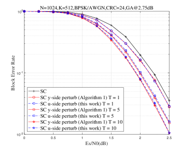
(a) BLER performance comparisons between different perturbation-enhanced SC decoders: $y$-side (Algorithm 1) and $u$-side (Algorithm 2) for a code $(N,K+crc)=(1024,512+24)$ with maximum attempts $T=\{1,5,10\}$ and CRC generator polynomial $g(x)=x^{24}+x^{23}+x^{6}+x^{5}+x+1$.

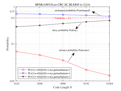
(b) The delay, unchanged, and advance probabilities (2), (3), (4) for code lengths $N=\{1024,2048,4096,8192,16384\}$, code rate $R=\frac{1}{2}$, and design SNRs $\{2.75,2.5,2.25,2,1.85\}$ dB, with a fixed BLER of $10^{-2}$, using $u$-side perturbation-enhanced SC decoding with $T=1$.

Figure 1: Performance analysis of two perturbation-enhanced SC decoders: $y$-side (Algorithm 1) vs $u$-side (Algorithm 2).

All simulations utilize perturbation methods from Algorithm 1 and Algorithm 2 in a BI-AWGN channel with perturbation noise $\sigma_{p}^{2}=10^{-\frac{\text{SNR}-0.1}{10}}-\sigma^{2}$ [13], where SNR is the signal-to-noise ratio, consistently across all code lengths. Decoding is performed until 400 errors are detected for each code length.

In Fig. 1 (a), the red solid line and the blue dashed line represent the performances of the $y$-side (Algorithm 1) and $u$-side (Algorithm 2) perturbation-enhanced SC decoders, respectively. Their nearly identical performance supports further exploration of perturbed decision LLRs in SC decoders.

Fig. 1 (b) shows that as $N$ increases, the delay probability of the $u$-side perturbation-enhanced SC decoder tends to $\frac{1}{2}$, and the advance probability decreases to 0, indicating that perturbation either preserves or improves the SC decoder’s performance with probability $\frac{1}{2}$.

V conclusions

In this paper, we analyze the delay probability of the first error position and show that adding perturbation does not degrade SC decoder’s performance. Our results indicate that the delay probability asymptotically approaches $\frac{1}{2}$, suggesting a potential performance improvement with probability $\frac{1}{2}$. Future research will explore the effects of different perturbation powers on delay probability for a fixed $N$ and develop methods for selecting the optimal perturbation power $\sigma_{p}^{2}$.

References

• [1] E. Arıkan, “Channel Polarization: A Method for Constructing Capacity-Achieving Codes for Symmetric Binary-Input Memoryless Channels,” IEEE Trans. Inf. Theory, vol. 55, no. 7, pp. 3051–3073, Jul. 2009.
• [2] 3GPP TSG RAN WG1, R1-167703, “Channel coding scheme for URLLC, mMTC and control channels,” Intel Corporation, Aug. 2016.
• [3] I. Tal, and A. Vardy, “List Decoding of Polar Codes,” IEEE Trans. Inf. Theory, vol. 61, no. 5, pp. 2213-2226, May 2015.
• [4] A. Balatsoukas-Stimming, M. B. Parizi, and A. Burg, “LLR-based successive cancellation list decoding of polar codes,” IEEE Trans. Signal Process., vol. 63, no. 19, pp. 5165–5179, Oct. 2015.
• [5] K. Niu, and K. Chen, “CRC-Aided Decoding of Polar Codes,” IEEE Commun. Lett., vol. 16, no. 10, pp. 1668-1671, Oct. 2012.
• [6] L. Chandesris, V. Savin, and D. Declercq, “Dynamic-SCFlip decoding of polar codes,” IEEE Trans. Commun., vol. 66, no. 6, pp. 2333–2345, Jun. 2018.
• [7] M. Geiselhart, A. Elkelesh, M. Ebada, S. Cammerer, and S. ten Brink, “On the automorphism group of polar codes,” in Proc. IEEE Int. Symp. Inf. Theory, July. 2021, pp. 1230–1235.
• [8] C. Pillet, V. Bioglio and I. Land, “Polar Codes for Automorphism Ensemble Decoding,” in Proc. IEEE Inf. Theory Workshop (ITW), Oct. 2021, pp. 1-6.
• [9] L. Johannsen, C. Kestel, M. Geiselhart, T. Vogt, S. ten Brink, and N. Wehn, “Successive Cancellation Automorphism List Decoding of Polar Codes,” in 12th Inter. Symp. on Topics in Coding (ISTC), 2023.
• [10] F. Cheng, A. Liu, Y. Zhang, and J. Ren, “Bit-flip algorithm for successive cancellation list decoder of polar codes,” IEEE Access, vol. 7, pp. 58346–58352, 2019.
• [11] K. Ivanov and R. Urbanke, “Polar codes do not have many affine automorphisms,” in Proc. IEEE Int. Symp. Inf. Theory, Jun. 2022, pp. 2374–2378.
• [12] N. K. Gerrar, S. Zhao, and L. Kong, “CRC-aided perturbed decoding of polar codes,” in Proc. Int. Conf. Wireless Commun. Netw. Mobile Comput., 2018, pp. 18-20.
• [13] X. Wang, H. Zhang, J. Wang, J. Ma, and T. Wen, “Perturbation-enhanced SCL decoder for Polar Codes”, in Proc. IEEE Globecom Workshops (GC Wkshps): Channel Coding beyond 5G, Dec. 2023, pp. 1674-1679.
• [14] P. Trifonov, “Efficient design and decoding of polar codes,” IEEE Trans. Commun., vol. 60, no. 11, pp. 3221–3227, Nov. 2012.
• [15] F. W. Olver, D. W. Lozier, R. F. Boisvert, and C. W. Clark, NIST Handbook of Mathematical Functions, New York, NY, USA: Cambridge Univ. Press, 2010.