Exoplanet Ephemerides Change Observations (ExoEcho). I. Transit Timing Analysis of Thirty-Seven Exoplanets using HST/WFC3 Data

Abstract

abstract

The ExoEcho project is designed to study the photodynamics of exoplanets by leveraging high-precision transit timing data from ground- and space-based telescopes. Some exoplanets are experiencing orbital decay, and transit timing variation (TTV) is a useful technique to study their orbital period variations. In this study, we have obtained transit middle-time data from the Hubble Space Telescope (HST) observations for 37 short-period exoplanets, most of which are hot Jupiters. To search for potential long- and short-term orbital period variations within the sample, we conduct TTV model fitting using both linear and quadratic ephemeris models. Our analysis identifies two hot Jupiters experiencing strong periodic decays. Given the old age of the host stars of the hot Jupiter population, our findings call for a scenario where HJs are continuously being destructed and created. Our study demonstrates the importance of incorporating high-precision transit timing data to TTV study in the future.

abstract

The ExoEcho project is designed to study the photodynamics of exoplanets by leveraging high-precision transit timing data from ground- and space-based telescopes. Some exoplanets are experiencing orbital decay, and transit timing variation (TTV) is a useful technique to study their orbital period variations. In this study, we have obtained transit middle-time data from the Hubble Space Telescope (HST) observations for 37 short-period exoplanets, most of which are hot Jupiters. To search for potential long- and short-term orbital period variations within the sample, we conduct TTV model fitting using both linear and quadratic ephemeris models. Our analysis identifies two hot Jupiters experiencing strong periodic decays. Given the old age of the host stars of the hot Jupiter population, our findings call for a scenario where HJs are continuously being destructed and created. Our study demonstrates the importance of incorporating high-precision transit timing data to TTV study in the future.

1 Introduction

A single transiting planet generally orbits its host star on a Keplerian orbit with a constant orbital period. But recently, studying of the transit timing variations (TTV), where transits no longer appear at a fixed interval, have become an important topic in the exoplanet research field. Significant long- and short-term TTV can be induced by additional bodies in the planetary systems, the tidal interaction between the host star and the planets, planetary mass loss, apsidal precession, line-of-sight acceleration, and the Applegate mechanism (Applegate, 1992; Agol et al., 2005; Holman & Murray, 2005; Lai, 2012; Bailey & Goodman, 2019). TTV analysis not only facilitates the detection of additional planetary companions, but also can be used to characterize orbital resonances and provide insights into the internal structure and composition of exoplanets (Agol et al., 2005; Holman & Murray, 2005; Xie, 2013; Nesvorný & Morbidelli, 2008). Thus, it has become an important tool in exoplanetary research field, revealing key properties of planetary systems that might otherwise remain undetected (Jontof-Hutter et al., 2015; Deck & Agol, 2015; Wang et al., 2018, 2021; Ivshina & Winn, 2022; Kokori et al., 2022; Wang et al., 2024). Measuring orbital period variations in exoplanets through the TTV measurements can enhance our understanding of their formation theory, as the current orbital dynamic properties of a system retains information about its past evolution history. Patra et al. (2020) have searched evidence for tidal orbital decay using transit-timing data of twelve hot Jupiters. Yee et al. (2020) found secular decay in the orbital period of WASP-12 b using TTV measurements, which they attribute to the tidal interaction between the planet and its hot star (see also Turner et al., 2021; Wang et al., 2024). By analyzing 28 yrs of TTV observation, Maciejewski et al. (2020) have put a constraint on the tidal quality factor of the host star of WASP-18 b. Davoudi et al. (2021) gave a lower limit on the tidal quality factor of WASP-43 by measuring the mid-transit times of WASP-43 b. TTV studies also have significant implications for planning future follow-up transit observations, where an accurate transit window prediction is needed Kokori et al. (2022). For example, Barker (2020) have provided predictions for shifts in transit times due to tidally driven orbital decay of exoplanets. Most of the past exoplanet TTV studies have utilized data from various sources, including space-based telescopes and ground-based observatories (Mazeh et al., 2013; Holczer et al., 2016; Hadden & Lithwick, 2017; Sun et al., 2017; Kane et al., 2019; Ivshina & Winn, 2022; A-thano et al., 2023; Wang et al., 2021, 2024). Despite significant advancements in the TTV research field, many of these studies are limited by their reliance on archival data from diverse observational projects, a substantial portion of which is ground-based and thus susceptible to many unknown systematics (Mallonn et al., 2019; Ivshina & Winn, 2022; Alvarado et al., 2024; Wang et al., 2024). In this paper, we propose the incorporation of data from the Hubble Space Telescope (HST) into the study of TTVs of exoplanets, as part of our ExoEcho project. The ExoEcho (Exoplanet Ephemerides CHange Observation) project is designed to study the photodynamics of exoplanets by leveraging high-precision transit timing data from ground- and space-based telescopes. In our previous two papers (Wang et al., 2024; Zhang et al., 2024), we have studied the TTV behaviors of hot Jupiters mostly using the TESS (Ricker, 2015) mission data. By integrating the high precision and reliable HST timing data into the TTV modeling, we expect to put more precise constraints on the TTV properties of exoplanets and identify new candidates exhibiting signs of long- and short-term orbital period variations. The paper is organized as follows: In Section 2, we introduce the transit timing data used in this study. Section 3 presents our analysis methods, including the algorithms and models applied to extract and interpret the TTV signals. In Section 4, we present the TTV results for all thirty-seven exoplanet systems in our sample. A detailed discussion of our findings and their implications for planetary system formation and evolution is presented in Section 5. Finally, we conclude this study with a summary in Section 6.

2 Sample Selection and Data Analysis

2.1 Sample Selection

Here we select short orbital period transiting exoplanets from Wang et al. (2024), which have early transiting data and observed by the HST and the TESS, providing an important longer-time baseline for analyzing long-term orbital period variations. In the end, our sample consists of 37 exoplanets, ranging from warm Neptunes to hot Jupiters. We summarize the stellar and planetary parameters for these systems in Table 1. All the selected exoplanets have an orbital period $\lesssim 10$ days.

Table 1: Stellar and Planetary Parameters of Selected Exoplanet Systems

Planet	[Fe/H]⋆	$T_{\star}$	log ($g_{\star}$)	$M_{p}$	$R_{p}/R_{\star}$	$P$	$i$	$a/R_{\star}$	$e$	$\omega$	Ref.
		(K)	(cgs)	($M_{\mathrm{\rm Jup}}$)		(days)	(deg)			(deg)
HAT-P-2 b	0.12	6290	4.2	9.04	0.07227	5.63346785	86.72	8.99	0.5171	185.22	1; 2; 3; 4; 5; 6; 7
HAT-P-3 b	0.27	5185	4.56	0.596	0.1063	2.89973815	87.1	10.4	…	…	8; 3; 9; 6; 10; 14
HAT-P-11 b	0.31	4780	4.6	0.081	0.0576	4.88780201	88.5	15.58	0.2	355.2	11; 5; 12
HAT-P-12 b	-0.29	4650	4.61	0.211	0.1406	3.21305762	89	11.77	…	…	13; 5; 6; 10; 14
HAT-P-17 b	0	5246	4.52	0.534	0.1238	10.33853522	89.2	22.6	0.342	201	15; 5; 6
HAT-P-18 b	0.1	4803	4.57	0.197	0.1356	5.50802941	88.53	16.39	…	…	16; 17; 5; 6; 18
HAT-P-24 b	-0.16	6373	4.27	0.685	0.097	3.35524439	88.6	7.6	0.067	197	19; 5; 6
HAT-P-26 b	-0.04	5079	4.56	0.059	0.0737	4.2345002	88.6	13.1	0.12	54	20; 5
HAT-P-32 b	-0.04	6207	4.329	0.68	0.1489	2.150008197	89	5.34	0.16	50	21; 22; 5; 6
HAT-P-38 b	0.06	5330	4.46	0.267	0.0918	4.64032787	88.3	12.2	0.07	240	23; 6
HAT-P-41 b	0.21	6390	4.14	0.812	0.1028	2.69404968	87.7	5.44	…	…	24; 6
HD 97658 b	-0.23	5170	4.63	0.02375	0.0311	9.4893037	89.8	26.2	…	…	25; 26; 27; 28; 29
KELT-7 b	0.14	6789	4.15	1.28	0.091	2.7347656	83.8	5.53	…	…	30
KELT-11 b	0.18	5370	3.73	0.195	0.051	4.7362006	85.3	4.98	0.0007	359	31; 32
TrES-4 b	0.14	6200	4.06	0.84	0.1045	3.55392889	83.1	6.14	…	…	33; 5; 6; 34
WASP-4 b	0	5500	4.3	1.186	0.152	1.338231388	89.1	5.451	…	…	35; 36; 5; 6; 37;
WASP-6 b	…	5450	4.5	0.503	0.1446	3.36100215	88.5	10.9	0.054	1.7	38; 6
WASP-12 b	0.3	6300	4.18	1.47	0.1178	1.091419179	83.4	3.04	…	…	39; 40; 5; 6
WASP-17 b	-0.25	6550	4.24	0.486	0.1235	3.73548545	87.1	7.03	…	…	41; 42; 43; 5; 6; 37
WASP-18 b	0	6400	4.4	10.3	0.09716	0.941452417	84.9	3.562	0.0091	269	44; 45; 5; 6; 37
WASP-19 b	0.2	5500	4.5	1.069	0.1409	0.788839092	78.8	3.46	0.002	259	46; 47; 5; 6; 48
WASP-29 b	0.11	4800	4.54	0.244	0.0982	3.92271183	89.2	12.36	…	…	49; 50; 6;
WASP-39 b	-0.12	5400	4.498	0.283	0.1457	4.05528043	87.75	11.37	…	…	51; 52; 6; 10
WASP-43 b	-0.05	4400	4.64	1.78	0.1594	0.813474056	82.11	4.867	…	…	53; 54; 6; 55;
WASP-62 b	0.04	6280	4.32	0.57	0.1109	4.41193868	88.3	9.52	…	…	56; 6; 57
WASP-63 b	0.08	5570	4.01	0.38	0.078	4.37808205	87.8	6.49	…	…	56; 6
WASP-69 b	0.14	4715	4.54	0.26	0.1336	3.86813888	86.71	11.953	…	…	58; 6; 59
WASP-76 b	0.23	6250	4.13	0.92	0.109	1.80988043	88	4.07	…	…	60; 61
WASP-79 b	0.03	6600	4.06	0.9	0.113	3.66239163	85.4	7.02	…	…	62; 6; 57
WASP-80 b	-0.14	4145	4.69	0.538	0.1714	3.06785251	89.02	12.63	0.002	94	63; 64; 6
WASP-96 b	0.14	5540	4.42	0.48	0.1175	3.42525674	85.6	9.255	…	…	65; 6
WASP-98 b	-0.6	5525	4.58	0.922	0.1582	2.96264191	86.38	10.92	…	…	65; 66; 6
WASP-101 b	0.2	6400	4.34	0.5	0.1122	3.585707	85	8.445	…	…	65; 6
WASP-117 b	-0.11	6038	4.28	0.2755	0.09	10.0205933	89.1	17.4	0.302	242	67; 6
WASP-121 b	0.13	6459	4.24	1.183	0.1245	1.274924762	87.6	3.754	…	…	68; 69
WASP-127 b	-0.18	5620	4.18	0.18	0.1004	4.17806513	88.2	7.95	…	…	70; 71
WASP-178 b	0.21	9350	4.35	1.66	0.1115	3.3448285	85.7	7.17	…	…	72; 73

2.2 Hubble Data

For the 37 exoplanets in our sample, we download their HST/WFC3 slitless spectroscopy transit observation data (STScI, 2016) with the IR G102 or G141 grism from the NASA Mikulski Archive for Space Telescopes archive. All observations are executed in the spatial scanning mode, which can maximize the signal-to-noise ratio and avoid saturation for these bright targets. A complete list containing the observation proposal information, the number of transits covered, and the HST orbits spent for the observation are shown in Table 2. Most of our targets have one to five transits covered by the HST observations.

Table 2: HST Observations Analyzed

				HST
			Transits	Orbits
Planet	Proposal ID	Proposal PI	Covered	Used
HAT-P-2 b	16194	Jean-Michel Desert	1	5
HAT-P-3 b	14260	Drake Deming	2	8
HAT-P-11 b	12449	Drake Deming	1	3
HAT-P-11 b	14793	Jacob Bean	5	15
HAT-P-12 b	14260	Drake Deming	2	8
HAT-P-17 b	12956	Catherine Huitson	1	4
HAT-P-18 b	14099	Thomas Evans-Soma	1	3
HAT-P-18 b	14260	Drake Deming	2	8
HAT-P-24 b	16736	David Sing	1	4
HAT-P-24 b	16587	Frederick Dauphin	…	…
HAT-P-26 b	14110	David Sing	1	4
HAT-P-26 b	14260	Drake Deming	2	8
HAT-P-32 b	14260	Drake Deming	1	4
HAT-P-38 b	14260	Drake Deming	2	8
HAT-P-41 b	14767	David Sing	1	4
HD 97658 b	13501	Heather Knutson	1	4
HD 97658 b	13665	Bjorn Benneke	2	8
KELT-7 b	14767	David Sing	1	4
KELT-11 b	15926	Knicole Colon	1	8
KELT-11 b	15255	Knicole Colon	1	7
TrES-4 b	12181	Drake Deming	1	4
WASP-4 b	12181	Drake Deming	1	4
WASP-6 b	14767	David Sing	1	4
WASP-12 b	13467	Jacob Bean	4	16
WASP-12 b	12330	Mark Swain	1	4
WASP-12 b	16236	Taylor Bell	1	4
WASP-17 b	14918	Hannah Wakeford	3	12
WASP-17 b	12181	Drake Deming	1	4
WASP-18 b	12181	Drake Deming	1	4
WASP-19 b	12181	Drake Deming	1	4
WASP-29 b	14260	Drake Deming	1	4
WASP-39 b	14260	Drake Deming	1	4
WASP-43 b	13467	Jacob Bean	4	16
WASP-62 b	14767	David Sing	1	4
WASP-63 b	14642	Kevin Stevenson	1	7
WASP-69 b	14260	Drake Deming	1	3
WASP-76 b	14767	David Sing	1	4
WASP-79 b	14767	David Sing	1	4
WASP-80 b	14260	Drake Deming	1	3
WASP-96 b	15469	Nikolay Nikolov	1	4
WASP-98 b	16736	David Sing	1	3
WASP-101 b	14767	David Sing	1	4
WASP-117 b	15301	Ludmila Carone	1	10
WASP-121 b	15134	Thomas Evans-Soma	1	4
WASP-121 b	14468	Thomas Evans-Soma	1	4
WASP-127 b	14619	Jessica Spake	1	4
WASP-178 b	16450	Joshua Lothringer	2	8

Note. — The HAT-P-24’s proposal 16587 provides the flt.fits file for proposal 16736.

The data reduction for transit observation from HST/WFC3 is the same as in our previous studies (Zhou et al., 2022, 2023). We start our data reduction from the raw HST/WFC3 spatially scanned spectroscopic images using Iraclis (Tsiaras et al., 2016a, b, 2018). The basic calibration includes the following steps: zero-read subtraction, reference pixels correction, non-linearity correction, dark current subtraction, gain conversation, sky background subtraction, calibration, flat-field correction, and bad pixels/cosmic rays correction. Following the basic calibration, 1D spectra are extracted using the standard optimal extraction technique (Horne, 1986; Piskunov & Valenti, 2002; Zechmeister et al., 2014; Ma & Ge, 2019; Cornachione et al., 2019). An example of the extraction region and the corresponding extracted 1D spectrum are presented in Figures 1 and  2. We sum the G141 spectrum from 1.1 to 1.7 $\mu$m or the G102 spectrum from 0.8 to 1.15 $\mu$m to obtain raw white light curves of transiting exoplanets from each exposure, as shown in the top panel of Figure 3. Outliers are then removed from the final raw white light curves.

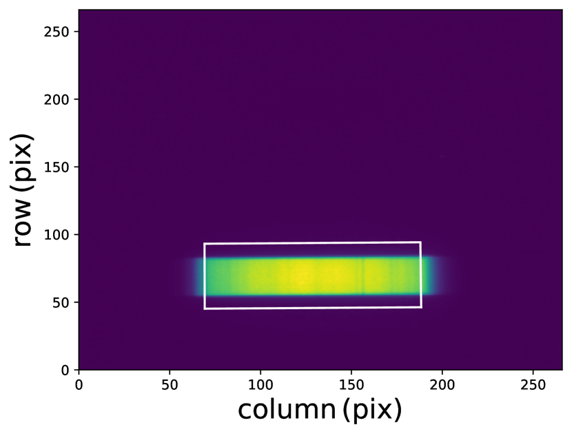
Figure 1: The detector image of a forward scan

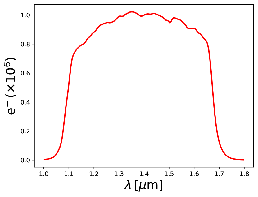
Figure 2: Extracted 1D spectrum using Iraclis

We obtain the middle transit time parameter $T_{\rm mid}$ for each transit observation by fitting all the raw white light curves with the transit model from Mandel & Agol (2002). During the fitting process, we fix the stellar, planetary, and orbital parameters to values from literature (see Table 1) and allow only $T_{0}$ and $R_{p}/R_{\star}$ to vary as free parameters. We model the stellar limb-darkening effect using the nonlinear formula proposed by Claret (2000). The limb-darkening coefficients are derived from specific intensity profiles evaluated at 100 angles, calculated directly from the ATLAS model (Howarth, 2011), as all our target stars have effective temperatures above 4,000 K (see Table 1). To correct for time-dependent systematics in the HST/WFC3 observations (Kreidberg et al., 2015; Wakeford et al., 2016; Evans et al., 2016; Line et al., 2016; Wakeford et al., 2017a; Tsiaras et al., 2018), we fit the transit model together with a normalization factor $n_{w}$ and an instrumental systematics function $R(t)$, following the studies of Kreidberg et al. (2014) and Tsiaras et al. (2016a, 2018). To double check the fitting result of the Iraclis package, we also fit the raw white light curves using the PyTransit (Parviainen, 2015) and batman (Kreidberg, 2015) packages. We adopt the fitting result from the PyTransit fitting when we deem it feasible. In the end, we obtain a total of 64 mid-transit times for the 37 planetary systems in our sample, which are summarized in Table 3.

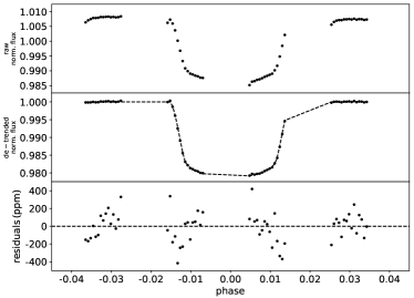
Figure 3: Top: the normalized raw white light curve of HAT-P-12 from the 2015 observation from HST/WFC3 (PI: Drake Deming, Proposal ID: 14260). Middle: the same raw white light curve divided by the best-fit model of the instrument systematics. Bottom: residuals from the best-fit transit model light curve.

Table 3: Middle transit times extracted by fitting the raw white light curves from the HST/WFC3 observation.

Planet	Proposal ID	$T_{\rm mid}(\mathrm{BJD_{TDB}})$	Uncertainty (days)	Tools
HAT-P-2 b	16194	2459204.10902	0.0002345	I

Note. — Table 3 is fully published in a machine-readable format, with a sample provided here for reference.

3 Modeling of the Transit Times Data

In this section, we utilize the middle transit times extracted from the HST/WFC3 data in this study, along with archival transit times from the database of Wang et al. (2024) and Ivshina & Winn (2022), to study the transit timing variations (TTVs) of the planets in our sample. For TESS observation, we adopt only results from the study of Wang et al. (2024).

3.1 Transit-timing Models

TTV studies utilize two popular models: the constant period model and the constant period derivative model (eg: Maciejewski et al., 2016b; Patra et al., 2017; Wang et al., 2024). We use the MCMC method to fit these models to the data of the transit middle times. The first model assumes a linear ephemeris with a constant orbital period $P$:

$$T_{n}=T_{0}+nP$$ (1)

where n is the transit number counting from the zero reference middle transit time $T_{0}$, and $T_{n}$ is time of the n-th transit. The second model assumes a quadratic ephemeris that the period changes at a constant rate:

$$T_{n} = T_{n-1}+P_{n-1},$$ (2)

$$P_{n} = P_{n-1}+\frac{P_{n-1}+P_{n}}{2}\dot{P},$$ (3)

where the period change rate, denoted by $\dot{P}$, is defined as $\frac{dP}{dt}=\frac{1}{P}\frac{dP}{dn}$. This recursive formula utilizes past values to compute subsequent values in a sequence. The three parameters used in the second model are the zero reference transit time $T_{0}$ corresponding to the zero epoch, the orbital period $P_{0}$ at $T_{0}$, and the constant period change rate $\dot{P}$.

3.2 Transit Timing Data Analysis

We use the transit timing data analysis tool PdotQuest (Wang et al., 2024) to fit the transit middle time for both models. In our MCMC analysis (Goodman & Weare, 2010; Foreman-Mackey et al., 2013), we utilize 100 walkers to explore the parameter space, with each walker completing 500 steps. To ensure convergence, we discarded the first 100 steps of each walker as burn-in. For all the fitting parameters, we use uniform priors. To identify and exclude outliers, we apply an iterative fitting method known as ‘n-$\sigma$ rejection’. This method involves calculating the standard deviation of the fitting residuals and removing any data points with residual values exceeding the n-sigma threshold from the residual mean. Specifically, we explore the fitting results from within the 5-$\sigma$ and 3-$\sigma$ ranges. The Bayesian Information Criterion (BIC) is a statistical tool for model selection among a finite set of competing models (Schwarz, 1978). In this study, we employ BIC to compare fitting results from both of the linear and quadratic models, while accounting for model complexity. BIC is calculated as $BIC=\chi^{2}+klogn$, where k is the number of parameters, and n is the number of observation data points. Lower BIC values suggest better-fitting models and $\Delta BIC>10$ indicates strong evidence of the model with the lower BIC (Kass & Raftery, 1995). We identify long-term period changes in the samples using two criteria: (a) the period derivative $\dot{P}$ must be at least 3-$\sigma$ away from zero, indicating a significant deviation from a constant period, and (b) the difference in Bayesian Information Criterion ($\Delta BIC=BIC_{linear}-BIC_{quadratic}$) must exceed 10, suggesting strong evidence in favor of the model with the lower BIC. In the study of Ivshina & Winn (2022) and Wang et al. (2024), they have also mentioned one single data point with unrealistically small error bar will produce false positives when looking for orbital period decay using TTV method. To validate our fitting results, we use the leave-one-out cross-validation (LOOCV) test following Wang et al. (2024). This test iteratively removes a data point and re-fits the remaining data to assess the impact of one data point on the model fitting.For some data points identified by the LOOCV test that can significantly affect the fitting results, we also explore different TTV fitting solutions by not simply removing the data point but modifying its error bar in the following way. If the error bar of one data point identified by LOOCV is less than 0.0003 days, we will enlarge it to 0.0003 days or three times its original value, whichever is smaller, and re-do the fitting. By conducting this additional test, we can have more robust quadratic model fitting results, which are less impacted by transit time data having unreliably small error bars. Out of the 37 planets in our sample, three have undergone the additional testing procedure.

4 Results

In this section, we present the model fitting and testing results for all the planets in our sample. After examining the result of each target, we divide the whole sample into four different categories: 6 systems showing signs of long-term period variation, 4 systems showing signs of short-term period variation, 8 systems as ‘interesting’, and 19 systems showing no signs of period variation. The final ephemerides derived in this work are made available online. We will discuss individual systems from the first three categories next. All fitting results for the remaining 19 systems belonging to the fourth category are shown in Figure A1 in the Appendix.

4.1 Long-term period changes

We initially have 6 systems that show strong evidence of possible long-term period variation. However, only 2 of them have passed the LOOCV test. All their fitting and LOOCV test results are shown in Figure 4.

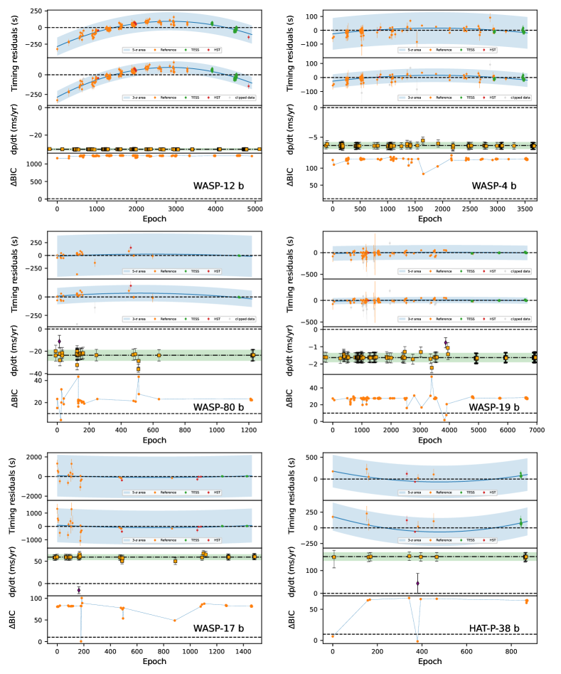
Figure 4: Time residuals from TTV fitting, LOOCV analysis, and corresponding $\Delta BIC$ of exoplanets studied in Section 4.1. For each exoplanet: Top panel: time residual results using 5-$\sigma$ rejection scheme. The second panel: time residual results using 3-$\sigma$ rejection scheme. The blue curves and shaded areas indicate the best-fit quadratic model. Orange points are based on previous literature data. Green points are based on TESS data. Red points are based on HST data from this work. Gray points are clipped data. The third panel shows the period change rate $dp/dt$ from fitting a quadratic model after removing each transit timing data point. Orange squares indicate $dp/dt$ values 3-$\sigma$ away from zero, while purple diamonds represent values within 3-$\sigma$. The dash-dotted line marks the original $dp/dt$ fit, with the green shaded area showing the 1$\sigma$ confidence region. The bottom panel displays the corresponding $\Delta BIC$.

• WASP-12 b is an ultra hot Jupiter with mass of $1.5~M_{\rm Jup}$ and orbital period of 1.1 day around a later-F star (Hebb et al., 2009; Collins et al., 2017). Previous TTV studies have indicated a decreasing trend in its orbital period (Maciejewski et al., 2016b; Patra et al., 2017). Yee et al. (2020) presented new transit and occultation observations that provide more decisive evidence for the orbital decay of WASP-12 b. Turner et al. (2021) analyzed data from TESS to verify that WASP-12b’s orbit is indeed changing with an updated decay rate of $32.53\pm 1.62$ ms/yr. Bai et al. (2022) also found a significant change in the planetary orbit using telescopes of Yunnan Observatories. Ivshina & Winn (2022) reported $\dot{P}=-30.27\pm 1.11$ ms/yr and Wang et al. (2024) found $\dot{P}=-30.19\pm 0.92$ ms/yr. In this study, by incorporating HST data, we obtain $\dot{P}=-30.31\pm 0.85$ ms/yr and $\Delta BIC=1241$, further confirming its orbital decay nature. We estimate its $Q^{\prime}_{*}>1.7\times 10^{5}$ using Equation (1) of Patra et al. (2020).

• WASP-4 b is a $1.2~M_{\rm Jup}$ hot Jupiter with a 1.3 day orbital period around a G7V star (Wilson et al., 2008). Bouma et al. (2019) identified an orbital period decay rate of about 10 ms/yr in WASP-4 b, using data from TESS and ground-based transit observations. Based on new radial-velocity (RV) measurements and speckle imaging observation, Yee et al. (2020) inferred that the decrease is most likely caused by the line-of-sight acceleration of the system. Turner et al. (2022) examined TESS, RV, and archival transit data, revealing no Earthward acceleration in the full RV dataset. They suggested a possible additional planet in the system, but its presence could not explain the observed period decay. Instead, they suggested there exists either an orbit decay with $\dot{P}=-7.33\pm 0.71$ ms/yr or apsidal precession in the system. Harre & Smith (2023) analyzed TESS and archival data of WASP-4 b but found no conclusive cause for its apparent transit timing variations. Using TESS data, Ivshina & Winn (2022) obtained $\dot{P}=-5.81\pm 1.58$ ms/yr and Wang et al. (2024) obtained $\dot{P}=-6.43\pm 0.55$ ms/yr for WASP-4 b. Here in this study, by adding HST data to the fitting, we find $\dot{P}=-6.46\pm 0.58$ ms/yr and $\Delta BIC=127$, which confirms the orbital decay. We estimate its $Q^{\prime}_{*}>5.7\times 10^{4}$ using Equation (1) of Patra et al. (2020).

• WASP-80 b is a planet with a mass of $0.54~M_{\rm Jup}$ and an orbital period of 3.1 day around a cool dwarf star (Triaud et al., 2013, 2015). Our analysis shows a decay in the orbital period at a rate of $-23.58\pm 4.95$ ms/yr, and $\Delta BIC=19$. LOOCV test results indicate that one key data point significantly affects the TTV fitting result. We then refit the model after inflating the error bar of this data point to 3 times its original value, which gave a $\dot{P}$ result of $-10.80\pm 5.65$ ms/yr, more consistent with a constant period model.

• WASP-19 b is a $1.1~M_{\rm Jup}$ planet with a 0.79 day orbital period orbiting a G8-type star (Hebb et al., 2010; Wong et al., 2016). Patra et al. (2020) found strong evidence of orbital decay, but disputed later by studies like Petrucci et al. (2020) and Wang et al. (2024). The overall data fitting initially shows a slight period decrease trend, with a rate of $-1.64\pm 0.28$ ms/yr and $\Delta BIC=33$. After re-fitting data with the error bars enlarged, the trend disappears ($\dot{P}=-0.26\pm 0.30$ ms/yr). Thus, we need to continue monitoring this target in the future.

• WASP-17 b is an ultra-low-density planet with a mass of $0.49~M_{\rm Jup}$ and a radius of $2.0~R_{\rm Jup}$, which orbits an F6-type star with sub-solar metallicity. It has an orbital period of 3.7 days (Anderson et al., 2010, 2011). The period initially appears to be increasing with a best-fit rate of $59.01\pm 6.56$ ms/yr and $\Delta BIC=82$. We then perform the LOOCV test, which identifies a key data point that strongly affects the fitting result. When re-fit the data with this key data point’s error bar enlarged by a factor of three, we find no strong evidence supporting this long-term orbital period variation, with $\dot{P}=19.63\pm 7.17$ ms/yr.

• HAT-P-38 b is a planet with a mass of 0.27 $M_{\rm Jup}$ and an orbital period of 4.6 day around a late G star (Sato et al., 2012). It belongs to a rapidly increasing population of transiting Saturn-like planets, and transmission spectra observation has revealed a relatively clear atmosphere with a clear detection of water (Bruno et al., 2018). We find that the orbital period is increasing at a rate of $161.10\pm 18.79$ ms/yr, with a $\Delta BIC$ of 66. However, the LOOCV test shows one of our two HST data points strongly affects the fitting result. When re-fitting after rejecting this HST data point, we find a result consistent with a constant period model, with $\dot{P}=42.63\pm 45.93$. Thus, Further observations are needed to verify this trend.

4.2 Short-term TTV

Although some systems do not exhibit trends in long-term orbital period variations, they may show potential short-term transit timing variations (TTVs). In this section, we present four such systems. All their fitting results are shown in Figure 5. These systems are worth further study to identify the exact reasons behind these variations.

• HAT-P-2 b (also called HD 147506 b) is a hot Jupiter wit mass of $9.04~M_{\rm Jup}$, eccentricity of 0.52, and orbital period of 5.6 day, which orbits around a bright F8 star (Bakos et al., 2007). The study of Jacobs et al. (2024) reveals the rapid heating and cooling of this highly eccentric hot Jupiter, which they attribute to the possible star-planet interaction. de Beurs et al. (2023) have studied its orbital period evolution using simulation and suggested further monitoring it with precise RVs and transit and eclipse timings. Our fitting results suggest the potential presence of short-term TTVs with an amplitude as large as 100 s, which may be related to the system’s strange large eccentricity.

• HAT-P-11 b is a $0.081~M_{\rm Jup}$ planet with an orbital period of 4.9 day, orbiting a bright and metal rich K4-type dwarf star (Bakos et al., 2010). Yee et al. (2018) discovered a second planet HAT-P-11 c in this system. With this additional companion, the eccentricity and stellar obliquity of HAT-P-11 b could be explained under the assumption that HAT-P-11 c was also misaligned. Lu et al. (2024) proposed a two-step dynamical process that can reproduce all observed properties of this system. Our TTV fitting results show that short-term strong variations exist in this system, which awaits future confirmation.

• HAT-P-18 b is a $0.20~M_{\rm Jup}$ planet with an orbital period of 5.5 day, orbiting a K2 dwarf star (Hartman et al., 2011a). Our fitting results indicate that neither the long-term constant-period model nor the quadratic model provides a satisfactory fit, suggesting the possible presence of short-term TTVs with an amplitude as large as 100 s in this system.

• WASP-178 b is a bloated planet with a mass of $1.7~M_{\rm Jup}$, radius of $1.81~R_{\rm Jup}$, and orbital period of 3.3 day, which orbits around an A1V-type star with an effective temperature of $9350$ K (Hellier et al., 2019). Our fitting results indicate that neither the long-term constant-period model nor the quadratic model provides a satisfactory fit, suggesting the possible presence of short-term TTVs with an amplitude as large as 250 s in this system.

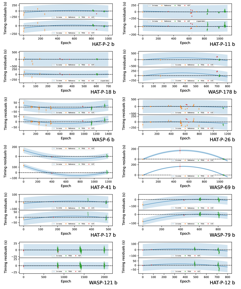
Figure 5: Time residuals of exoplanets in Section 4.2 and Section 4.3

4.3 Special Interest

In this section, we present 8 systems that are classified as ‘interesting’ by us, including planets showing possible weak period variation, and targets showing significantly different results between this study and the literature. All their fitting results are shown in Figure 5. All of these targets warrant further observations.

• WASP-6 b is an inflated sub-Jupiter mass planet, with with a mass of $0.50~M_{\rm Jup}$ and radius of $1.2~R_{\rm Jup}$, indicating that it has a puffed-up, extended atmosphere. It orbits around a mildly metal-poor solar-type star with a 3.4 day orbital period (Gillon et al., 2009a). The orbital period was found to be increasing by Wang et al. (2024), and adding new HST data further constrains the rate of orbital period change. Our analysis yields a rate of $16.21\pm 4.77$ ms/yr and $\Delta BIC=9$, which is close to the value obtained by Wang et al. (2024) ($\dot{P}=20.66\pm 5.19$ ms/yr). The LOOCV test indicates that the first data point has greatly affected the fitting result. We then refit the model after inflating the error bar of this data point to 3 times its original value, which shows a $\dot{P}$ value of $11.99\pm 5.27$ ms/yr, consistent with a constant period model.

• HAT-P-26 b is a low-density planet with a mass of $0.059~M_{\rm Jup}$ and an orbital period of 4.2 day around a K1-type dwarf star (Hartman et al., 2011b). Its mass, comparable to Neptune and Uranus, coupled with a radius approximately 65% larger than those of Neptune and Uranus, sets HAT-P-26b apart from other transiting Super-Neptunes (Hartman et al., 2011b). HAT-P-26b exhibits a well-constrained heavy element abundance, which is lower than that observed in Uranus and Neptune (Wakeford et al., 2017b; MacDonald & Madhusudhan, 2019). A-thano et al. (2023) suggested the $1.98\pm 0.05$ minute amplitude signal in the TTV analysis could be due to a $0.02~M_{\rm Jup}$ planet in a 1:2 resonance orbit. When we use our processed HST data along with literature data, fitting shows a constant period ($\dot{P}=-20.60\pm 11.72$ ms/yr). However, if we fit the data with previous HST data, we observe a significant increasing trend in the period ($\dot{P}=119.64\pm 9.12$ ms/yr).

• HAT-P-41 b is a $0.80~M_{\rm Jup}$ planet with an orbital period of 2.7 day, orbiting a moderately bright (V=12.4) F star (Hartman et al., 2012). We initially identify an increasing trend in its orbital period using archival data and our TESS and HST data, with $\dot{P}=86.32\pm 27.08$ ms/yr and $\Delta BIC=8$. We later find the only one archival data used in the fitting from Wakeford et al. (2020) is actually a combined epoch data from many observations of Spitzer and HST spanning 10 years. We then go ahead to use individual timing data from literature instead of this one combined data (Hartman et al., 2012; Wakeford et al., 2020), and re-fit the TTV model. The increasing trend disappears at this time, with $\dot{P}$ as $-7.68\pm 13.07$ ms/yr.

• WASP-69 b is a bloated Saturn-mass planet with a mass of $0.26~M_{\rm Jup}$, a radius of $1.1~R_{\rm Jup}$, and an orbital period of 3.9 day around an active, mid-K-type dwarf star (Anderson et al., 2014). Recently, through X-ray and extreme ultraviolet (XUV) bands research, Levine et al. (2024) discovered that WASP-69 b may experience atmospheric dissipation. In our study, the decreasing period trend only meets a 2 sigma criterion with $\dot{P}=-117.92\pm 41.77$ ms/yr and does not satisfy the $\Delta BIC$ criterion, suggesting a weak trend awaiting further confirmation.

• HAT-P-17 b is a hot Jupiter with a mass of $0.53~M_{\rm Jup}$ and an orbital period of 10 day around an early K-type dwarf star (Howard et al., 2012). It is situated in a multi-planet system. The inner planet has an eccentric, short-period orbit, while the outer planet, HAT-P-17 c, is a cold Jupiter with a nearly circular orbit and a period of 4.4 years (Howard et al., 2012). While our analysis indicates a potential decreasing trend with $\dot{P}=-29.43\pm 15.72$ ms/yr, the limited data available prevents the results from meeting the statistical ’strong’ criteria.

• WASP-79 b is a highly-bloated planet with a mass of $0.9~M_{\rm Jup}$ and orbital period of 3.7 day around an F-type star (Smalley et al., 2012). Our analysis initially shows a decay in the orbital period at a rate of $-78.80\pm 26.22$ ms/yr, and $\Delta BIC=-1$. We then re-fit the model after removing the first data point and adding data from Brown et al. (2017). This yields a $\dot{P}$ value of $-47.81\pm 19.76$ ms/yr, which is consistent with a constant period model.

• WASP-121 b is a planet with a mass of $1.2~M_{\rm Jup}$ and an orbital period of a 1.3 day around an active F-type star (Delrez et al., 2016). The fitting results show the orbital period is increasing. The fits using both the 3-sigma and 5-sigma rejection schemes do not meet the $\Delta BIC<10$ criterion, but the fitting using a 7-sigma rejection scheme yields a result that meets the $\Delta BIC>10$ criteria. However, if using only data from HST and TESS which we deemed trustworthy, we found a $\dot{P}$ of $0.02\pm 2.01$ ms/yr, showing no evidence of significant period variation. This result also demonstrates the superiority of two HST data points compared to the tens of data points from ground-based telescopes.

• HAT-P-12 b is a low density planet with a mass of $0.21~M_{\rm Jup}$ and orbital period of 3.2 day around a K4-type dwarf star (Hartman et al., 2009). The fitting with all available timing data indicates it has a constant orbital period. However, when fitting only the HST and TESS data, we find the orbital period is decreasing with $\dot{P}=-40.22\pm 17.92$ ms/yr. This new fitting does not yet satisfy the 3-$\sigma$ and $\Delta BIC>10$ criterion. Future high-precision transit timing data are needed to confirm this decreasing trend.

5 Discussion

5.1 Inspiral Timescale of HJs

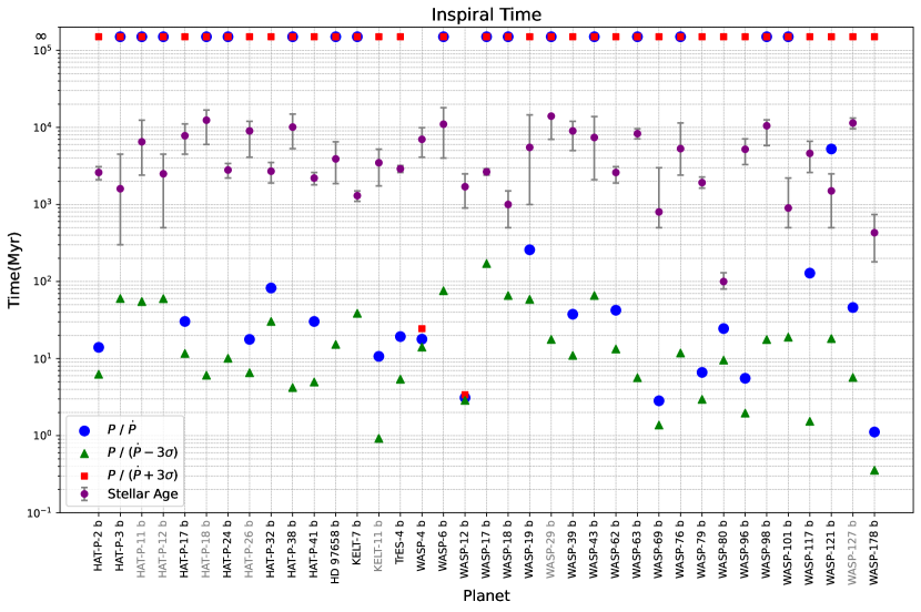
Figure 6: Inspiral Timescale for exoplanets in our sample. Grey: exoplanets with mass $M\lesssim 0.25M_{J}$; Black: HJ ($0.25M_{J}<M\lesssim 13.6M_{J}$). The stellar ages are taken from: Pál et al. (2010); Chan et al. (2011); Bakos et al. (2010); Hartman et al. (2009); Howard et al. (2012); Hartman et al. (2011a); Kipping et al. (2010); Hartman et al. (2011b, c); Sato et al. (2012); Hartman et al. (2012); Ellis et al. (2021); Bieryla et al. (2015); Ghezzi et al. (2018); Bonomo et al. (2017); Petrucci et al. (2013); Gillon et al. (2009a); Anderson et al. (2011); Hellier et al. (2009); Hebb et al. (2010); Hellier et al. (2010); Faedi et al. (2011); Scandariato et al. (2022); Hellier et al. (2012); Anderson et al. (2014); West et al. (2016); Smalley et al. (2012); Triaud et al. (2013); McGruder et al. (2023); Hellier et al. (2014); Delrez et al. (2016); Lam et al. (2017); Rodríguez Martínez et al. (2020).

The formation and evolution of HJs remain a hot topic in the exoplanet research field (Dawson & Johnson, 2018; Zink & Howard, 2023; Wu et al., 2023; Fang et al., 2023). Here, we can contribute to this topic by putting constraints on the in-spiral time scale of the HJs. Assuming the rate of orbital period decay remains constant, the inspiral timescale (or known as orbital decay timescale) is usually defined as:

$$T_{\rm inspiral}=\frac{P}{\dot{P}},$$ (4)

which represents how long it would take for a hot Jupiter to be engulfed by its host star. In Figure 6, we present the distribution of $T_{\rm inspiral}$, along with its 3-$\sigma$ upper and lower limits calculated using a 3-$\sigma$ error in $\dot{P}$. The distribution indicates that most host stars are older than 0.5 Gyr, while some HJs exhibit relatively short inspiral timescales. This finding suggests that certain HJs may undergo the engulfment process within the next several Myr. To date, nearly 400 hot Jupiters (HJs) have been discovered. Our inspiral timescale analysis further implies that, if the current rate of period change remains constant, approximately $0.5\%$ ($\sim 2/400$) of these HJs will be lost within the next $10^{7}$ years. With a linear extrapolation, this trend would predict the disappearance of all HJs within the next $2\times 10^{9}$ years. Consequently, this analysis suggests that the majority of HJs may be expected to be lost over a timescale comparable to the typical ages of their host stars, which are on the order of several Gyr. Given the older ages of HJ host stars, some mechanisms for continuous HJ formation on the timescale up to several Gyr is needed so as to sustain the observed HJ population. This supports the need for a ‘late-arrived’ hot Jupiter population, as proposed by Hamer & Schlaufman (2022), Chen et al. (2023), and Chen et al. (2024, submitted). One possible channel for HJ replenishment is the dynamical high-eccentricity migration (Rasio & Ford, 1996; Chatterjee et al., 2008; Naoz et al., 2012; Petrovich, 2015), a scenario supported by recent observations (Zink & Howard, 2023). However, observations of known cool and warm Jupiters have shown that very few of them can become HJs through tidal decay only, as this requires a specific combination of eccentricity and semi-major axis. It is likely that secular chaotic processes after disk dissipation has pumped the eccentricities of warm/cool Jupiters, setting up stages for high-eccentricity damping, which ultimately leads to HJ formation (Wu & Lithwick, 2011; Hamers et al., 2017; Teyssandier et al., 2019). This picture is consistent with the scenario proposed by Wu et al. (2023), where they argue the HJ systems are the natural end stage of giant planets with a wide range of eccentricities, originating from interactions either during the disk phase or in the post-disk phase.

5.2 Impact of Error Bar Reporting

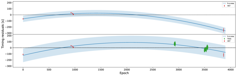
Figure 7: Timing residuals when conducting the TTV modeling of WASP-12 b. Top panel: Quadratic fitting of the HST data alone. Bottom panel: Quadratic fitting of the HST and TESS data together. We obtain $\dot{P}=-31.36\pm 2.95$ ms/yr when fitting the HST data alone, and $\dot{P}=-32.84\pm 1.78$ ms/yr when fitting the HST and TESS data together. For comparison, the original fitting in Section 3.2 with all selected archival data yields $\dot{P}=-30.31\pm 0.85$ ms/yr.

In our study, we often encounter literature timing data reported with unrealistically small error bars, which may not adequately account for all sources of uncertainties from observations, especially from the ground-based telescopes. To demonstrate the significance of using only data with reliable error bars (those with well-known systematics) in the TTV study, we present one such study using WASP-12 b as an example (also see WASP-121 b). We fit a quadratic model using space-based timing data from HST and TESS observations, and show the results in Figure 7. We consider these data as data with the most trustworthy error bars reported. Using only six data points from HST, we obtain a fitting result of $\dot{P}$ as $-31.36\pm 2.95$ ms/yr, compared to $-30.31\pm 0.85$ ms/yr when using all 190 data points from literature data. When using only HST and TESS data, we obtain an orbital period change rate of $-32.84\pm 1.78$ ms/yr. Our findings suggest that a careful selection of observation data can lead to reliable assessments of TTVs of exoplanetary systems. To address this issue, we recommend that future transit exoplanet studies should adopt a more cautious approach when reporting error bars for the timing data, and publish the Monte Carlo chain data generated during the light curve fitting together with the light curve data. Specifically, researchers should consider the potential impact of incomplete transit coverage and other observational limitations, ensuring that the reported uncertainties reflect a realistic assessment of the observational uncertainties. By using more strict standards on error bar reporting, we can enhance the robustness of TTV studies and facilitate comparisons of results from different observational datasets. This practice will ultimately contribute to a deeper understanding of the dynamical properties of short period exoplanet systems.

6 Conclusion

In this study, we analyzed transit observations of 37 exoplanets using HST/WFC3 data. By incorporating these high-precision transit times into our linear and quadratic ephemeris models, we identified candidates exhibiting both long- and short-term orbital period variations. Specifically, we classified six planetary systems as long-term orbital period variation candidates, four as short-term variation candidates, and eight as ‘interesting’ candidates that warrant further observational study. For many known exoplanets, the uncertainty of their predicted transit windows prohibits an accurate scheduling of follow-up observations. Thus we also refined the orbital ephemerides of these planets, which will aid in the planning of future observations. Our results demonstrate the importance of high-precision timing data in improving measurements of planetary orbital period change rates. Our analysis finds strong evidence for orbital period decay in two hot Jupiters. Among the roughly 400 known HJs, several appear to have relatively short inspiral timescales. Given the older ages of their host stars, this may suggest a continuous depletion of HJs and thus the need for HJ replenishment to sustain the observed population. These results support the need of a ‘late-arrived’ hot Jupiter population, as proposed by Chen et al. (2023), which is likely coming through the secular dynamical chaos process (Wu & Lithwick, 2011; Hamers et al., 2017; Teyssandier et al., 2019). In the future, we plan to extend this study by incorporating additional space-based transit observation data from JWST (Gardner et al., 2023), ET2.0 (Ge et al., 2024), PLATO (Rauer et al., 2014), and others. This will allow for more precise estimates of the orbital decay parameter, benefiting from a longer time baseline. The current study can also be applied to the field of short-period transiting brown dwarfs. By investigating the evolution of close brown dwarf companions around solar-type stars, we aim to gain a deeper understanding of the origin of the ‘brown dwarf desert’ (Marcy & Butler, 2000; Halbwachs et al., 2000; Grether & Lineweaver, 2006; Ma & Ge, 2014). Furthermore, the HST data presented in this work, when combined with radial velocity data and TTV analysis, can be used to place constraints on potential hidden planets within the system—an important topic in the exoplanet photodynamics research field.

Appendix A Appendix A

In this section, we show the transit timing data fitting results for all targets showing a constant orbital period trend in our sample, in Figure A1 and  A2.

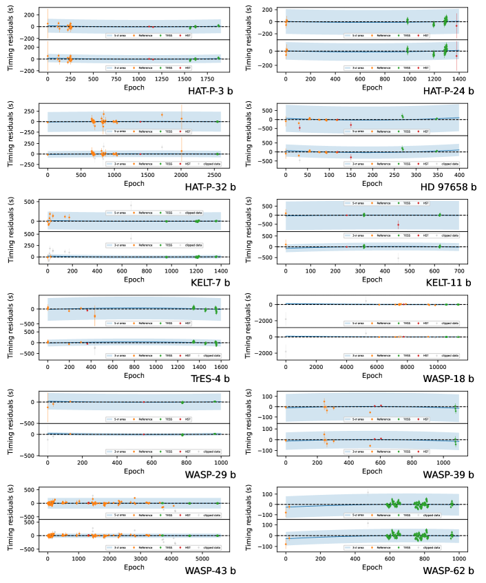
Figure A1: Quadratic TTV model fitting results of all exoplanets in our sample that show an orbital period variation trend consistent with a constant period.

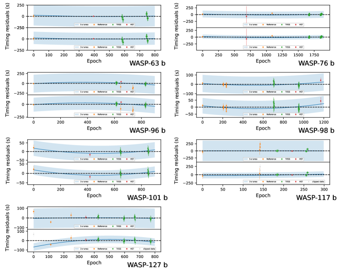
Figure A2: (continued) Quadratic TTV model fitting results of all exoplanets in our sample that show an orbital period variation trend consistent with a constant period.

Appendix B Appendix B

Previous literature references for the data used by the 37 exoplanets in this article: WASP-12 b Hebb et al. (2009); Chan et al. (2011); Sada et al. (2012); Cowan et al. (2012); Copperwheat et al. (2013); Stevenson et al. (2014); Kreidberg et al. (2015); Maciejewski et al. (2016b); Collins et al. (2017); Patra et al. (2017, 2020); Wang et al. (2024) WASP-4 b Wilson et al. (2008); Gillon et al. (2009b); Winn et al. (2009); Dragomir et al. (2011); Sanchis-Ojeda et al. (2011); Nikolov et al. (2012); Hoyer et al. (2013); Ranjan et al. (2014); Huitson et al. (2017); Southworth et al. (2019); Baluev et al. (2019); Bouma et al. (2020); Wang et al. (2024) WASP-80 b Triaud et al. (2013); Mancini et al. (2014); Fukui et al. (2014); Sedaghati et al. (2017); Turner et al. (2017); Wang et al. (2021, 2024) WASP-19 b Hebb et al. (2010); Hellier et al. (2011a); Dragomir et al. (2011); Lendl et al. (2013); Tregloan-Reed et al. (2013); Mancini et al. (2013); Espinoza et al. (2019); Petrucci et al. (2020); Wang et al. (2024) WASP-17 b Anderson et al. (2010, 2011); Southworth et al. (2012); Bento et al. (2014); Sedaghati et al. (2016); Wang et al. (2024) HAT-P-38 b Mallonn et al. (2019); Sato et al. (2012); Bruno et al. (2018); Wang et al. (2024) HAT-P-2 b Pál et al. (2010); Lewis et al. (2013); Wang et al. (2024) HAT-P-11 b Bakos et al. (2010); Murgas et al. (2019); Wang et al. (2024) HAT-P-18 b Seeliger et al. (2015); Wang et al. (2024) WASP-178 b Rodríguez Martínez et al. (2020); Hellier et al. (2019); Wang et al. (2024) WASP-6 b Gillon et al. (2009a); Dragomir et al. (2011); Sada et al. (2012); Jordán et al. (2013); Nikolov et al. (2015); Tregloan-Reed et al. (2015); Wang et al. (2024) HAT-P-26 b Hartman et al. (2011b); Stevenson et al. (2016); Wakeford et al. (2017b); von Essen et al. (2019); Wang et al. (2024) HAT-P-41 b Hartman et al. (2012); Wakeford et al. (2020); Wang et al. (2024) WASP-69 b Baştürk et al. (2019); Wang et al. (2024) HAT-P-17 b Howard et al. (2012); Wang et al. (2024) WASP-79 b Smalley et al. (2012); Brown et al. (2017); Wang et al. (2024) WASP-121 b Delrez et al. (2016); Evans et al. (2018); Wang et al. (2024) HAT-P-12 b Hartman et al. (2009); Lee et al. (2012); Sada et al. (2012); Mallonn et al. (2015); Turner et al. (2017); Mancini et al. (2018); Alexoudi et al. (2018); Sariya et al. (2021); Wang et al. (2024) HAT-P-3 b Torres et al. (2007); Gibson et al. (2010); Chan et al. (2011); Wang et al. (2024) HAT-P-24 b Kipping et al. (2010); Wang et al. (2024) HAT-P-32 b Hartman et al. (2011c); Gibson et al. (2013b); Seeliger et al. (2014); Zellem et al. (2020); Wang et al. (2024) HD 97658 b Dragomir et al. (2013); Guo et al. (2020); Wang et al. (2024) KELT-7 b Bieryla et al. (2015); Wang et al. (2024) KELT-11 b Pepper et al. (2017); Wang et al. (2024) TrES-4 b Mandushev et al. (2007); Sozzetti et al. (2009); Chan et al. (2011); Turner et al. (2016); Wang et al. (2024) WASP-18 b Hellier et al. (2009); Maxted et al. (2013); Wilkins et al. (2017); McDonald & Kerins (2018); Patra et al. (2020); Wang et al. (2024) WASP-29 b Hellier et al. (2010); Dragomir et al. (2011); Gibson et al. (2013a); Bonomo et al. (2017); Wang et al. (2024) WASP-39 b Faedi et al. (2011); Fischer et al. (2016); Kirk et al. (2019); Wang et al. (2024) WASP-43 b Gillon et al. (2012); Murgas et al. (2014); Chen et al. (2014); Stevenson et al. (2014); Ricci et al. (2015); Jiang et al. (2016); Hoyer et al. (2016); Stevenson et al. (2017); Patra et al. (2020); Wang et al. (2021); Garai et al. (2021); Saha et al. (2021); Wang et al. (2024) WASP-62 b Hellier et al. (2012); Brown et al. (2017); Skaf et al. (2020); Garhart et al. (2020); Wang et al. (2024) WASP-63 b Hellier et al. (2012); Wang et al. (2024) WASP-76 b West et al. (2016); Ehrenreich et al. (2020); Wang et al. (2024) WASP-96 b Hellier et al. (2014); Yip et al. (2021); Wang et al. (2024) WASP-98 b Hellier et al. (2014); Mancini et al. (2016); Wang et al. (2024) WASP-101 b Hellier et al. (2014); Wang et al. (2024) WASP-117 b Lendl et al. (2014); Mallonn et al. (2019); Anisman et al. (2020); Wang et al. (2024) WASP-127 b Lam et al. (2017); Palle et al. (2017); Seidel et al. (2020); Skaf et al. (2020); Wang et al. (2024)

References

- A-thano et al. (2023) A-thano, N., Awiphan, S., Jiang, I.-G., et al. 2023, AJ, 166, 223
- Agol et al. (2005) Agol, E., Steffen, J., Sari, R., & Clarkson, W. 2005, Monthly Notices of the Royal Astronomical Society, 359, 567
- Alexoudi et al. (2018) Alexoudi, X., Mallonn, M., von Essen, C., et al. 2018, A&A, 620, A142
- Alvarado et al. (2024) Alvarado, E., Bostow, K. B., Patra, K. C., et al. 2024, MNRAS, 534, 800
- Anderson et al. (2010) Anderson, D. R., Hellier, C., Gillon, M., et al. 2010, ApJ, 709, 159
- Anderson et al. (2011) Anderson, D. R., Smith, A. M. S., Lanotte, A. A., et al. 2011, MNRAS, 416, 2108
- Anderson et al. (2014) Anderson, D. R., Collier Cameron, A., Delrez, L., et al. 2014, MNRAS, 445, 1114
- Anisman et al. (2020) Anisman, L. O., Edwards, B., Changeat, Q., et al. 2020, AJ, 160, 233
- Applegate (1992) Applegate, J. H. 1992, ApJ, 385, 621
- Astropy Collaboration et al. (2013) Astropy Collaboration, Robitaille, T. P., Tollerud, E. J., et al. 2013, A&A, 558, A33
- Astropy Collaboration et al. (2018) Astropy Collaboration, Price-Whelan, A. M., Sipőcz, B. M., et al. 2018, AJ, 156, 123
- Astropy Collaboration et al. (2022) Astropy Collaboration, Price-Whelan, A. M., Lim, P. L., et al. 2022, ApJ, 935, 167
- Baştürk et al. (2019) Baştürk, Ö., Esmer, E. M., Torun, Ş., et al. 2019, in American Institute of Physics Conference Series, Vol. 2178, Turkish Physical Society 35th International Physics Congress (TPS35) (AIP), 030019
- Bai et al. (2022) Bai, L., Gu, S., Wang, X., et al. 2022, Monthly Notices of the Royal Astronomical Society, 512, 3113
- Bailey & Goodman (2019) Bailey, A., & Goodman, J. 2019, MNRAS, 482, 1872
- Bakos et al. (2007) Bakos, G. Á., Kovács, G., Torres, G., et al. 2007, ApJ, 670, 826
- Bakos et al. (2010) Bakos, G. Á., Torres, G., Pál, A., et al. 2010, ApJ, 710, 1724
- Baluev et al. (2019) Baluev, R. V., Sokov, E. N., Jones, H. R. A., et al. 2019, MNRAS, 490, 1294
- Barker (2020) Barker, A. J. 2020, MNRAS, 498, 2270
- Beatty et al. (2017) Beatty, T. G., Stevens, D. J., Collins, K. A., et al. 2017, AJ, 154, 25
- Bento et al. (2014) Bento, J., Wheatley, P. J., Copperwheat, C. M., et al. 2014, MNRAS, 437, 1511
- Bieryla et al. (2015) Bieryla, A., Collins, K., Beatty, T. G., et al. 2015, AJ, 150, 12
- Bonomo et al. (2017) Bonomo, A. S., Desidera, S., Benatti, S., et al. 2017, A&A, 602, A107
- Bouma et al. (2020) Bouma, L. G., Winn, J. N., Howard, A. W., et al. 2020, ApJ, 893, L29
- Bouma et al. (2019) Bouma, L. G., Winn, J. N., Baxter, C., et al. 2019, AJ, 157, 217
- Bourrier et al. (2020) Bourrier, V., Ehrenreich, D., Lendl, M., et al. 2020, A&A, 635, A205
- Brown et al. (2017) Brown, D. J. A., Triaud, A. H. M. J., Doyle, A. P., et al. 2017, MNRAS, 464, 810
- Bruno et al. (2018) Bruno, G., Lewis, N. K., Stevenson, K. B., et al. 2018, AJ, 155, 55
- Casasayas-Barris et al. (2017) Casasayas-Barris, N., Palle, E., Nowak, G., et al. 2017, A&A, 608, A135
- Chan et al. (2011) Chan, T., Ingemyr, M., Winn, J. N., et al. 2011, AJ, 141, 179
- Chatterjee et al. (2008) Chatterjee, S., Ford, E. B., Matsumura, S., & Rasio, F. A. 2008, ApJ, 686, 580
- Chen et al. (2023) Chen, D.-C., Xie, J.-W., Zhou, J.-L., et al. 2023, Proceedings of the National Academy of Science, 120, e2304179120
- Chen et al. (2014) Chen, G., van Boekel, R., Wang, H., et al. 2014, A&A, 563, A40
- Claret (2000) Claret, A. 2000, A&A, 363, 1081
- Collins et al. (2017) Collins, K. A., Kielkopf, J. F., & Stassun, K. G. 2017, AJ, 153, 78
- Copperwheat et al. (2013) Copperwheat, C. M., Wheatley, P. J., Southworth, J., et al. 2013, MNRAS, 434, 661
- Cornachione et al. (2019) Cornachione, M. A., Bolton, A. S., Eastman, J. D., et al. 2019, PASP, 131, 124503
- Cowan et al. (2012) Cowan, N. B., Machalek, P., Croll, B., et al. 2012, ApJ, 747, 82
- Davoudi et al. (2021) Davoudi, F., Baştürk, Ö., Yalçınkaya, S., Esmer, E. M., & Safari, H. 2021, AJ, 162, 210
- Dawson & Johnson (2018) Dawson, R. I., & Johnson, J. A. 2018, ARA&A, 56, 175
- de Beurs et al. (2023) de Beurs, Z. L., de Wit, J., Venner, A., et al. 2023, AJ, 166, 136
- Deck & Agol (2015) Deck, K. M., & Agol, E. 2015, The Astrophysical Journal, 802, 116
- Delrez et al. (2016) Delrez, L., Santerne, A., Almenara, J. M., et al. 2016, MNRAS, 458, 4025
- Dragomir et al. (2011) Dragomir, D., Kane, S. R., Pilyavsky, G., et al. 2011, AJ, 142, 115
- Dragomir et al. (2013) Dragomir, D., Matthews, J. M., Eastman, J. D., et al. 2013, ApJ, 772, L2
- Ehrenreich et al. (2020) Ehrenreich, D., Lovis, C., Allart, R., et al. 2020, Nature, 580, 597
- Ellis et al. (2021) Ellis, T. G., Boyajian, T., von Braun, K., et al. 2021, AJ, 162, 118
- Espinoza et al. (2019) Espinoza, N., Rackham, B. V., Jordán, A., et al. 2019, MNRAS, 482, 2065
- Esposito et al. (2014) Esposito, M., Covino, E., Mancini, L., et al. 2014, A&A, 564, L13
- Esposito et al. (2017) Esposito, M., Covino, E., Desidera, S., et al. 2017, A&A, 601, A53
- Evans et al. (2016) Evans, T. M., Sing, D. K., Wakeford, H. R., et al. 2016, ApJ, 822, L4
- Evans et al. (2018) Evans, T. M., Sing, D. K., Goyal, J. M., et al. 2018, AJ, 156, 283
- Faedi et al. (2011) Faedi, F., Barros, S. C. C., Anderson, D. R., et al. 2011, A&A, 531, A40
- Fang et al. (2023) Fang, Y., Ma, B., Chen, C., & Wen, Y. 2023, Universe, 9, 192
- Fischer et al. (2016) Fischer, P. D., Knutson, H. A., Sing, D. K., et al. 2016, ApJ, 827, 19
- Foreman-Mackey et al. (2013) Foreman-Mackey, D., Hogg, D. W., Lang, D., & Goodman, J. 2013, PASP, 125, 306
- Fukui et al. (2014) Fukui, A., Kawashima, Y., Ikoma, M., et al. 2014, ApJ, 790, 108
- Garai et al. (2021) Garai, Z., Pribulla, T., Parviainen, H., et al. 2021, MNRAS, 508, 5514
- Gardner et al. (2023) Gardner, J. P., Mather, J. C., Abbott, R., et al. 2023, PASP, 135, 068001
- Garhart et al. (2020) Garhart, E., Deming, D., Mandell, A., et al. 2020, AJ, 159, 137
- Ge et al. (2024) Ge, J., Chen, W., Chen, Y., et al. 2024, Chinese Journal of Space Science, 44, 400
- Ghezzi et al. (2018) Ghezzi, L., Montet, B. T., & Johnson, J. A. 2018, ApJ, 860, 109
- Gibson et al. (2013a) Gibson, N. P., Aigrain, S., Barstow, J. K., et al. 2013a, MNRAS, 428, 3680
- Gibson et al. (2013b) —. 2013b, MNRAS, 436, 2974
- Gibson et al. (2010) Gibson, N. P., Pollacco, D. L., Barros, S., et al. 2010, MNRAS, 401, 1917
- Gillon et al. (2009a) Gillon, M., Anderson, D. R., Triaud, A. H. M. J., et al. 2009a, A&A, 501, 785
- Gillon et al. (2009b) Gillon, M., Smalley, B., Hebb, L., et al. 2009b, A&A, 496, 259
- Gillon et al. (2012) Gillon, M., Triaud, A. H. M. J., Fortney, J. J., et al. 2012, A&A, 542, A4
- Goodman & Weare (2010) Goodman, J., & Weare, J. 2010, Communications in Applied Mathematics and Computational Science, 5, 65
- Grether & Lineweaver (2006) Grether, D., & Lineweaver, C. H. 2006, ApJ, 640, 1051
- Guo et al. (2020) Guo, X., Crossfield, I. J. M., Dragomir, D., et al. 2020, AJ, 159, 239
- Hadden & Lithwick (2017) Hadden, S., & Lithwick, Y. 2017, AJ, 154, 5
- Halbwachs et al. (2000) Halbwachs, J. L., Arenou, F., Mayor, M., Udry, S., & Queloz, D. 2000, A&A, 355, 581
- Hamer & Schlaufman (2022) Hamer, J. H., & Schlaufman, K. C. 2022, AJ, 164, 26
- Hamers et al. (2017) Hamers, A. S., Antonini, F., Lithwick, Y., Perets, H. B., & Portegies Zwart, S. F. 2017, MNRAS, 464, 688
- Harre & Smith (2023) Harre, J.-V., & Smith, A. M. S. 2023, Universe, 9, 506
- Hartman et al. (2009) Hartman, J. D., Bakos, G. Á., Torres, G., et al. 2009, ApJ, 706, 785
- Hartman et al. (2011a) Hartman, J. D., Bakos, G. Á., Sato, B., et al. 2011a, ApJ, 726, 52
- Hartman et al. (2011b) Hartman, J. D., Bakos, G. Á., Kipping, D. M., et al. 2011b, ApJ, 728, 138
- Hartman et al. (2011c) Hartman, J. D., Bakos, G. Á., Torres, G., et al. 2011c, ApJ, 742, 59
- Hartman et al. (2012) Hartman, J. D., Bakos, G. Á., Béky, B., et al. 2012, AJ, 144, 139
- Hebb et al. (2009) Hebb, L., Collier-Cameron, A., Loeillet, B., et al. 2009, ApJ, 693, 1920
- Hebb et al. (2010) Hebb, L., Collier-Cameron, A., Triaud, A. H. M. J., et al. 2010, ApJ, 708, 224
- Hellier et al. (2011a) Hellier, C., Anderson, D. R., Collier-Cameron, A., et al. 2011a, ApJ, 730, L31
- Hellier et al. (2009) Hellier, C., Anderson, D. R., Collier Cameron, A., et al. 2009, Nature, 460, 1098
- Hellier et al. (2010) —. 2010, ApJ, 723, L60
- Hellier et al. (2011b) —. 2011b, A&A, 535, L7
- Hellier et al. (2012) —. 2012, MNRAS, 426, 739
- Hellier et al. (2014) —. 2014, MNRAS, 440, 1982
- Hellier et al. (2019) Hellier, C., Anderson, D. R., Barkaoui, K., et al. 2019, MNRAS, 490, 1479
- Holczer et al. (2016) Holczer, T., Mazeh, T., Nachmani, G., et al. 2016, ApJS, 225, 9
- Holman & Murray (2005) Holman, M. J., & Murray, N. W. 2005, Science, 307, 1288
- Horne (1986) Horne, K. 1986, PASP, 98, 609
- Howard et al. (2011) Howard, A. W., Johnson, J. A., Marcy, G. W., et al. 2011, ApJ, 730, 10
- Howard et al. (2012) Howard, A. W., Bakos, G. Á., Hartman, J., et al. 2012, ApJ, 749, 134
- Howarth (2011) Howarth, I. D. 2011, MNRAS, 413, 1515
- Hoyer et al. (2016) Hoyer, S., Pallé, E., Dragomir, D., & Murgas, F. 2016, AJ, 151, 137
- Hoyer et al. (2013) Hoyer, S., López-Morales, M., Rojo, P., et al. 2013, MNRAS, 434, 46
- Huitson et al. (2017) Huitson, C. M., Désert, J. M., Bean, J. L., et al. 2017, AJ, 154, 95
- Hunter (2007) Hunter, J. D. 2007, Computing in Science and Engineering, 9, 90
- Ivshina & Winn (2022) Ivshina, E. S., & Winn, J. N. 2022, ApJS, 259, 62
- Jacobs et al. (2024) Jacobs, B., Désert, J.-M., Lewis, N., et al. 2024, arXiv e-prints, arXiv:2410.11643
- Jiang et al. (2016) Jiang, I.-G., Lai, C.-Y., Savushkin, A., et al. 2016, AJ, 151, 17
- Jontof-Hutter et al. (2015) Jontof-Hutter, D., Rowe, J. F., Lissauer, J. J., Fabrycky, D. C., & Ford, E. B. 2015, Nature, 522, 321
- Jordán et al. (2013) Jordán, A., Espinoza, N., Rabus, M., et al. 2013, ApJ, 778, 184
- Kane et al. (2019) Kane, M., Ragozzine, D., Flowers, X., et al. 2019, AJ, 157, 171
- Kass & Raftery (1995) Kass, R. E., & Raftery, A. E. 1995, Journal of the American Statistical Association, 90, 773
- Kipping et al. (2010) Kipping, D. M., Bakos, G. Á., Hartman, J., et al. 2010, ApJ, 725, 2017
- Kirk et al. (2019) Kirk, J., López-Morales, M., Wheatley, P. J., et al. 2019, AJ, 158, 144
- Kirk et al. (2017) Kirk, J., Wheatley, P. J., Louden, T., et al. 2017, MNRAS, 468, 3907
- Knutson et al. (2014a) Knutson, H. A., Fulton, B. J., Montet, B. T., et al. 2014a, ApJ, 785, 126
- Knutson et al. (2014b) Knutson, H. A., Dragomir, D., Kreidberg, L., et al. 2014b, ApJ, 794, 155
- Kokori et al. (2022) Kokori, A., Tsiaras, A., Edwards, B., et al. 2022, ApJS, 258, 40
- Kokori et al. (2023) —. 2023, ApJS, 265, 4
- Kreidberg (2015) Kreidberg, L. 2015, PASP, 127, 1161
- Kreidberg et al. (2014) Kreidberg, L., Bean, J. L., Désert, J.-M., et al. 2014, Nature, 505, 69
- Kreidberg et al. (2015) Kreidberg, L., Line, M. R., Bean, J. L., et al. 2015, ApJ, 814, 66
- Lai (2012) Lai, D. 2012, MNRAS, 423, 486
- Lam et al. (2017) Lam, K. W. F., Faedi, F., Brown, D. J. A., et al. 2017, A&A, 599, A3
- Lee et al. (2012) Lee, J. W., Youn, J.-H., Kim, S.-L., Lee, C.-U., & Hinse, T. C. 2012, AJ, 143, 95
- Lendl et al. (2013) Lendl, M., Gillon, M., Queloz, D., et al. 2013, A&A, 552, A2
- Lendl et al. (2014) Lendl, M., Triaud, A. H. M. J., Anderson, D. R., et al. 2014, A&A, 568, A81
- Levine et al. (2024) Levine, W. G., Vissapragada, S., Feinstein, A. D., et al. 2024, AJ, 168, 65
- Lewis et al. (2013) Lewis, N. K., Knutson, H. A., Showman, A. P., et al. 2013, ApJ, 766, 95
- Line et al. (2016) Line, M. R., Stevenson, K. B., Bean, J., et al. 2016, AJ, 152, 203
- Loeillet et al. (2008) Loeillet, B., Shporer, A., Bouchy, F., et al. 2008, A&A, 481, 529
- Lu et al. (2024) Lu, T., An, Q., Brandt, G., Li, G., & Brandt, T. 2024, in AAS/Division for Extreme Solar Systems Abstracts, Vol. 56, AAS/Division for Extreme Solar Systems Abstracts, 616.04
- Ma & Ge (2014) Ma, B., & Ge, J. 2014, MNRAS, 439, 2781
- Ma & Ge (2019) —. 2019, MNRAS, 484, 760
- MacDonald & Madhusudhan (2019) MacDonald, R. J., & Madhusudhan, N. 2019, MNRAS, 486, 1292
- Maciejewski et al. (2020) Maciejewski, G., Knutson, H. A., Howard, A. W., et al. 2020, Acta Astron., 70, 1
- Maciejewski et al. (2016a) Maciejewski, G., Dimitrov, D., Mancini, L., et al. 2016a, Acta Astron., 66, 55
- Maciejewski et al. (2016b) Maciejewski, G., Dimitrov, D., Fernández, M., et al. 2016b, A&A, 588, L6
- Mallonn et al. (2015) Mallonn, M., Nascimbeni, V., Weingrill, J., et al. 2015, A&A, 583, A138
- Mallonn et al. (2019) Mallonn, M., von Essen, C., Herrero, E., et al. 2019, A&A, 622, A81
- Mancini et al. (2016) Mancini, L., Giordano, M., Mollière, P., et al. 2016, MNRAS, 461, 1053
- Mancini et al. (2013) Mancini, L., Ciceri, S., Chen, G., et al. 2013, MNRAS, 436, 2
- Mancini et al. (2014) Mancini, L., Southworth, J., Ciceri, S., et al. 2014, A&A, 562, A126
- Mancini et al. (2018) Mancini, L., Esposito, M., Covino, E., et al. 2018, A&A, 613, A41
- Mandel & Agol (2002) Mandel, K., & Agol, E. 2002, ApJ, 580, L171
- Mandushev et al. (2007) Mandushev, G., O’Donovan, F. T., Charbonneau, D., et al. 2007, ApJ, 667, L195
- Marcy & Butler (2000) Marcy, G. W., & Butler, R. P. 2000, PASP, 112, 137
- Maxted et al. (2013) Maxted, P. F. L., Anderson, D. R., Doyle, A. P., et al. 2013, MNRAS, 428, 2645
- Mazeh et al. (2013) Mazeh, T., Nachmani, G., Holczer, T., et al. 2013, ApJS, 208, 16
- McDonald & Kerins (2018) McDonald, I., & Kerins, E. 2018, MNRAS, 477, L21
- McGruder et al. (2023) McGruder, C. D., López-Morales, M., Brahm, R., & Jordán, A. 2023, ApJ, 944, L56
- Ment et al. (2018) Ment, K., Fischer, D. A., Bakos, G., Howard, A. W., & Isaacson, H. 2018, AJ, 156, 213
- Morello et al. (2020) Morello, G., Claret, A., Martin-Lagarde, M., et al. 2020, AJ, 159, 75
- Murgas et al. (2019) Murgas, F., Chen, G., Pallé, E., Nortmann, L., & Nowak, G. 2019, A&A, 622, A172
- Murgas et al. (2014) Murgas, F., Pallé, E., Zapatero Osorio, M. R., et al. 2014, A&A, 563, A41
- Naoz et al. (2012) Naoz, S., Farr, W. M., & Rasio, F. A. 2012, ApJ, 754, L36
- Nesvorný & Morbidelli (2008) Nesvorný, D., & Morbidelli, A. 2008, ApJ, 688, 636
- Nikolov et al. (2012) Nikolov, N., Henning, T., Koppenhoefer, J., et al. 2012, A&A, 539, A159
- Nikolov et al. (2015) Nikolov, N., Sing, D. K., Burrows, A. S., et al. 2015, MNRAS, 447, 463
- Oliphant (2006) Oliphant, T. E. 2006, Guide to NumPy (USA: Trelgol Publishing), available online at the Internet Archive. https://archive.org/details/NumPyBook
- Pál et al. (2010) Pál, A., Bakos, G. Á., Torres, G., et al. 2010, MNRAS, 401, 2665
- Palle et al. (2017) Palle, E., Chen, G., Prieto-Arranz, J., et al. 2017, A&A, 602, L15
- Parviainen (2015) Parviainen, H. 2015, MNRAS, 450, 3233
- Patra et al. (2017) Patra, K. C., Winn, J. N., Holman, M. J., et al. 2017, AJ, 154, 4
- Patra et al. (2020) —. 2020, AJ, 159, 150
- Pepper et al. (2017) Pepper, J., Rodriguez, J. E., Collins, K. A., et al. 2017, AJ, 153, 215
- Petrovich (2015) Petrovich, C. 2015, ApJ, 799, 27
- Petrucci et al. (2020) Petrucci, R., Jofré, E., Gómez Maqueo Chew, Y., et al. 2020, MNRAS, 491, 1243
- Petrucci et al. (2013) Petrucci, R., Jofré, E., Schwartz, M., et al. 2013, ApJ, 779, L23
- Piskunov & Valenti (2002) Piskunov, N. E., & Valenti, J. A. 2002, A&A, 385, 1095
- Ranjan et al. (2014) Ranjan, S., Charbonneau, D., Désert, J.-M., et al. 2014, ApJ, 785, 148
- Rasio & Ford (1996) Rasio, F. A., & Ford, E. B. 1996, Science, 274, 954
- Rauer et al. (2014) Rauer, H., Catala, C., Aerts, C., et al. 2014, Experimental Astronomy, 38, 249
- Ricci et al. (2015) Ricci, D., Ramón-Fox, F. G., Ayala-Loera, C., et al. 2015, PASP, 127, 143
- Ricker (2015) Ricker, G. R. 2015, in AAS/Division for Extreme Solar Systems Abstracts, Vol. 47, AAS/Division for Extreme Solar Systems Abstracts, 503.01
- Rodríguez Martínez et al. (2020) Rodríguez Martínez, R., Gaudi, B. S., Rodriguez, J. E., et al. 2020, AJ, 160, 111
- Rosenthal et al. (2021) Rosenthal, L. J., Fulton, B. J., Hirsch, L. A., et al. 2021, ApJS, 255, 8
- Sada et al. (2012) Sada, P. V., Deming, D., Jennings, D. E., et al. 2012, PASP, 124, 212
- Saha et al. (2021) Saha, S., Chakrabarty, A., & Sengupta, S. 2021, AJ, 162, 18
- Sanchis-Ojeda et al. (2011) Sanchis-Ojeda, R., Winn, J. N., Holman, M. J., et al. 2011, ApJ, 733, 127
- Sariya et al. (2021) Sariya, D. P., Jiang, I.-G., Su, L.-H., et al. 2021, Research in Astronomy and Astrophysics, 21, 097
- Sato et al. (2012) Sato, B., Hartman, J. D., Bakos, G. Á., et al. 2012, PASJ, 64, 97
- Scandariato et al. (2022) Scandariato, G., Singh, V., Kitzmann, D., et al. 2022, A&A, 668, A17
- Schwarz (1978) Schwarz, G. 1978, The annals of statistics, 461
- Sedaghati et al. (2017) Sedaghati, E., Boffin, H. M. J., Delrez, L., et al. 2017, MNRAS, 468, 3123
- Sedaghati et al. (2016) Sedaghati, E., Boffin, H. M. J., Jeřabková, T., et al. 2016, A&A, 596, A47
- Seeliger et al. (2014) Seeliger, M., Dimitrov, D., Kjurkchieva, D., et al. 2014, MNRAS, 441, 304
- Seeliger et al. (2015) Seeliger, M., Kitze, M., Errmann, R., et al. 2015, MNRAS, 451, 4060
- Seidel et al. (2020) Seidel, J. V., Lendl, M., Bourrier, V., et al. 2020, A&A, 643, A45
- Shporer et al. (2019) Shporer, A., Wong, I., Huang, C. X., et al. 2019, AJ, 157, 178
- Skaf et al. (2020) Skaf, N., Bieger, M. F., Edwards, B., et al. 2020, AJ, 160, 109
- Smalley et al. (2012) Smalley, B., Anderson, D. R., Collier-Cameron, A., et al. 2012, A&A, 547, A61
- Southworth et al. (2012) Southworth, J., Hinse, T. C., Dominik, M., et al. 2012, MNRAS, 426, 1338
- Southworth et al. (2019) Southworth, J., Dominik, M., Jørgensen, U. G., et al. 2019, MNRAS, 490, 4230
- Sozzetti et al. (2009) Sozzetti, A., Torres, G., Charbonneau, D., et al. 2009, ApJ, 691, 1145
- Sozzetti et al. (2015) Sozzetti, A., Bonomo, A. S., Biazzo, K., et al. 2015, A&A, 575, L15
- Stevenson et al. (2014) Stevenson, K. B., Bean, J. L., Seifahrt, A., et al. 2014, AJ, 147, 161
- Stevenson et al. (2016) —. 2016, ApJ, 817, 141
- Stevenson et al. (2017) Stevenson, K. B., Line, M. R., Bean, J. L., et al. 2017, AJ, 153, 68
- STScI (2016) STScI. 2016, Hubble Source Catalog, STScI/MAST, doi:10.17909/T97P46. http://archive.stsci.edu/doi/resolve/resolve.html?doi=10.17909/T97P46
- Sun et al. (2017) Sun, L., Gu, S., Wang, X., et al. 2017, The Astronomical Journal, 153, 28
- Teyssandier et al. (2019) Teyssandier, J., Lai, D., & Vick, M. 2019, MNRAS, 486, 2265
- Torres et al. (2008) Torres, G., Winn, J. N., & Holman, M. J. 2008, ApJ, 677, 1324
- Torres et al. (2007) Torres, G., Bakos, G. Á., Kovács, G., et al. 2007, ApJ, 666, L121
- Tregloan-Reed et al. (2013) Tregloan-Reed, J., Southworth, J., & Tappert, C. 2013, MNRAS, 428, 3671
- Tregloan-Reed et al. (2015) Tregloan-Reed, J., Southworth, J., Burgdorf, M., et al. 2015, MNRAS, 450, 1760
- Triaud et al. (2010) Triaud, A. H. M. J., Collier Cameron, A., Queloz, D., et al. 2010, A&A, 524, A25
- Triaud et al. (2013) Triaud, A. H. M. J., Anderson, D. R., Collier Cameron, A., et al. 2013, A&A, 551, A80
- Triaud et al. (2015) Triaud, A. H. M. J., Gillon, M., Ehrenreich, D., et al. 2015, MNRAS, 450, 2279
- Tsiaras et al. (2016a) Tsiaras, A., Waldmann, I. P., Rocchetto, M., et al. 2016a, ApJ, 832, 202
- Tsiaras et al. (2016b) Tsiaras, A., Rocchetto, M., Waldmann, I. P., et al. 2016b, ApJ, 820, 99
- Tsiaras et al. (2018) Tsiaras, A., Waldmann, I. P., Zingales, T., et al. 2018, AJ, 155, 156
- Turner et al. (2022) Turner, J. D., Flagg, L., Ridden-Harper, A., & Jayawardhana, R. 2022, AJ, 163, 281
- Turner et al. (2021) Turner, J. D., Ridden-Harper, A., & Jayawardhana, R. 2021, AJ, 161, 72
- Turner et al. (2016) Turner, J. D., Pearson, K. A., Biddle, L. I., et al. 2016, MNRAS, 459, 789
- Turner et al. (2017) Turner, J. D., Leiter, R. M., Biddle, L. I., et al. 2017, MNRAS, 472, 3871
- Van Grootel et al. (2014) Van Grootel, V., Gillon, M., Valencia, D., et al. 2014, ApJ, 786, 2
- Virtanen et al. (2020) Virtanen, P., Gommers, R., Oliphant, T. E., et al. 2020, Nature Methods, 17, 261
- von Essen et al. (2019) von Essen, C., Wedemeyer, S., Sosa, M. S., et al. 2019, A&A, 628, A116
- Wakeford et al. (2016) Wakeford, H. R., Sing, D. K., Evans, T., Deming, D., & Mandell, A. 2016, ApJ, 819, 10
- Wakeford et al. (2017a) Wakeford, H. R., Stevenson, K. B., Lewis, N. K., et al. 2017a, ApJ, 835, L12
- Wakeford et al. (2017b) Wakeford, H. R., Sing, D. K., Kataria, T., et al. 2017b, Science, 356, 628
- Wakeford et al. (2020) Wakeford, H. R., Sing, D. K., Stevenson, K. B., et al. 2020, AJ, 159, 204
- Wang et al. (2018) Wang, S., Wang, X.-Y., Wang, Y.-H., et al. 2018, AJ, 156, 181
- Wang et al. (2024) Wang, W., Zhang, Z., Chen, Z., et al. 2024, ApJS, 270, 14
- Wang et al. (2021) Wang, X.-Y., Wang, Y.-H., Wang, S., et al. 2021, ApJS, 255, 15
- Wang et al. (2019) Wang, Y.-H., Wang, S., Hinse, T. C., et al. 2019, AJ, 157, 82
- West et al. (2016) West, R. G., Hellier, C., Almenara, J. M., et al. 2016, A&A, 585, A126
- Wilkins et al. (2017) Wilkins, A. N., Delrez, L., Barker, A. J., et al. 2017, ApJ, 836, L24
- Wilson et al. (2008) Wilson, D. M., Gillon, M., Hellier, C., et al. 2008, ApJ, 675, L113
- Winn et al. (2009) Winn, J. N., Holman, M. J., Carter, J. A., et al. 2009, AJ, 137, 3826
- Wong et al. (2016) Wong, I., Knutson, H. A., Kataria, T., et al. 2016, ApJ, 823, 122
- Wu et al. (2023) Wu, D.-H., Rice, M., & Wang, S. 2023, AJ, 165, 171
- Wu & Lithwick (2011) Wu, Y., & Lithwick, Y. 2011, ApJ, 735, 109
- Xie (2013) Xie, J.-W. 2013, ApJS, 208, 22
- Yee et al. (2018) Yee, S. W., Petigura, E. A., Fulton, B. J., et al. 2018, AJ, 155, 255
- Yee et al. (2020) Yee, S. W., Winn, J. N., Knutson, H. A., et al. 2020, ApJ, 888, L5
- Yip et al. (2021) Yip, K. H., Changeat, Q., Edwards, B., et al. 2021, AJ, 161, 4
- Zechmeister et al. (2014) Zechmeister, M., Anglada-Escudé, G., & Reiners, A. 2014, A&A, 561, A59
- Zellem et al. (2020) Zellem, R. T., Pearson, K. A., Ciardi, D., et al. 2020, in American Astronomical Society Meeting Abstracts, Vol. 235, American Astronomical Society Meeting Abstracts #235, 337.07
- Zhang et al. (2024) Zhang, Z., Wang, W., Ma, X., et al. 2024, ApJS, 275, 32
- Zhou et al. (2022) Zhou, L., Ma, B., Wang, Y., & Zhu, Y. 2022, AJ, 164, 203
- Zhou et al. (2023) Zhou, L., Ma, B., Wang, Y.-H., & Zhu, Y.-N. 2023, Research in Astronomy and Astrophysics, 23, 025011
- Zink & Howard (2023) Zink, J. K., & Howard, A. W. 2023, ApJ, 956, L29