Towards optimization of the Josephson diode effect

Abstract

We theoretically study the Josephson diode effect in the junction of singlet superconductors separated by the Rashba system in the in-plane magnetic field perpendicular to the bias current. The coupling energy of two superconductors is formulated under the bias current using a tunneling Hamiltonian with a one-dimensional model. The bias current shifts the Fermi momentum in the Rashba system due to the continuity of the electronic current. Including the shift of Fermi momentum in the coupling energy, it is found that the critical current is asymmetric with respect to the current and the magnetic field, i.e., Josephson diode effect. Depending on a distance between the superconducting electrodes $d$, the Josephson diode effect changes its magnitude and sign. The magnitude is inversely proportional to a band split caused by the spin-orbit interaction. Since $d$ is experimentally controllable, the Josephson diode effect can be optimized by tuning of $d$. Our theory develops a new guiding principle to design the Josephson diode device.

I Introduction

The superconducting diode effect is a phenomenon whereby the superconducting critical current ($I_{c}$) depends on the direction of an applied current in a magnetic field. The asymmetry of $I_{c}$ has been observed in a metal-semiconductor multilayer and is associated with an asymmetric flux flow kadin88 ; broussard88 . The superconducting diode effect has also been reported using a high-$T_{c}$ cuprate/ferromagnetic manganese heterostructure for magnetic memory applications touitou04 . Recently, Ando et al. have reported the superconducting diode effect in the multilayer composed of three elements, i.e., Nb, Ta, and V without an inversion center ando20 ; miyaska21 . They have reported that their superconducting diode effect arises from the magnetochiral anisotropy effect induced by a spin–orbit interaction. This is different from the flux flow mechanism and has inspired many studies of the superconducting diode effect kawarazaki22 ; narita22 ; hou23 . The theoretical studies propose that the superconducting diode effect is caused by the spatial variation of the superconducting order parameter, e.g., helical superconductor, due to the spin-orbit interaction edelstein96 ; daido22 ; he22 ; yuan22 ; aoyama24 .

Motivated by the superconducting diode effect, the non-reciprocity of $I_{c}$ in Josephson junctions is also studied experimentally baumgartner22 ; jeon22 ; pal22 ; wu22 ; kim24 ; ando24 . A typical device consists of two superconducting electrodes coupled via a two dimensional electron system with a spin-orbit interaction, i.e., Rashba system rashba60 ; rashba84 . The current-voltage curve of Josephson junction is measured by applying a current $I_{B}$. When the in-plane magnetic field perpendicular to $I_{B}$ is simultaneously applied to the Rashba system (See Fig. 1 (a)), $I_{c}$ with positive current ($I_{c}^{+}$) is different from $I_{c}$ with negative current ($I_{c}^{-}$), i.e., $I_{c}^{+}\neq I_{c}^{-}$ (See Fig. 1 (b)). The phenomenon is reversed by reversing the direction of the magnetic field. We call it Josephson diode effect instead of the superconducting diode effect.

Theoretically, the Josephson junction via the Rashba system with a magnetic field was studied by Bezuglyi et al. bezuglyi02 , although the Josephson diode effect was not addressed. They reported $I_{c}$ oscillates with the magnetic field or the distance of superconducting electrodes, $d$. This is the same mechanism as the superconductor/ferromagnet/superconductor (SFS) junction bulaevskii77 ; buzdin82 , in which $I_{c}$ changes its sign with $d$ ryazanov01 ; kontos02 ; sellier03 ; frolov04 ; bell05 ; oboznov06 ; shelukhin06 ; robinson06 ; born06 ; weides06 . The negative $I_{c}$ means that the current-phase relation shifted by $\pi$, i.e., the $\pi$-junction bulaevskii77 ; buzdin82 . It is expected to provide various applications for classical digital logic elements and flux-bias-free flux qubit yamashita05 ; yamashita20 . The distance between superconductors essentially changes the transport property of Josephson junction and opens a new pathway for the application.

The Josephson diode effect has been theoretically studied by many authors buzdin08 ; yokoyama14 ; zhang22 ; davydova22 ; souto22 ; tanaka22 ; lu23 ; hu23 ; fu24 ; cayao24 ; debnath24 ; soori24 ; fracasse24 ; yerin24 ; ilic24 ; soori25 ; debnath25 . In those studies, the Josephson diode effect was discussed as the asymmetric current-phase relation due to the spin-orbit interaction in the presence of the Josephson coupling energy involving higher harmonics as a function of the phase. Yokoyama et al. numerically examined the asymmetric current-phase relation and reported the directional dependence of the critical current yokoyama14 . The Andreev bound state is examined to calculate the current phase relation of the junction with a transparent interface davydova22 ; tanaka22 ; lu23 ; hu23 ; fu24 ; cayao24 . The $d$-dependence of the Josephson diode effect was discussed in the references lu23 ; ilic24 . However, the previous studies did not include the bias current explicitly in their formulation. The Josephson diode effect occurs as the response to the bias current. Therefore, including the bias current into the formulation is important to study the Josephson diode effect.

In this paper, we study the Josephson diode effect in the junction of two singlet superconductors separated by the Rashba system with distance $d$. The coupling energy of two superconductors is formulated under the bias current using a tunneling Hamiltonian with a one-dimensional model. The bias current is of crucial importance for the Josephson diode effect. In the Rashba system, the bias current is described by shift of the Fermi momentum due to the continuity of the electronic current. By including the bias current in the formulation, the first harmonic of the Josephson coupling reproduces the Josephson diode effect. Our analytical results suggest that the magnitude and the sign of $I_{c}^{+}-I_{c}^{-}$ depends on $d$. It will be useful to develop a new guiding principle to design the Josephson diode device.

This paper is organized as follows: Sec. II presents the model and Hamiltonian; Sec. III provides a coupling energy of the junction in the fourth order of tunneling matrix element; Sec. IV, the Josephson diode effect is examined by calculating the coupling energy with the applied current. We show the $d$-dependence of the Josephson diode effect. Sec. V provides a summary. The reduced Planck constant $\hbar$ and the Boltzmann constant $k_{B}$ are taken to be unity.

II Hamiltonian: Linearized one-dimensional model

The Josephson junction separated by the Rashba system is illustrated in Fig. 1 (a). Under the in-plane magnetic field $h_{y}$ perpendicular to $I_{B}$, $I_{c}$ in the positive branch $I_{c}^{+}$ (red) is different from $I_{c}$ in the negative branch $I_{c}^{-}$ (blue) as shown in Fig. 1 (b). The difference between $I_{c}^{+}$ and $I_{c}^{-}$, i.e., $I_{c}^{+}-I_{c}^{-}$, is reversed by reversing $I_{B}$ or $h_{y}$. Therefore, the Josephson diode effect is characterized by $I_{c}^{+}-I_{c}^{-}\propto I_{B}\cdot h_{y}$ note2 . $I_{c}$ of Josephson junction is calculated using the Josephson coupling energy between two superconductors (SCs). The current-phase relation is also derived by taking the derivative of the coupling energy with respect to the phase difference of two SCs.

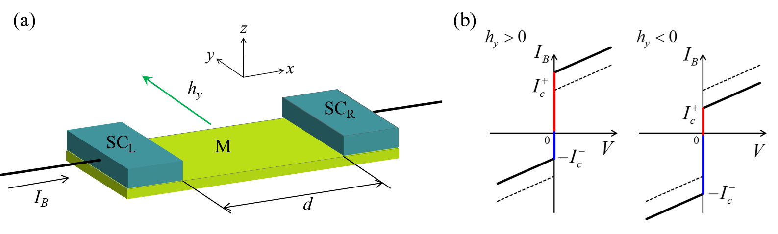
Figure 1: (a) The device geometry of the Josephson junction through the Rashba system (M). The two SCs (SC_R and SC_L) are separated by the Rashba system with distance $d$. An external magnetic field $h_{y}$ is applied in the direction perpendicular to the applied current $I_{B}$. The signs of $I_{B}$ and $h_{y}$ are defined by the Cartesian coordinate shown in this panel. (b) The schematics of the current-voltage curve of the Josephson junction. Due to the Josephson diode effect, $I_{c}$ in the positive branch ($I_{c}^{+}$) colored by red is different from that in the negative one ($I_{c}^{-}$) colored by blue. The broken line is the curve without magnetic field, i.e., $h_{y}=0$. For $h_{y}>0$ ($h_{y}<0$), the curve is shifted up (down) from that with $h_{y}=0$. The amount of the shift is reversed by reversing $h_{y}$. The Josephson diode effect is characterized by $I_{c}^{+}-I_{c}^{-}\propto I_{B}\cdot h_{y}$

In order to obtain an analytical formula of the coupling energy, we use a one-dimensional model, in which the dispersion relation of electrons is linearized around the Fermi momentum $\pm k_{F}$.

The Hamiltonian of singlet SC in left (SC_L, $\lambda$ = L) and right (SC_R, $\lambda$ = R) electrode is given by,

$$H_{\lambda} =\sum\limits_{k,\sigma=\pm}\left[v_{F}\left(k-k_{F}\right)a_{\lambda k\sigma}^{\dagger}{a_{\lambda k\sigma}}-v_{F}\left(k+k_{F}\right)b_{\lambda k\sigma}^{\dagger}{b_{\lambda k\sigma}}\right]$$

$$+\sum\limits_{k,\sigma=\pm}\left[v_{F}\left(k+k_{F}\right)a_{\lambda\overline{k}\sigma}a_{\lambda\overline{k}\sigma}^{\dagger}-v_{F}\left(k-k_{F}\right)b_{\lambda\overline{k}\sigma}b_{\lambda\overline{k}\sigma}^{\dagger}\right]$$

$$+\sum\limits_{k,\sigma=\pm}\Bigl{[}\sigma\Delta\left(a_{\lambda k\sigma}^{\dagger}b_{\lambda\overline{k}\overline{\sigma}}^{\dagger}+b_{\lambda k\sigma}^{\dagger}a_{\lambda\overline{k}\overline{\sigma}}^{\dagger}\right)$$

$$\hskip 30.0pt-\sigma\Delta^{*}\Bigl{(}b_{\lambda\overline{k}\overline{\sigma}}a_{\lambda k\sigma}+a_{\lambda\overline{k}\overline{\sigma}}b_{\lambda k\sigma}\Bigr{)}\Bigr{]},$$ (1)

$$\Delta \equiv{\cal I}\langle a_{\lambda k+}b_{\lambda\overline{k}-}-a_{\lambda k-}b_{\lambda\overline{k}+}\rangle,$$ (2)

with momentum $k$ ($\overline{k}$ $\equiv$ $-k$), Fermi velocity $v_{F}$, and electrons spin $\sigma$ ($\overline{\sigma}$ $\equiv$ $-\sigma$). The singlet superconducting state by interaction ${\cal I}$ is assumed in the both electrodes. The electron creation (annihilation) operators around $+k_{F}$ and $-k_{F}$ are denoted by $a_{\lambda k\sigma}^{\dagger}$ and $b_{\lambda k\sigma}^{\dagger}$ ($a_{\lambda k\sigma}$ and $b_{\lambda k\sigma}$), respectively.

In our theory, the Rashba system is introduced by the following one-dimensional model,

$${H_{M}} ={H_{1}}+{H_{2}}+{H_{3}}+{H_{4}}$$ (3)

$${H_{1}} =\sum\limits_{k,\sigma,\sigma^{\prime}}{a_{k\sigma}^{\dagger}\left\{{\left[{{v_{F}}\left({k-{k_{F}}}\right)-{\gamma h_{z}}{\tau_{3\sigma\sigma^{\prime}}}}\right]-\left({\alpha_{R}{k_{F}}-{\gamma h_{y}}}\right){\tau_{2\sigma\sigma^{\prime}}}}\right\}{a_{k\sigma^{\prime}}}}$$ (4)

$${H_{2}} =\sum\limits_{k,\sigma,\sigma^{\prime}}{b_{k\sigma}^{\dagger}\left\{{\left[{-{v_{F}}\left({k+{k_{F}}}\right)-{\gamma h_{z}}{\tau_{3\sigma\sigma^{\prime}}}}\right]+\left({\alpha_{R}{k_{F}}+{\gamma h_{y}}}\right){\tau_{2\sigma\sigma^{\prime}}}}\right\}{b_{k\sigma^{\prime}}}}$$ (5)

$${H_{3}} =\sum\limits_{k,\sigma,\sigma^{\prime}}{{a_{\overline{k}\sigma}}\left\{{\left[{{v_{F}}\left({k+{k_{F}}}\right)+{\gamma h_{z}}{\tau_{3\sigma\sigma^{\prime}}}}\right]+\left({\alpha_{R}{k_{F}}-{\gamma h_{y}}}\right){\tau_{2\sigma\sigma^{\prime}}}}\right\}}a_{\overline{k}\sigma^{\prime}}^{\dagger}$$ (6)

$${H_{4}} =\sum\limits_{k,\sigma,\sigma^{\prime}}{{b_{\overline{k}\sigma}}\left\{{\left[{-{v_{F}}\left({k-{k_{F}}}\right)+{\gamma h_{z}}{\tau_{3\sigma\sigma^{\prime}}}}\right]-\left({\alpha_{R}{k_{F}}+{\gamma h_{y}}}\right){\tau_{2\sigma\sigma^{\prime}}}}\right\}b_{\overline{k}\sigma^{\prime}}^{\dagger}},$$ (7)

with the Pauli matrix $\tau_{n}$ ($n=1,2,3$), external magnetic field in $y$ ($z$) direction $h_{y}$ ($h_{z}$), and a Rashba parameter $\alpha_{R}$ rashba60 ; rashba84 . The parameter $\gamma$ is defined by $\gamma\equiv g\mu_{B}$ with electron $g$-factor $g$ and Bohr magneton $\mu_{B}$. The electron creation (annihilation) operators around $+k_{F}$ and $-k_{F}$ are denoted by $a_{k\sigma}^{\dagger}$ and $b_{k\sigma}^{\dagger}$ ($a_{k\sigma}$ and $b_{k\sigma}$), respectively. A spin configuration on each Fermi point $\pm k_{F}$ depends on a momentum due to the spin-orbit interaction as shown in Fig. 2, in which the solid lines shows the dispersion relation on the right and left going electrons $E_{R}$ and $E_{L}$ given by,

$$E_{R} ={v_{F}}\left({k-{k_{F}}}\right)\pm\left|{{\alpha_{R}}{k_{F}}-\gamma{h_{y}}}\right|,$$ (8)

$$E_{L} =-{v_{F}}\left({k+{k_{F}}}\right)\pm\left|{{\alpha_{R}}{k_{F}}+\gamma{h_{y}}}\right|.$$ (9)

The circles with blue dot and red cross indicate spin direction parallel and anti-parallel to the $y$-direction on each Fermi point, respectively. In the right branch, the blue (red) lines corresponds to the positive (negative) sign of Eq. (8), and in the left branch vice versa with Eq. (9). The dotted broken line shows the dispersion relations without $\alpha_{R}$ nor $h_{y}$. The dotted line is split into a couple of blue and red solid lines by $\alpha_{R}$. The splitting of two bands is given by $2\alpha_{R}k_{F}$ for $h_{y}=0$ (upper panel of Fig. 2).

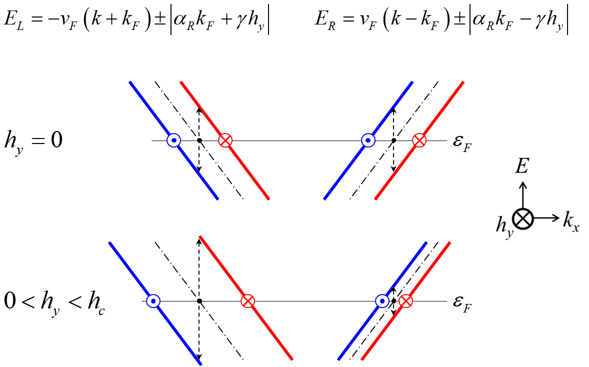
Figure 2: The magnetic field dependence of the Fermi points in one-dimension. The circles with blue dot and red cross indicate spin direction parallel and anti-parallel to the y-direction on each Fermi point, respectively. The horizontal thin line denotes the Fermi energy $\varepsilon_{F}=v_{F}k_{F}$. The upper panel shows the dispersion relation without an in-plane magnetic field $h_{y}$, which is perpendicular to a $x$-direction, and the lower one is for the case of $0<h_{y}<h_{c}$, where $h_{c}\equiv\alpha_{R}k_{F}/\gamma$.

Increasing $h_{y}$, the splittings of the left and right branches become no longer the same as, $2\left|{{\alpha_{R}}{k_{F}}+\gamma{h_{y}}}\right|$ for the left, and $2\left|{{\alpha_{R}}{k_{F}}-\gamma{h_{y}}}\right|$ for the right. In the right branch, the two bands with red and blue merge into one at $h_{y}=\alpha_{R}k_{F}/\gamma\equiv h_{c}$ and split again swapping the spin orientation. It should be noted that physical property will not have singularity around $h_{c}$.

The tunneling Hamiltonian $H_{\rm TL}$ ($H_{\rm TR}$) between SC_L (SC_R) and M is given by,

$$H_{\rm TL} =\hskip-8.0pt\sum\limits_{k,q,\sigma=\pm}\hskip-5.0ptt\left[\bigl{(}a_{L,k\sigma}^{\dagger}+b_{L,k\sigma}^{\dagger}\bigr{)}\bigl{(}a_{q\sigma}+b_{q\sigma}\bigr{)}+H.c.\right]$$

$$-\hskip-8.0pt\sum\limits_{k,q,\sigma=\pm}\hskip-5.0ptt\left[\bigl{(}a_{L,-k\sigma}+b_{L,-k\sigma}\bigr{)}\bigl{(}a_{-q\sigma}^{\dagger}+b_{-q\sigma}^{\dagger}\bigr{)}+H.c.\right],$$ (10)

$${H_{\rm TR}} =\hskip-8.0pt\sum\limits_{k,q,\sigma=\pm}\hskip-5.0ptte^{i(k-q)d}\left[\bigl{(}a_{R,k\sigma}^{\dagger}+b_{R,k\sigma}^{\dagger}\bigr{)}\bigl{(}a_{q\sigma}+b_{q\sigma}\bigr{)}+H.c.\right]$$

$$-\hskip-8.0pt\sum\limits_{k,q,\sigma=\pm}\hskip-5.0ptte^{i(k-q)d}\Bigl{[}\bigl{(}a_{R,-k\sigma}+b_{R,-k\sigma}\bigr{)}\bigl{(}a_{-q\sigma}^{\dagger}+b_{-q\sigma}^{\dagger}\bigr{)}$$

$$\hskip 60.0pt+H.c.\bigr{]},$$ (11)

where the electrode distance between SC_L and SC_R is denoted by $d$. The tunneling matrix element $t$ is assumed to be constant.

III Josephson coupling energy between two superconductors

The Josephson coupling energy $F$ is proportional to $\cos(\phi+\phi_{0})$ with a phase difference of SCs $\phi$ and a constant $\phi_{0}$. $I_{c}$ is estimated by the amplitude of the $\cos\phi$ term. In the fourth order of $t$ (See Fig. 3), $F$ is given by,

$$F =\frac{t^{4}}{4}(\pi\rho_{F})^{2}\sum_{n}\frac{|\Delta|^{2}}{\omega_{n}^{2}+|\Delta|^{2}}\Bigl{[}e^{+i\phi}\sum_{k,k^{\prime}}{\cal A}(k,k^{\prime})e^{+i\left(k-k^{\prime}\right)d}+e^{-i\phi}\sum_{k,k^{\prime}}{\cal A}(k,k^{\prime})e^{-i\left(k-k^{\prime}\right)d}\Bigr{]},$$ (12)

$${\cal A}(k,k^{\prime}) \equiv\sum_{\begin{subarray}{c}m=1,2\\ m^{\prime}=3,4\end{subarray}}\Bigl{\{}g_{m++}({\bm{k}^{\prime}})g_{m^{\prime}--}^{*}(-{\bm{k}})+g_{m--}({\bm{k}^{\prime}})g_{m^{\prime}++}^{*}(-{\bm{k}})-\bigl{[}g_{m-+}({\bm{k}^{\prime}})g_{m^{\prime}-+}^{*}(-{\bm{k}})+g_{m+-}({\bm{k}^{\prime}})g_{m^{\prime}+-}^{*}(-{\bm{k}})\bigr{]}\Bigr{\}}.$$ (13)

with ${\bm{k}}\equiv(k,i\omega_{n})$ and Matsubara frequency of fermion $\omega_{n}$. The prime indicates a different momentum and a different frequency.

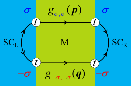
Figure 3: Diagrams contributing to the Josephson coupling. The Josephson diode effect comes from the process of the lower panel

The Greens functions $g_{n\alpha\beta}$ ($n=1-4$ and $\alpha,\beta=+,-$) is given by,

$$\left(\begin{array}[]{cc}g_{1++}({\bm{k}})&g_{1+-}({\bm{k}})\\ g_{1-+}({\bm{k}})&g_{1--}({\bm{k}})\end{array}\right) =\frac{1}{{\left({vp+{\Lambda_{-}}-i\omega_{n}}\right)\left({vp-{\Lambda_{-}}-i\omega_{n}}\right)}}\left({\begin{array}[]{*{20}{c}}{i\omega_{n}-vp-{\gamma h_{z}}}&{+i\lambda_{-}}\\ {-i\lambda_{-}}&{i\omega_{n}-vp+{\gamma h_{z}}}\end{array}}\right),$$ (18)

$$\left(\begin{array}[]{cc}g_{2++}({\bm{k}})&g_{2+-}({\bm{k}})\\ g_{2-+}({\bm{k}})&g_{2--}({\bm{k}})\end{array}\right) =\frac{1}{{\left({vq+{\Lambda_{+}}+i\omega_{n}}\right)\left({vq-{\Lambda_{+}}+i\omega_{n}}\right)}}\left({\begin{array}[]{*{20}{c}}{i\omega_{n}+vq-{\gamma h_{z}}}&{-i\lambda_{+}}\\ {+i\lambda_{+}}&{i\omega_{n}+vq+{\gamma h_{z}}}\end{array}}\right),$$ (23)

$$\left(\begin{array}[]{cc}g_{3++}^{*}(-{\bm{k}})&g_{3+-}^{*}(-{\bm{k}})\\ g_{3-+}^{*}(-{\bm{k}})&g_{3--}^{*}(-{\bm{k}})\end{array}\right) =\frac{1}{{\left({vq+{\Lambda_{-}}-i\omega_{n}}\right)\left({vq-{\Lambda_{-}}-i\omega_{n}}\right)}}\left({\begin{array}[]{*{20}{c}}{i\omega_{n}-vq+{\gamma h_{z}}}&{-i\lambda_{-}}\\ {+i\lambda_{-}}&{i\omega_{n}-vq-{\gamma h_{z}}}\end{array}}\right),$$ (28)

$$\left(\begin{array}[]{cc}g_{4++}^{*}(-{\bm{k}})&g_{4+-}^{*}(-{\bm{k}})\\ g_{4-+}^{*}(-{\bm{k}})&g_{4--}^{*}(-{\bm{k}})\end{array}\right) =\frac{1}{{\left({vp+{\Lambda_{+}}+i\omega_{n}}\right)\left({vp-{\Lambda_{+}}+i\omega_{n}}\right)}}\left({\begin{array}[]{*{20}{c}}{i\omega_{n}+vp+{\gamma h_{z}}}&{i\lambda_{+}}\\ {-i\lambda_{+}}&{i\omega_{n}+vp-{\gamma h_{z}}}\end{array}}\right),$$ (33)

$$\lambda_{-} \equiv\left({\alpha_{R}{k_{F}}-{\gamma h_{y}}}\right),$$ (34)

$$\lambda_{+} \equiv\left({\alpha_{R}{k_{F}}+{\gamma h_{y}}}\right).$$ (35)

$$vp \equiv{v_{F}}\left({k-{k_{F}}}\right),$$ (36)

$$vq \equiv{v_{F}}\left({k+{k_{F}}}\right).$$ (37)

Summing over $k$ and $k^{\prime}$, Eq. (12) is reduced to,

$$F =-t^{4}\,{\cal U}\,{\cal V}\cos\phi,$$ (38)

by which $I_{c}$ is estimated as $t^{4}{\cal U}{\cal V}$. One of prefactors ${\cal U}$ is given by,

$${\cal U} =\left(\frac{2\pi}{v_{F}}\right)^{2}T\sum_{n}\frac{(\pi\rho_{F})^{2}\Delta^{2}}{\omega_{n}^{2}+\Delta^{2}}e^{-2|\omega_{n}|d/v_{F}}\theta(-\omega_{n}),$$ (39)

$$=\left(\frac{2\pi}{v_{F}}\right)^{2}\hskip-3.0pt\frac{(\pi\rho_{F})^{2}}{2\Delta^{2}}\hskip-5.0pt\int_{0}^{\infty}dx\sin x\left[{\rm cosech}\left(\frac{\pi Tx}{\Delta}+\frac{d}{\xi_{T}}\right)\right],$$ (40)

$$\propto\left\{\begin{array}[]{cl}\exp\!\left(-\dfrac{d}{\xi_{T}}\right)&\text{ for $d/\xi_{T}\gg 1$}\\[5.0pt] \dfrac{\xi_{0}}{d}&\text{ for $T\rightarrow 0$}\end{array}\right.,$$ (43)

with $\xi_{T}\equiv v_{F}/2\pi T$ and $\xi_{0}\equiv v_{F}/2\Delta$. Details to derive Eqs. (40) and (43) are given in Ref. mori07 . The factor ${\cal U}$ exponentially decays with $d$ for $d/\xi_{T}\gg 1$ and becomes a power-low decay at low temperatures. The other factor ${\cal V}$, on the other hand, includes the spin-orbit interaction and is given by,

$${\cal V} =\left[{\cos\!\left(\frac{\Lambda_{-}d}{v_{F}}\right)\cos\!\left(\frac{\Lambda_{+}d}{v_{F}}\right)-\frac{(\gamma h_{z})^{2}}{\Lambda_{-}\Lambda_{+}}\sin\!\left(\frac{\Lambda_{-}d}{v_{F}}\right)\sin\!\left(\frac{\Lambda_{+}d}{v_{F}}\right)}\right]+\frac{\lambda_{-}\lambda_{+}}{\Lambda_{-}\Lambda_{+}}\sin\!\left(\frac{\Lambda_{-}d}{v_{F}}\right)\sin\!\left(\frac{\Lambda_{+}d}{v_{F}}\right),$$ (44)

$$\Lambda_{\pm} \equiv\sqrt{(\gamma h_{z})^{2}+{{\left({\alpha_{R}{k_{F}}\pm{\gamma h_{y}}}\right)}^{2}}}.$$ (45)

This factor Eq. (44) essentially changes the transport property of the Josephson junction, because ${\cal V}$ can be negative, i.e., the $\pi$-junction bulaevskii77 ; buzdin82 . In Eq. (44), the first and second terms are the contribution of diagonal part, i.e., $g_{n++}g_{m--}^{*}+g_{n--}g_{m++}^{*}$, and the last term is the result of the off-diagonal part, i.e., $g_{n+-}g_{m-+}^{*}+g_{n-+}g_{m+-}^{*}$, respectively.

For $h_{z}=0$, $h_{y}=0$, and $\alpha_{R}\neq 0$, Eq. (44) becomes constant as,

$${\cal V}=1.$$ (46)

The spin-orbit interaction does not change the coupling between singlet SCs. For $h_{z}\neq 0$, $h_{y}=0$, and $\alpha_{R}=0$, Eq. (44) leads to,

$${\cal V}=\cos\!\left(\frac{2\gamma h_{z}d}{v_{F}}\right),$$ (47)

which reproduces the case of the SC/ferromagnet/SC (SFS) junction bulaevskii77 ; buzdin82 ; ryazanov01 ; kontos02 ; sellier03 ; frolov04 ; bell05 ; oboznov06 ; shelukhin06 ; robinson06 ; born06 ; weides06 ; mori07 . This is also the case for $h_{z}=0$, $h_{y}\neq 0$, and $\alpha_{R}\neq 0$,

$${\cal V} =\left\{\begin{array}[]{c}\cos\!\Big{[}\dfrac{\left(\Lambda_{+}-\Lambda_{-}\right)d}{v_{F}}\Big{]}\text{ for $\lambda_{-}>0$}\\ \cos\!\Big{[}\dfrac{\left(\Lambda_{+}+\Lambda_{-}\right)d}{v_{F}}\Big{]}\text{ for $\lambda_{-}<0$}\end{array}\right.$$ (50)

$$=\cos\!\left(\frac{2\gamma h_{y}d}{v_{F}}\right),$$ (51)

which is equivalent to Eq. (47) except for the direction of external magnetic field. This is consistent with the previous study by Bezuglyi et al. bezuglyi02 . The spin-orbit interaction does not appear in the coupling energy in both cases of $h_{z}$ and $h_{y}$. The coupling between singlet SCs is not affected by the spin-orbit interaction in a uniform magnetic field, unless spatial magnetic structure is involved bergeret01 ; krivoruchko02 ; mironov12 ; melnikov22 . Notably, Eq. (50) has two regions resulting from the topological change of the spin configuration at the Fermi energy (Fig. 2). It is that $\lambda_{-}=0$ corresponds to $h_{y}=h_{c}$. In spite of the topological change of the spin configuration, the results are identical as Eq. (51) without any singularity.

IV Josephson diode effect depending on electrode distance

The amplitude of current flowing from one SC to the other through the Rashba system must be identical in each region because of the continuity of electronic current. As a result, the electronic state in the Rashba system is changed to a non-equilibrium steady state. Such a state can be described by the Fermi momentum shift $q_{ex}$ as, $+k_{F}\rightarrow+k_{F}+q_{ex}/2$ and $-k_{F}\rightarrow-k_{F}+q_{ex}/2$ in the one dimensional model note4 . The current $I_{B}$ is generally described by $I_{B}=|e|v_{d}n_{e}S$ with drift velocity $v_{d}$, electron density $n_{e}$, and cross section $S$. It should be noted that $v_{d}$ is different from $v_{F}$, e.g., $v_{d}\sim 10^{-3}$ m/s note1 . To bring $I_{B}$ into the one-dimensional model, we define a current density par channel by $i_{B}\equiv I_{B}/S$ Ampere(A)/channel with $S$ in a unit of Ų. Here we discuss the relation between $q_{ex}$ and $i_{B}$ in our one-dimensional model. The electron density contributing to the current is given by $n_{e}=|q_{ex}|/(2\pi)$, which is a difference of Fermi volume with and without $i_{B}$. Therefore, $I_{B}$ is related with $q_{ex}$ by $i_{B}=-|e|v_{d}q_{ex}/(2\pi)$. In the experiment, e.g., Ref. jeon22 , $I_{B}$ is of the order of 0.1 mA and the cross sectional area $S=10$ nm $\times$ 50 $\mu$m = 0.5$\times 10^{8}$ Ų. Therefore, we can estimate as $q_{ex}=-2\pi i_{B}/(|e|v_{d})\sim$ 4 Å^-1, which is of the same order of k_F. In our theory, $q_{ex}/k_{F}<1$ is necessary because of the linearized dispersion relation.

The current-voltage curve of the Josephson junction is obtained by biasing the junction with current and measuring the voltage. Under the current bias, $\lambda_{-}$ and $\lambda_{+}$ in Eqs.(34) and (35) are substituted by,

$$\lambda_{-}^{\prime} =\alpha_{R}\left(k_{F}+q_{ex}/2\right)-\gamma h_{y},$$ (52)

$$\lambda_{+}^{\prime} =\alpha_{R}\left(k_{F}-q_{ex}/2\right)+\gamma h_{y}.$$ (53)

The coupling energy under the current bias $F_{bias}$ in the fourth order of $t$ is given by,

$$F_{bias} =-t^{4}\,{\cal U}\,{\cal V}_{bias}\cos(\phi+q_{ex}d),$$ (54)

$${\cal V}_{bias} ={\cal V}+\frac{q_{ex}}{k_{F}}\frac{\alpha_{R}k_{F}\;\gamma h_{y}}{\Lambda_{-}\Lambda_{+}}\sin\left(\frac{\Lambda_{-}^{\prime}d}{\hbar v_{F}}\right)\sin\left(\frac{\Lambda_{+}^{\prime}d}{\hbar v_{F}}\right)-\frac{\alpha_{R}^{2}q_{ex}^{2}}{4\Lambda_{-}\Lambda_{+}}\sin\!\left(\frac{\Lambda_{-}d}{\hbar v_{F}}\right)\sin\!\left(\frac{\Lambda_{+}d}{\hbar v_{F}}\right),$$ (55)

$$\equiv{\cal V}+\delta{\cal V}_{o}-\delta{\cal V}_{e},$$

where $\hbar$ is explicitly written to discuss a length scale below. It should be noted that the amplitude of the cosine term in Eq. (54) is modified by the $q_{ex}$, i.e., $i_{B}$. The second term of Eq. (55), $\delta{\cal V}_{o}$, represents the Josephson diode effect,

$$I_{c}^{+}-I_{c}^{-}=2t^{4}{\cal U}\delta{\cal V}_{o}\propto\alpha_{R}\!\cdot\!i_{B}\!\cdot\!h_{y},$$ (56)

where $q_{ex}=-2\pi i_{B}/|e|v_{d}$ is used note3 . The Josephson diode effect requires three factors, i.e., $\alpha_{R}$, $i_{B}$, and $h_{y}$. Since the term is proportional to their product $\alpha_{R}$$\cdot$$i_{B}$$\cdot$$h_{y}$, the change of $I_{c}$, i.e., $I_{c}^{+}-I_{c}^{-}$, due to the applied current is odd with respect to a direction of the current or an external magnetic field as is observed in the experiments. More importantly, the Josephson diode effect depends on $d$ as well as $i_{B}$ and $h_{y}$ due to the term, $\sin({\Lambda_{-}}d/{\hbar v_{F}})\sin({\Lambda_{+}}d/{\hbar v_{F}})$, in Eq. (55). The $d$-dependence of the Josephson diode effect is the important finding of this study and has not been mentioned so far.

The length scale of the Josephson diode effect is determined by $\Lambda_{\pm}$ composed of $\alpha_{R}k_{F}$, $\gamma h_{y}$, and $\gamma h_{z}$. The $\alpha_{R}k_{F}$ corresponds to the band splitting at the Fermi surface and its magnitude ranges from sub meV to several hundreds meV depending on materials and their form, e.g., bulk, film or surface lashell96 ; ast07 ; ishizaka07 . The magnitude of $\gamma h_{z}$ and $\gamma h_{y}$ is usually up to 10 T that corresponds to about 1 meV. Using a typical value of $v_{F}\sim 10^{6}$ m/s ashcroftmermin and $d$ in units of nm, the length scale is determined by $d/\hbar v_{F}\sim 1.52d$ eV^-1. Below, we consider the case of $h_{y}$ = 10 T and $h_{z}$ = 0 T.

The efficiency of the Josephson diode effect, $Q$, is defined by $Q\equiv(I_{c}^{+}-I_{c}^{-})/(I_{c}^{+}+I_{c}^{-})$. In our theory, it gives,

$$Q =\frac{\delta{\cal V}_{o}}{{\cal V}+\delta{\cal V}_{e}},$$ (57)

$$\sim\frac{q_{ex}}{k_{F}}\frac{\gamma h_{y}}{\alpha_{R}k_{F}}\frac{1}{2}\left[1-\frac{\cos\left(2\gamma h_{y}d/\hbar v_{F}\right)}{\cos\left(2\alpha_{R}k_{F}d/\hbar v_{F}\right)}\right],$$ (58)

where terms in the order of $(\gamma h_{y}/\alpha_{R}k_{F})^{2}$ are not shown. In Fig. 4, $Q$ is plotted in units of $q_{ex}/k_{F}$ for (a) $\alpha_{R}k_{F}$=5 meV (green), 10 meV (blue), and 20 meV (red); (b) $\alpha_{R}k_{F}$=20 meV (red), 50 meV (light green), and 100 meV (black).

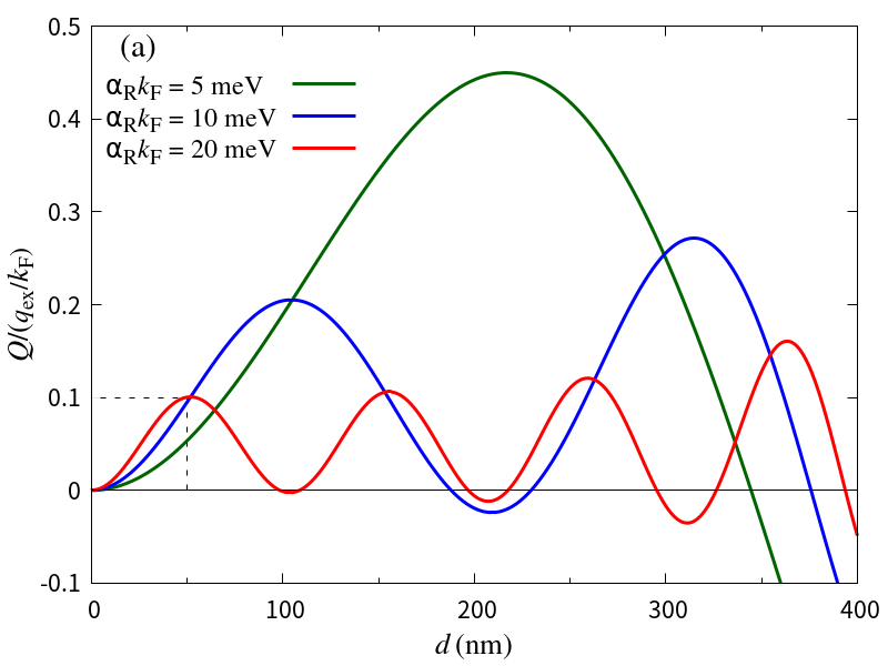
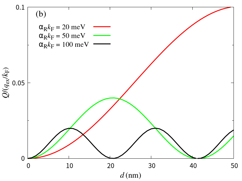
Figure 4: The $d$-dependence of $Q$ in units of $q_{ex}/k_{F}$ with $h_{y}$ = 10 T and $h_{z}$ = 0 T is plotted for (a) $\alpha_{R}k_{F}$=5 meV (green), 10 meV (blue), and 20 meV (red); (b) $\alpha_{R}k_{F}$=20 meV (red), 50 meV (light green), and 100 meV (black). The rectangular area in (a) denoted by the broken line corresponds to the plot area of (b). The red lines in (a) and (b) are the same line except for the plot area.

The rectangular area in (a) denoted by the broken line corresponds to the plot area of (b). The red lines in (a) and (b) are identical except for the plot area. The magnitude of $Q$ oscillates with $d$ and changes its sign. It means that the Josephson diode effect can be optimized by tuning of $d$. This provides a guiding principle for the Josephson diode device, because $d$ can be controlled in experiments. It is also important that the Josephson diode effect changes its sign with $d$, even when $\alpha_{R}$, $q_{ex}$ and $h_{y}$ are fixed. To determine not only the magnitude of the Josephson diode effect, but also its sign, we must take care of $d$ as well.

Increasing $\alpha_{R}k_{F}$, the period of the oscillation becomes short and the magnitude is suppressed. This can be understood by Eq. (55),

$$\delta{\cal V}_{o} \sim\frac{1}{2}\frac{q_{ex}}{k_{F}}\frac{\gamma h_{y}}{\alpha_{R}k_{F}}\left[\cos\left(\frac{2\gamma h_{y}d}{\hbar v_{F}}\right)-\cos\left(\frac{2\alpha_{R}k_{F}d}{\hbar v_{F}}\right)\right].$$ (59)

for $\alpha_{R}k_{F}\gg h_{y}$ and $h_{z}=0$. In Fig. 4, since $\gamma h_{y}=$ 1 meV is used, the second term of Eq. (59) dominates the $d$-dependence of $Q$ and the first term is almost 1 in the area of Fig. 4. Equation (59) is a decreasing function with respect to $\alpha_{R}k_{F}$. Therefore, the Josephson diode effect becomes smaller for larger values of $\alpha_{R}k_{F}$ as shown in Fig. 5.

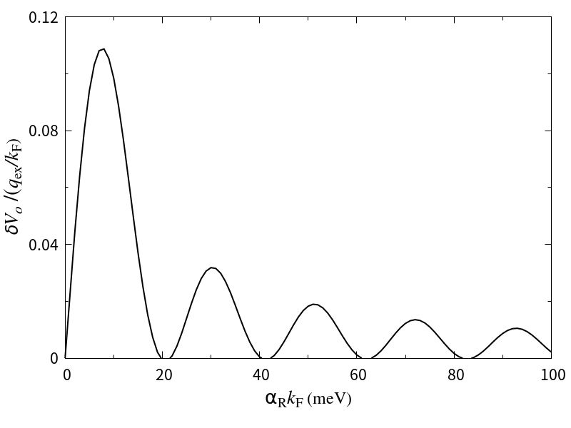
Figure 5: The $\alpha_{R}k_{F}$-dependence of $\delta{\cal V}_{o}$ with $d$ = 100 nm, and $h_{y}$ = 10 T, $h_{z}$ = 0 T.

Although the spin-orbit interaction is necessary for the Josephson diode effect, larger $\alpha_{R}$ does not always results in a larger effect. Sometimes the effect may accidentally disappear, e.g., $\alpha_{R}k_{F}\sim$ 20 meV in Fig. 5. In general, it is not easy to tune $\alpha_{R}k_{F}$, whereas $d$ can be controlled in experiment. Our results suggests that the Josephson diode effect can be optimized by tuning of $d$.

V Summary

We theoretically studied the Josephson diode effect in the Josephson junction with singlet superconductors separated by the Rashba system. The coupling energy of two superconductors was formulated under the bias current using a tunneling Hamiltonian with a one-dimensional model. The Josephson diode effect occurs as the response to the bias current. Therefore, including the bias current into the formulation is important to study the Josephson diode effect. The bias current is included in our formulation as the shifts of the Fermi momentum in the Rashba system. Due to the shift of Fermi momentum, the critical current is asymmetrically changed with respect to the current and the magnetic field. By including the bias current in the formulation, the first harmonic of the Josephson coupling can reproduces the Josephson diode effect. More importantly, the Josephson diode effect depends on the distance between superconducting electrodes $d$. In general, it is difficult to tune the band splitting by the spin-orbit interaction, whereas $d$ is experimentally controllable. Our findings suggest that the Josephson diode effect can be optimized by tuning of $d$. It will help to observe the Josephson diode effect experimentally. The magnitude of the Josephson diode effect is inversely proportional to the band split at the Fermi surface caused by the spin-orbit interaction. Although the spin-orbit interaction is necessary, larger $\alpha_{R}$ does not always results in a larger effect. Our theory develops a new guiding principle to design the Josephson diode device.

Appendix A Current-phase relation

The Josephson coupling energy under a current bias has not been formulated by the tunneling Hamiltonian. It is noted that $q_{ex}$ in Eq. (54) is a function of $i_{B}$ as discussed in Sec. IV, i.e., $q_{ex}=-2\pi i_{B}/|e|v_{d}$. Taking the derivative with respect to $\phi$ over the sum of Eq. (54) and the external force $i_{B}\cdot\phi$, we obtain the equation,

$$i_{B}=t^{4}{\cal U}{\cal V}_{bias}\sin\left(\phi-\frac{2\pi d}{|e|v_{d}}i_{B}\right).$$ (60)

Solving Eq. (60) with respect to $i_{B}$, the current-phase relation under the current bias is obtained as shown in Fig. 6,

Figure 6: The current-phase relation obtained by solving $y=\sin(x-a\!\cdot\!y)$ which is reduced from Eq. (60) with $y\equiv i_{B}$, $x\equiv\phi$, $a\equiv 2\pi d/|e|v_{d}$, and $t^{4}{\cal U}{\cal V}_{bias}=1$.

in which Eq. (60) is parameterized by $x\equiv\phi$, $y\equiv i_{B}$, and $a\equiv 2\pi d/|e|v_{d}$ and is reduced to $y=\sin\left(x-a\!\cdot\!y\right)$ with $t^{4}{\cal U}{\cal V}_{bias}=1$. The current-phase relation is modified as that of metallic interface by increasing $a$. When the parameter $a$ is much larger than 1, the current-phase relation deviates from the sinusoidal behavior. Since we adopted the one-dimensional model for the two-dimensional system, we cannot exactly assign the value of $a$. For studying the Josephson diode effect, we assumed that the current phase relation is a periodic function like that in Fig. 6. Although the exact formulation of the current-phase relation under the current bias is not the main purpose of this study, it is also interesting and will be numerically studied using the two-dimensional system elsewhere in future.

References

- (1) A. M. Kadin, R. Burkhardt, J. D. Chen, J. E. Keem, and S. R. Ovshinsky, Proceedings of the 17th 1international Conference on Low Temperature Physics, LT 17, Karlsruhe (North-Holland, Amsterdam, 1984), p. 579.
- (2) P. R. Broussard and T. H. Geballe, Phys. Rev. B 37, 68 (1988).
- (3) N. Touitou, P. Bernstein, J.F. Hamet, Ch. Simon, L. Méchin, J.P. Contour, and E. Jacquet, Appl. Phys. Lett. 85, 1742 (2004).
- (4) F. Ando, Y. Miyasaka, T. Li, J. Ishizuka, T. Arakawa, Y. Shiota, T. Moriyama, Y. Yanase, and T. Ono, Nature 584, 7821 (2020).
- (5) Y. Miyasaka, R. Kawarazaki, H. Narita, F. Ando, Y. Ikeda, R. Hisatomi, A. Daido, Y. Shiota, T. Moriyama, Y. Yanase, and T. Ono Appl. Phys. Express 14, 073003 (2021).
- (6) R. Kawarazaki, H. Narita, Y. Miyasaka, Y. Ikeda, R. Hisatomi, A. Daido, Y. Shiota, T. Moriyama, Y. Yanase, A.V. Ognev, A.S. Samardak, and T. Ono, Appl. Phys. Express 15, 113001 (2022).
- (7) H. Narita, J. Ishizuka, R. Kawarazaki, D. Kan, Y. Shiota, T. Moriyama, Y. Shimakawa, A.V. Ognev, A.S. Samardak, Y. Yanase, and T. Ono, Nature Nanotech. 17, 823–828 (2022).
- (8) Y. Hou, F. Nichele, H. Chi, A. Lodesani, Y. Wu, M.F. Ritter, D.Z. Haxell, M. Davydova, S. Ilić, O. Glezakou-Elbert, A. Varambally, F.S. Bergeret, A. Kamra, L. Fu, P.A. Lee, and J.S. Moodera, Phys. Rev. Lett. 131, 027001 (2023).
- (9) V. M. Edelstein, J. Phys. Cond. Matt. 8, 339 (1996).
- (10) A. Daido, Y. Ikeda, and Y. Yanase, Phys. Rev. Lett. 128, 037001 (2022).
- (11) J. J. He, Y. Tanaka, and N. Nagaosa, New J. Phys. 24, 053014 (2022).
- (12) N. F. Q. Yuan and L. Fu, PNAS 119, e2119548119 (2022).
- (13) K. Aoyama, Phys. Rev. B 109, 024516 (2024).
- (14) C. Baumgartner, L. Fuchs, A. Costa, S. Reinhardt, S. Gronin, G. C. Gardner, T. Lindemann, M. J. Manfra, P. E. F. Junior, D. Kochan, J. Fabian, N. Paradiso, and C. Strunk, Nat. Nanotech. 17, 1 (2022).
- (15) K.-R. Jeon, J.-K. Kim, J. Yoon, J.-C. Jeon, H. Han, A. Cottet, T. Kontos, and S. S. P. Parkin, Nature Mater. 21, 1008 (2022).
- (16) B. Pal, A. Chakraborty, P.K. Sivakumar, M. Davydova, A.K. Gopi, A. K. Pandeya, J.A. Krieger, Y. Zhang, M. Date, S. Ju, N. Yuan, N. B. M. Schröter, L. Fu, and S. S. P. Parkin, Nat. Phys. 18, 1228 (2022).
- (17) H. Wu, Y. Wang, Y. Xu, P.K. Sivakumar, C. Pasco, U. Filippozzi, S. S. P. Parkin, Y.-J. Zeng, T. McQueen, and M. N. Ali, Nature 604, 653 (2022).
- (18) J.-K. Kim, K.-R. Jeon, P. K. Sivakumar, J. Jeon, C. Koerner, G. Woltersdorf, and S. S. P. Parkin, Nature Commun. 15, 1120 (2024).
- (19) E. Nikodem, J. Schluck, M. Geier, M. Papaj, H. F. Legg, J. Feng, M. Bagchi, L. Fu, and Y. Ando, arXiv:2412.16569.
- (20) E. I. Rashba, Sov. Phys. Solid State 2 1109 (1960).
- (21) Yu. A. Bychkov and E. I. Rashba, JETP Lett. 39, 78 (1984).
- (22) E. V. Bezuglyi, A. S. Rozhavsky, I. D. Vagner, and P. Wyder, Phys. Rev. B 66, 052508 (2002).
- (23) L. N. Bulaevskii, V.V. Kuzii, and A. A. Sobyanin, JETP Lett. 25, 290 (1977).
- (24) A. I. Buzdin, L. N. Bulaevskii, and S. V. Panyukov, JETP Lett. 35, 178 (1982).
- (25) V.V. Ryazanov, V.A. Oboznov, A.Yu. Rusanov, A.V. Veretennikov, A.A. Golubov, and J. Aarts, Phys. Rev. Lett. 86, 2427 (2001).
- (26) T. Kontos, M. Aprili, J. Lesueur, F. Genêt, B. Stephanidis, and R. Boursier, Phys. Rev. Lett. 89, 137007 (2002).
- (27) H. Sellier, C. Baraduc, F. Lefloch, and R. Calemczuk, Phys. Rev. B 68, 054531 (2003).
- (28) S. M. Frolov, D. J. Van Harlingen, V. A. Oboznov, V. V. Bolginov, and V. V. Ryazanov, Phys. Rev. B 70, 144505 (2004).
- (29) C. Bell, R. Loloee, G. Burnell, and M. G. Blamire, Phys. Rev. B 71, 180501R (2005).
- (30) V. A. Oboznov, V. V. Bolginov, A. K. Feofanov, V. V. Ryazanov, and A. I. Buzdin, Phys. Rev. Lett. 96, 197003 (2006).
- (31) V. Shelukhin, A. Tsukernik, M. Karpovski, Y. Blum, K. B. Efetov, A. F. Volkov, T. Champel, M. Eschrig, T. Loefwander, G. Schoen, and A. Palevski, Phys. Rev. B 71, 174506 (2006)
- (32) J. W. A. Robinson, S. Piano, G. Burnell, C. Bell, and M. G. Blamire, Phys. Rev. Lett. 97, 177003 (2006).
- (33) F. Born, M. Siegel, E. K. Hollmann, H. Braak, A. A. Golubov, D. Yu. Gusakova and M. Yu. Kupriyanov: Phys. Rev. B 74, 140501 (2006).
- (34) M. Weides, M. Kemmler, H. Kohlstedt, R. Waser, D. Koelle, R. Kleiner, and E. Goldobin: Phys. Rev. Lett. 97, 247001 (2006).
- (35) T. Yamashita, K. Tanikawa, S. Takahashi, and S. Maekawa, Phys. Rev. Lett. 95 (2005) 097001
- (36) T. Yamashita, S. Kim, H. Kato, W. Qiu, K. Semba, A. Fujimaki, and H. Terai, Sci. Rep. 10, 13687 (2020).
- (37) A. Buzdin, Phys. Rev. Lett. 101, 107005 (2008).
- (38) T. Yokoyama, M. Eto, and Y. V. Nazarov, Phys. Rev. B 89, 195407 (2014).
- (39) Y. Zhang, Y. Gu, P. Li, J. Hu, and K. Jiang, Phys. Rev. X 12, 041013 (2022).
- (40) M. Davydova, S. Prembabu, and L. Fu, Science Adv. 8, eabo0309 (2022).
- (41) R. S. Souto, M. Leijnse, and C. Schrade, Phys. Rev. Lett. 129, 267702 (2022).
- (42) Y. Tanaka, B. Lu, and N. Nagaosa, Phys. Rev. B 106, 214524 (2022).
- (43) B. Lu, S. Ikegaya, P. Burset, Y. Tanaka, and N. Nagaosa, Phys. Rev. Lett. 131, 096001 (2023).
- (44) J.-X. Hu, Z.-T. Sun, Y.-M. Xie, and K. T. Law, Phys. Rev. Lett. 130, 266003 (2023).
- (45) P.-H. Fu, Y. Xu, S. A. Yang, C. H. Lee, Y. S. Ang, and J.-F. Liu, Phys. Rev. Appl. 21, 054057 (2024).
- (46) J. Cayao, N. Nagaosa, and Y. Tanaka, Phys. Rev. B 109, L081405 (2024).
- (47) D. Debnath and P. Dutta, Phys. Rev. B 109, 174511 (2024).
- (48) A. Soori, J. Phys. Cond. Mat. 36, 335303 (2024).
- (49) S. Fracassi, S. Traverso, N. Traverso Ziani, M. Carrega, S. Heun, and M. Sassetti, Appl. Phys. Lett. 124, 242601 (2024).
- (50) Y. Yerin, S.-L. Drechsler, A. A. Varlamov, M. Cuoco, and F. Giazotto, Phys. Rev. B 110, (2024).
- (51) S. Ilić, P. Virtanen, D. Crawford, T. T. Heikkilä, and F. S. Bergeret, Phys. Rev, B 110, L140501 (2024).
- (52) A. Soori, J. Phys. Cond. Mat. 37, 10LT02 (2025).
- (53) D. Debnath and P. Dutta, arXiv:2411.18325.
- (54) In the vector representation, it should be . In this paper, and are scaler.
- (55) M. Mori, S. Hikino, S. Takahashi, and S. Maekawa, J. Phys. Soc. Jpn. 76, 054705 (2007).
- (56) F. S. Bergeret, A. F. Volkov, and K. B. Efetov, Phys. Rev. B 64, 134506 (2001).
- (57) V. N. Krivoruchko and R. V. Petryuk, Phys. Rev. B 66, 134520 (2002).
- (58) S. Mironov, A. Mel’nikov, and A. Buzdin, Phys. Rev. Lett. 109, 237002 (2012).
- (59) A. S. Mel’nikov, S. V. Mironov, A. V. Samokhvalov, and A. I. Buzdin, Phys. Uspekhi 65, 1248 (2022).
- (60) The electronic current must be continuous through the junction. The total amount of current flowing in the superconductor has to be equal to that in the Rashba system. In order to understand the relation between and the supercurrent, it is useful to consider the conventional Josephson junction, i.e., the superconductor/insulator/superconductor (SIS) junction. The supercurrent in the SIS junction is related to the phase difference, which is equivalent to the magnetic flux, since the supercurrent is the diamagnetic current. This can be interpreted as: There is a vector potential between the left and right superconductors. In the junction via the Rashba system, on the other hand, the current flows in the Rashba system under the same condition as the SIS junction. It means that the vector potential is added to the Rashba system due to the phase difference between two superconductors. If a supercurrent flows in a junction with a phase difference, the same amount of current flows in the Rashba system due to the continuity of the current. Since the current is related to the vector potential, the momentum of electrons is shifted by the vector potential. Therefore, the shift of the Fermi momentum is necessary to satisfy the continuity of the electronic current through the junction.
- (61) We consider a current with 1 [A] flowing in a wire with 1 [mm] radius. For copper, using [cm-3] ashcroftmermin , it is estimated that [m/s]. For another case with small electron density such as GaAs with [cm-3], [m/s]. In fact, is much smaller than . On the other hand, will depend on materials and geometry, e.g., interface and surface.
- (62) N. W. Ashcroft and N. D. Mermin, Solid State Physics (Thomson Learning, USA, 1976) Chap. 2, p. 38.
- (63) The phase factor as a function of in Eq. (12) leads to and . To summarize the long calculation briefly, it is found that the center of mass momentum of Cooperon in the Rashba system is given by, and , where and corresponds to the momentum in and , respectively. Both of and shift the center of mass momentum of Cooperon. However, shifts the momentum out-of-phase, while does it in-phase. Due to this difference, leads to explaining the -junction, while shifts the phase difference as .
- (64) S. LaShell, B. A. McDougall, and E. Jensen, Phys. Rev. Lett. 77, 3419 (1996).
- (65) C. R. Ast, J. Henk, A. Ernst, L. Moreschini, M. C. Falub, D. Pacilé, P. Bruno, K. Kern, and M. Grioni, Phys. Rev. Lett. 98, 186807 (2007).
- (66) K. Ishizaka, M.S. Bahramy, H. Murakawa, M. Sakano, T. Shimojima, T. Sonobe, K. Koizumi, S. Shin, H. Miyahara, A. Kimura, K. Miyamoto, T. Okuda, H. Namatame, M. Taniguchi, R. Arita, N. Nagaosa, K. Kobayashi, Y. Murakami, R. Kumai, Y. Kaneko, Y. Onose, and Y. Tokura, Nature Mater. 10, 521 (2011).