Efficient Qubit Calibration by Binary-Search Hamiltonian Tracking

Abstract

We present a real-time method for calibrating the frequency of a resonantly driven qubit. The real-time processing capabilities of a classical controller dynamically generate adaptive probing sequences for qubit-frequency estimation. Each probing evolution time and drive frequency are calculated to divide the prior probability distribution into two branches, following a locally optimal strategy that mimics a conventional binary search. We show the algorithm’s efficacy by stabilizing a flux-tunable transmon qubit, leading to improved coherence and gate fidelity. By feeding forward the updated qubit frequency, the FPGA-powered control electronics partially mitigates non-Markovian noise in the system, which is detrimental to quantum error correction. Our protocol highlights the importance of feedback in improving the calibration and stability of qubits subject to drift and can be readily applied to other qubit platforms.

I Introduction

Quantum processing units (QPUs) with tens of qubits are becoming increasingly common [1]. Efforts to reduce error rates have resulted in the first demonstrations of quantum error correction [2, 3], though these advances come with costly calibration overhead as the number of qubits increases. Temporal instability in QPUs arises from numerous stochastic noise channels [4], and the lowest-performing outlier qubits often limit overall performance [5]. Tackling time-dependent fluctuations and outlier qubits in large QPUs requires scalable and efficient calibration methods to ensure stable, fault-tolerant operation while minimizing calibration downtime. We introduce here a protocol that features exponential scaling of the calibration precision versus the number of measurements until it is limited by decoherence. This scaling is the result of a locally optimal strategy that maximizes the expected precision for the next measurement.

Online Hamiltonian learning [6] offers a promising strategy for addressing drifts in stochastic qubit parameters through real-time estimation [6, 7, 8, 9, 10, 11, 12, 13], facilitated by modern field-programmable gate array (FPGA) hardware advancements. Although various estimation methods [14, 15, 16] have been proposed to enhance calibration efficiency, no experimental implementation has yet achieved real-time adaptive estimation in a resonantly driven qubit. This work fills the gap by the experimental demonstration of a real-time Bayesian estimation approach applied to a superconducting qubit.

To demonstrate the adaptive and efficient calibration protocol, we employ a flux-tunable transmon qubit [17, 18]. Transmons are largely insensitive to charge noise by design. The tunable qubit frequency is controlled by a magnetic field and it is susceptible to random flux variations, known as flux noise. Typically, flux-tunable transmons are thus operated at bias points (sweet spots) that are first-order insensitive to small flux changes. However, operating them away from these bias points may be necessary to reduce frequency crowding in large qubit arrays [19, 20] or minimize coupling to two-level fluctuators. To maintain high-fidelity operation despite the increased sensitivity to flux noise, one may use real-time frequency estimation and stabilization [21].

The so-called frequentist approach is the most common method for estimating fluctuations in Hamiltonian parameters of superconducting qubits. Frequentist estimation methods infer an observable from the observed frequencies of measurement outcomes in repeated experiments. For instance, in Ref. [21] the qubit frequency fluctuation is computed in real time by repeated Ramsey interferometry cycles. In the probing Ramsey cycle, the Bloch vector is initialized on the equator of the Bloch sphere, evolves under its Hamiltonian, and is projected back onto the $\hat{z}$-axis after a fixed (non-adaptive) evolution time. The measurement outcome is averaged over many probing cycles. The fraction of times the system is measured in the excited state, for instance, is linearly mapped to the qubit frequency fluctuation, as further detailed in the next section. The drawbacks of such frequentist methods are that (i) they are not optimally efficient, (ii) there is a trade-off between frequency sensitivity and probing range, and (iii) the qubit must already be approximately calibrated for the stabilization to work. In contrast, a Bayesian estimation approach assigns probabilities to hypotheses and naturally incorporates real-time optimization techniques [6, 8, 9, 10, 13]. At any given time, the current knowledge of the parameters can be used to adaptively select the optimal experimental settings for the next probing cycle.

In this work, we employ an adaptive Bayesian estimation scheme to calibrate a transmon qubit, which circumvents the limitations of the frequentist approach mentioned above. Our protocol involves programming a commercial controller with an integrated FPGA to generate dynamic microwave pulses, enabling real-time qubit frequency calibration through a binary search algorithm inspired by Ref. [22]. We use the real-time capabilities of the controller (on the qubit coherence timescale) to select optimal parameters within an adaptive estimation cycle. Specifically, the controller dynamically adjusts the drive frequency and the evolution time of each probing cycle based on previous measurement results. We demonstrate the algorithm’s efficacy through improved qubit coherence and fidelity.

While the majority of theoretical research concentrates on Markovian noise , non-Markovian noise sources such as $1/f$ flux noise, which exhibit memory effects, are common in solid-state qubit platforms [10]. They introduce significant overhead for error mitigation [24, 25], their dynamical decoupling [26, 27] is not universally effective and may not align with specific experimental goals. In order to realize fault-tolerant quantum computing with error-corrected solid-state qubits, non-Markovian noise likely needs to be reduced or eliminated  [28]. We show how our real-time frequency tracking protocol reduces such noise. Our scheme enables intermittent and efficient calibration of qubit frequencies, making it ideal for stable quantum circuit execution in the presence of drift.

II Method

II.1 Device

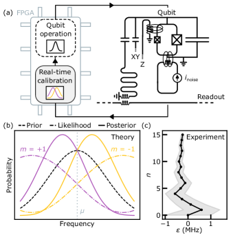
Figure 1: Qubit implementation and frequency binary search. (a) Experiment schedule, alternating between periods of quantum information processing (dashed box), and periods for efficiently calibrating the qubit frequency (gray box). The transmon (Qubit) is controlled by microwave pulses (XY) that are based on previous qubit measurements (Readout). (b) Evolution of the probability distribution ${\cal P}(\varepsilon)$ during the frequency binary search algorithm. For each Ramsey probing cycle, the probing time and frequency detuning are chosen such that the two possible likelihood functions (dash–dotted lines) multiplied with the prior distribution (dashed) yield posterior distributions (solid) that are shifted left or right, while the standard deviation is reduced (see main text). (c) The controller updates the probability distribution after each measurement. The dots show the resulting expectation value $\langle\varepsilon\rangle$ and the shaded area marks the 68% credible interval.

We use a $2\times 2$ superconducting qubit array operated at the mixing-chamber stage (below $30\text{\,}\mathrm{mK}$) of a dilution refrigerator. The array design is based on Ref. [29], and we calibrate one of its flux-tunable transmon qubits. A commercial controller (Quantum Machines OPX+ and Octave) applies high-frequency waveforms to the lines for qubit control and single-shot readout. A Yokogawa GS200 provides the DC flux bias through a bias-tee at room temperature (see the Supplemental Material [30] for details on the experimental setup). The transmon comprises a DC SQUID with asymmetric junctions, and on-chip Z and XY control lines [see Fig. 1(a)]. The qubit is dispersively coupled to a coplanar waveguide resonator for state readout [17, 18].

The real-time calibration we develop here can be embedded in an operation loop as sketched in Fig. 1(a). The calibration protocol is used to estimate the qubit frequency, after which the resulting estimate is used to adjust the frequency of the drive accordingly, leading to a decreased sensitivity to flux noise during qubit operation.

Our goal is to compensate for qubit frequency fluctuations particularly when it is operated away from the sweet spot. Thus we tune the transmon where the effect of flux noise is the strongest, at $\Phi_{\text{ext}}=\Phi_{0}/4$, where $\Phi_{0}=h/(2e)$ is the superconducting magnetic flux quantum and $\Phi_{\text{ext}}$ is the external magnetic flux applied via a mutual coupling to the Z line. Our qubit nominally has a transition frequency $f_{\text{q}}\approx$3.78\text{\,}\mathrm{GHz}$$ and in the rotating frame its Hamiltonian is

$$\frac{\mathcal{H}(t)}{h}=-\dfrac{\Updelta f-\varepsilon(t)}{2}\sigma_{z},$$ (1)

where $\sigma_{z}$ is the Pauli $z$-matrix, $\Updelta f=f_{\text{d}}-f_{\text{q}}$ is the frequency detuning between $f_{\text{q}}$ and the chosen rotating frame frequency $f_{\text{d}}$, and $\varepsilon(t)$ represents the time-dependent shift of the qubit frequency due to flux noise.

II.2 Frequency binary search by Bayesian estimation

The frequency binary search (FBS) algorithm involves a Ramsey probing cycle where the qubit is first prepared in a superposition state $\ket{\psi}=\left(\ket{0}-i\ket{1}\right)/\sqrt{2}$ using a X_π/2 rotation around the $\hat{x}$-axis of the Bloch sphere. The state preparation is followed by a period of free evolution for a duration $\tau$, during which the qubit state acquires a phase $\phi=2\pi\int_{0}^{\tau}\delta_{\text{q}}(t^{\prime})\,\mathrm{d}t^{\prime}$, where $\delta_{\text{q}}(t)=\Updelta f-\varepsilon(t)$. A second X_π/2 pulse is then applied, and the state of the qubit is measured using dispersive readout. By the quasistatic noise approximation, we assume $\varepsilon(t)$ to be constant on the scale of a few probing cycles, resulting in $\phi=2\pi[\Updelta f-\varepsilon(t)]\tau$. In the following, we drop the time dependence of $\varepsilon(t)$ for ease of notation.

We assume that the probability of measuring an outcome $m\in\{-1,1\}$ corresponding to the states $|0\rangle$ and $|1\rangle$ is given by the likelihood function

$$P(m|\varepsilon,\Updelta f,\tau)=\frac{1}{2}+\frac{m}{2}\{\alpha+\beta e^{-\tau/T}\cos{[2\pi(\Updelta f-\varepsilon)\tau]}\},$$ (2)

where the parameters $\alpha=-0.02$ and $\beta=0.6$ are coefficients that together capture state preparation and readout errors, while $T$ describes a coherence time that limits the duration of the evolution time $\tau$ (see the Supplemental Material [30] for further details on how they impact the algorithm performance). We set $T\approx$10\text{\,}\mathrm{\SIUnitSymbolMicro s}$$ based on the Hahn echo coherence time $T_{2\text{E}}\approx$12\text{\,}\mathrm{\SIUnitSymbolMicro s}$$. The qubit fluctuation $\varepsilon$ is what we want the controller to estimate.

We emphasize that in this experiment the controller adaptively computes in real time both the Ramsey evolution time $\tau$ and the drive frequency $f_{\text{d}}$ (and thus $\Updelta f$) for each probing cycle. This differs from previously employed approaches where (i) the evolution time $\tau$ is fixed [21] and (ii) only either the evolution time $\tau$ or the effective rotating frame frequency is chosen adaptively [31, 8, 13]. We also highlight that using a fixed evolution time $\tau$ in non-adaptive probing cycles [21] limits the frequency range to $\left(-\frac{1}{2\tau},+\frac{1}{2\tau}\right]$, which results in a trade-off between range and frequency sensitivity. This trade-off does not apply to the binary search algorithm introduced here.

In the quasistatic approximation, we want to find the optimal sequence of $\tau$’s and $f_{\text{d}}$’s to estimate $\varepsilon$ in as few measurements as possible. Using Bayes’ rule we write

$${\cal P}_{n+1}(\varepsilon)\propto{\cal P}_{n}(\varepsilon)P(m_{n+1}|\varepsilon,\Updelta f_{n+1},\tau_{n+1}),$$ (3)

where ${\cal P}_{n}(\varepsilon)$ denotes the probability distribution for $\varepsilon$ after the $n^{\text{th}}$ probing cycle, which thus depends on all previously used $\Updelta f_{i}$ and $\tau_{i}$ and all measurement outcomes $m_{i}$ (i.e., $i\leq n$).

In the following we assume ${\cal P}_{n}(\varepsilon)$ to be a Gaussian, which well approximates the actual distribution (see the Supplemental Material [30] for more details). The advantage of using the Gaussian approximation is that it allows the distribution to be conveniently described using just two parameters: the mean $\mu$ and the standard deviation $\sigma$.

For each individual probing cycle, to minimize the expected posterior variance, in a greedy approach the optimal experiment $(\tau,\Updelta f)$ is the one that divides the prior distribution into equal (or approximately equal) left and right portions [see Fig. 1(b)] so that a half period of Eq. (2) is comparable to the width of the prior distribution, performing something similar to a binary search partitioning . The approach of using Gaussians and partitioning the posterior distributions in a similar fashion was introduced by Ref. [22]. However, in that case, the lack of phase control in the likelihood prevents the algorithm from determining the sign of $\varepsilon$, making it ineffective for priors where $\mu/\sigma\rightarrow 0$ . While fitting to a bimodal Gaussian has been suggested as a solution [34], this approach still does not resolve the ambiguity of the sign. In this work, we address both aspects by dynamically updating $f_{\text{d}}$ (and thus $\Updelta f$) in real time on the controller. This allows the controller to consistently use the optimal likelihood function and perform the most efficient estimation using only a Gaussian distribution.

Two steps are needed to implement the binary search in the controller. The first step is to determine optimal experiment parameters $\tau$ and $\Updelta f$ based on the prior distribution. Then, one must approximate the resulting posterior ${\cal P}_{n+1}(\varepsilon)$ to a Gaussian. This can be done using equations implemented directly on the controller in real time.

The prior distribution, dashed black line in Fig. 1(b), in the Gaussian approximation is given by

$${\cal P}_{n}(\varepsilon)=\frac{1}{\sqrt{2\pi\sigma_{n}^{2}}}\exp{-\left(\frac{\varepsilon-\mu_{n}}{\sqrt{2}\sigma_{n}}\right)^{2}},$$ (4)

where $\mu_{n}$ is our guess for what $\varepsilon$ is with uncertainty $\sigma_{n}$. In order to separate the prior at the center by the likelihood functions, the detuned frequency must satisfy

$$\Updelta f_{n+1}=\frac{1+2l}{4\tau_{n+1}}+\mu_{n},$$ (5)

where $l$ can be any integer number; we set it to be zero. While this is formally the optimal solution for $\alpha=0$, it is a reasonable approximation for the optimum at other realistic values of $\alpha$. Given this constraint, the optimal evolution time $\tau$ that minimizes the posterior variance is given by:

$$\tau_{n+1}=\frac{\sqrt{16\pi^{2}\sigma_{n}^{2}+1/T^{2}}-1/T}{8\pi^{2}\sigma_{n}^{2}}.$$ (6)

After measuring $m_{n+1}=\pm 1$, the posterior distribution is obtained by using Eq. (3), after which it is fit to a Gaussian using the method of moments, i.e., by calculating its mean and variance [22]

$$\mu_{n+1} =\mu_{n}-\frac{2\pi m_{n+1}\beta\sigma_{n}^{2}\tau_{n+1}e^{-\tau_{n+1}/T-2\pi^{2}\sigma_{n}^{2}\tau_{n+1}^{2}}}{1+m_{n+1}\alpha},$$ (7a)

$$\sigma_{n+1}^{2} =\sigma_{n}^{2}-\frac{4\pi^{2}\beta^{2}\sigma_{n}^{4}\tau_{n+1}^{2}e^{-2\tau_{n+1}/T-4\pi^{2}\sigma_{n}^{2}\tau_{n+1}^{2}}}{(1+m_{n+1}\alpha)^{2}},$$ (7b)

and using these values to construct the new prior to be a Gaussian distribution with mean and variance $\mu_{n+1}$ and $\sigma^{2}_{n+1}$ [see Fig. 1(b)]. This scheme is repeated $N$ times to obtain a sufficiently narrow distribution with exponential scaling given by Eq. (7b).

In Fig. 1(c) we illustrate the resulting evolution of ${\cal P}_{n}(\varepsilon)$ as a function of the measurement number $n$ for one representative estimation sequence, with an initial prior with $\sigma_{0}=$1\text{\,}\mathrm{MHz}$$ and $\mu_{0}=0$, and $N=15$. The black dots show the expectation value $\langle\varepsilon\rangle$, and the shaded area indicates its 68% credible interval, narrowing here down to $67\text{\,}\mathrm{kHz}$ after 15 measurements.

In the following, we optimize the number of single-shot measurements $N$ we use based on the specific experiment we are performing. We test the performance of the FBS by performing Ramsey repetitions to verify that it finds the correct qubit frequency, and we use randomized benchmarking and gate set tomography to assess the impact of the FBS on the qubit fidelity and drift. We emphasize again that the goal of these experiments is not to increase qubit coherence or fidelity as much as possible, but simply to confirm that the information gained from the FBS is most likely correct.

III Results

III.1 Qubit coherence

Figure 2: Frequency binary search validation by suppressed dephasing of a qubit in a feedback-controlled rotating frame. (upper diagram) One loop (solid arrows) represents one repetition of the protocol. (a) For each estimate of the frequency shift $\varepsilon$, the controller uses $N=8$ Ramsey probing cycles with adaptive probe times $\tau_{i}$ and detuned frequencies $\Updelta f_{i}$, computed in real time. Bottom panel: $\langle\varepsilon\rangle$ (solid line) and 68% credible interval (shaded area) of the final probability distribution ${\cal P}_{8}(\varepsilon)$ of all estimates performed during the $\approx$24\text{\,}\mathrm{s}$$ of the experiment. (b) After each estimation, we task the controller to perform a Ramsey cycle with evolution time $\tau_{j}$, while setting $\Updelta f_{j}=$1\text{\,}\mathrm{MHz}$$ by adjusting $f_{\rm d}$ using the latest estimate $\langle\varepsilon\rangle$. These interleaved FBS estimations and Ramsey cycles are repeated $M=50$ times with evenly spaced $\tau_{j}$. Single-shot measurement outcomes $p_{j}$ are plotted in the middle panel as white/black pixels, and the fraction of flipped outcomes in each column is shown as a blue dot in the lower panel. (c) Subsequently the controller resets all frequencies to the offline-calibrated values, i.e., assumes $\langle\varepsilon\rangle=0$, and performs again $M=50$ evenly spaced Ramsey cycles of set $\Updelta f_{k}=$1\text{\,}\mathrm{MHz}$$. Single-shot measurement outcomes $q_{k}$ are plotted as white/black pixels in the middle panel, and the fraction of flipped outcomes in each column is shown as a red dot in the lower panel. Comparing (b) to (c), the coherence time improves by $\approx 49\%$ with feedback.

We thus validate the FBS by rapid estimation of the shift of the qubit frequency $\varepsilon$ and demonstrating an extended coherence of the flux-tunable transmon qubit.

The fluctuating parameter $\varepsilon$ is estimated from the probing sequence shown in the top part of Fig. 2(a): For each probe cycle, the Bloch vector is positioned on the equator using an X_π/2 pulse. After precessing for a time $\tau_{i}$, a virtual Z$(\Updelta f_{i})$ gate [35] is performed, introducing a phase offset $\phi=2\pi\Updelta f_{i}\tau_{i}$. Here, virtual means that the phase offset is added to the subsequent X_π/2 pulse, which projects the Bloch vector back onto the $\hat{z}$-axis. This is followed by a measurement, after which the qubit state $s_{i}$, ground ($s_{i}=0$) or excited ($s_{i}=1$), is assigned by thresholding the demodulated dispersive readout signal on the controller.

The Bayesian probability distribution of $\varepsilon$ is updated after comparing the measurement outcome $s_{i}$ to the previous one $s_{i-1}$, as we do not initialize the qubit to the ground state at the beginning of each cycle to reduce the probing cycle period (thus yielding higher feedback bandwidth). It follows that in Eq. (2) $m_{i}=2|s_{i}-s_{i-1}|-1$. For instance, if in the previous measurement the qubit was in the ground state $s_{i-1}=0$ and now it is in the excited state ($s_{i}=1$) then $m_{i}=+1$. The duration of the probe cycle is short compared to the measured $T_{1}\approx$80\text{\,}\mathrm{\SIUnitSymbolMicro s}$$ at quarter flux: the average Ramsey evolution time is $\approx$4.36\text{\,}\mathrm{\SIUnitSymbolMicro s}$$, the time used to read out the qubit is $1.44\text{\,}\mathrm{\SIUnitSymbolMicro s}$, and the time used to subsequently cool down the resonator again (to deplete it from any residual photons after the readout pulse) is $\approx$2\text{\,}\mathrm{\SIUnitSymbolMicro s}$$.

The controller is programmed to start from a prior with $\mu_{0}=0$ and $\sigma_{0}=$30\text{\,}\mathrm{kHz}$$ based on previously measured qubit frequency fluctuations. After each measurement, the controller updates the probability distribution, resulting in a narrowing of the width of the distribution [cf. Fig. 1(c)]. In the middle panel of Fig. 2(a) we plot the experimentally found final posterior probability distributions ${\cal P}_{N}(\varepsilon)$ from all estimations done in the full experiment, where we consistently use $N=8$ measurements per estimation sequence. For plotting clarity we down-sample to $\approx$8\text{\,}\mathrm{ms}$$.

To confirm that these narrowed distribution functions indeed represent more accurate and correct knowledge about $\varepsilon$, we interleave the estimations with a series of Ramsey repetitions, half of them making use of the outcome of the estimations and half of them not, as shown schematically in the upper part of Fig. 2. After each estimation sequence of $\varepsilon$, the controller updates the qubit-frequency parameter $f_{\text{q}}$ (in software) to compensate for the estimated shift $\langle\varepsilon\rangle$, so that the total expected detuning becomes $\Updelta f_{j}-\langle\varepsilon\rangle=$1\text{\,}\mathrm{MHz}$$. Then it performs one Ramsey cycle with evolution time $\tau_{j}$, after which it again estimates $\varepsilon$. This cycle is repeated $M=50$ times, while $\tau_{j}$ is increased linearly from 0 to $7\text{\,}\mathrm{\SIUnitSymbolMicro s}$. Each row in the middle panel of Fig. 2(b) shows the result of one such set of 50 Ramsey cycles, where we plot all single-shot measurement outcomes $p_{j}$ as white/black pixels. After each set of $M=50$ Ramsey cycles with feedback, the controller resets $f_{\text{q}}$ (in software) to the offline-calibrated value, tuning to $\Updelta f_{k}=$1\text{\,}\mathrm{MHz}$$. It then performs the same series of 50 Ramsey cycles as before, linearly stepping the evolution time $\tau_{k}$ from 0 to $7\text{\,}\mathrm{\SIUnitSymbolMicro s}$. The rows in the middle panel of Fig. 2(c) show the single-shot measurement outcomes of this part of the protocol. After completing the Ramsey cycles without feedback, the whole protocol is repeated, as indicated in the top of Fig. 2, starting with a new estimation of $\varepsilon$. In the new estimation sequence, the controller starts from a prior with $\mu_{0}$ equal to the estimated $\varepsilon$ of the previous sequence.

To highlight the effect of the feedback, we plot the averages of all Ramsey repetitions in the lower panels of Fig. 2(b,c). In both cases, we fit the decaying signal using Gaussian envelopes (solid line), yielding $T_{2}=$3.73(0.11)\text{\,}\mathrm{\SIUnitSymbolMicro s}$$ without feedback and $T_{2}=$5.57(0.09)\text{\,}\mathrm{\SIUnitSymbolMicro s}$$ with feedback, corresponding to a $\approx 49$% improvement when including feedback. This increased coherence of the qubit demonstrates that the narrowed distribution function obtained from the estimation procedure indeed reflects more accurate knowledge about the fluctuating parameter $\varepsilon$. Notably, our approach requires fewer single-shot measurement outcomes ($N=8$) compared to $N=20$ of Ref. [21]. We perform another experiment for 6 hours, showing that the FBS keeps track of the qubit frequency also over longer time scales (see the Supplemental Material [30]). Overall, the results presented in this section show how the FBS can efficiently find and stabilize the qubit frequency.

III.2 Single-qubit gate fidelity

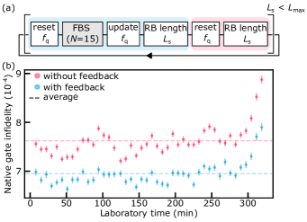
Figure 3: Frequency binary search validation by randomized benchmarking. (a) A randomized benchmarking repetition of length $L_{\text{s}}$ combined with the FBS feedback (with $N=15$ probing cycles). (b) Randomized benchmarking is repeated 44 times with the feedback (blue dots) and without (red dots). The native gate errors are extracted from the fit to the data, which consists of 10,000 realizations of 30 random Clifford sequences with and without the feedback. The error bars show the 68% confidence interval for the fitted gate error. Dashed lines are the averaged gate infidelities.

In this section we further validate the FBS calibration by showing improvement of the single-qubit gate fidelity by randomized benchmarking (RB) [36].

The pulse sequence is shown in Fig. 3(a): the controller resets the qubit-frequency parameter $f_{\text{q}}$ (in software), and it performs the FBS with $N=15$ probing sequences, starting with $\mu_{0}=0$ and $\sigma_{0}=$200\text{\,}\mathrm{kHz}$$ . At the end of the estimation, $f_{\text{q}}$ is updated (in software) and an RB sequence of depth $L_{\text{s}}$ is performed. An interleaved RB measurement without feedback follows by resetting the qubit frequency to the offline-calibrated value. The maximum circuit depth ($L_{\text{max}}$) is 2,300, and the repetition is averaged 10,000 times. We implement DRAG (derivative reduction by adiabatic gate) for our $20\text{\,}\mathrm{ns}$-long pulses to suppress leakage errors [17, 18] in the RB experiment. As with the previous experiment, the qubit is not initialized in the ground state at the beginning of each cycle; the controller keeps track of whether the state is different or not compared to the previous measurement. Every 1,000 averages, the threshold that classifies the demodulated dispersive readout signal is updated online in the controller by taking the average of 10,000 single-shot measurements after performing an X_π/2 pulse to the qubit.

The controller performs the RB experiment for 6 hours, yielding a native gate infidelity of $(7.6\pm 0.3)\times 10^{-4}$ without feedback and $(6.9\pm 0.2)\times 10^{-4}$ with feedback [dashed lines in Fig. 3(b)]. The single-qubit gate infidelities are higher than the decoherence limit [38] approximated by $t_{\text{gate}}(1/T_{1}+1/T_{\phi})/3\approx 6\times 10^{-4}$, given $t_{\text{gate}}\approx$20\text{\,}\mathrm{ns}$$, $T_{1}\approx$80\text{\,}\mathrm{\SIUnitSymbolMicro s}$$ and the exponential part of the pure dephasing time $T_{\phi}\approx$13\text{\,}\mathrm{\SIUnitSymbolMicro s}$$. The feedback protocol always performs better than without feedback, and with less spread around the mean value as a result of the stabilization. Some of the drifts of the infidelity remain correlated, which we tentatively attribute to other factors (e.g., changes in $T_{1}$). The improved fidelities of single-qubit gates by feedback by interleaved RB are presented in the Supplemental Material [30]. We attribute the smaller relative improvement in the single-qubit gate qubit fidelity, compared to coherence in the previous section, to the larger final value of $\sigma_{N=15}\approx$90\text{\,}\mathrm{kHz}$$, as opposed to $\sigma_{N=8}\approx$24\text{\,}\mathrm{kHz}$$, which resulted from different initial prior distributions.

III.3 Reduction of non-Markovian noise

So far, we have demonstrated an efficient qubit calibration protocol by instructing a controller to generate adaptive probing sequences in real time. The calibration has been validated by improved coherence and fidelity. Next, we investigate if our estimation protocol also reduces the non-Markovian noise in the system, this time estimated by gate set tomography [39].

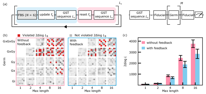
Figure 4: Gate set tomography and model violation. (a) A gate set tomography (GST) sequence combined with the FBS feedback (with $N=6$ probing cycles). (b) Model violation plot without (left) and with (right) FBS feedback. The red marks reveal detection of model violation at a confidence level of more than 95% and the gray boxes indicate statistical fluctuations. (c) The FBS feedback decreases the total amount of the log-likelihood ratios $2\Updelta\log L$ at maximum lengths of 4, 8, and 16, extracted from 30 GST runs. Error bars show the 68% credible interval.

Gate set tomography (GST) is a calibration-free method for benchmarking and characterizing operations in a quantum processor and we implement it by using the pyGSTi [40] software package. GST relies on running circuits designed to amplify certain types of errors. Each circuit, as shown in the right panel of Fig. 4(a), consists of the gate to be characterized, $\{G_{\text{I}},G_{\text{x}},G_{\text{y}},G_{\text{x}}G_{\text{y}},G_{\text{x}}G_{\text{x}}G_{\text{y}}\}$ (the germs), sandwiched between two fiducial circuits from the set $\{\text{I},\text{X}_{\pi/2},\text{Y}_{\pi/2},\text{X}_{\pi/2}\text{X}_{\pi/2},\text{X}_{\pi/2}\text{X}_{\pi/2}\text{X}_{\pi/2},\text{Y}_{\pi/2}\text{Y}_{\pi/2}\text{Y}_{\pi/2}\}$. These are applied to the qubit after initialization, to generate the state $\rho_{i}$, and before the measurement in the computational basis, to measure the operator $E_{j}$. The variable $L_{\text{s}}$ is the maximum depth used to construct the base circuit from the germ [39]. By running the circuit multiple times, we extract the measurement probabilities $P_{ji}=\Tr{E_{j}G[\rho_{i}]}$, which are then fitted to the error model, providing a maximum likelihood estimator of the transfer matrix for all of the gates. The quality of the fit can be used to detect violations of the Markovian model of the noise [39, 41].

We incorporate the feedback loop inside the GST protocol using the scheme shown in the left panel of Fig. 4(a), implemented on the controller. We find suitable parameters for testing the FBS to be $N=6$ per estimation sequence with feedback, with initial $\mu_{0}=0$ and $\sigma_{0}=$30\text{\,}\mathrm{kHz}$$. Each repetition is executed 100 times for each of the 616 sequences constructed for GST. In the new estimation sequence, the controller starts from a prior with $\mu_{0}$ equal to the estimated $\varepsilon$ of the previous repetition.

The measured discrepancy between the Markovian model and the data ($2\Updelta\log L_{\text{s}}$ as defined in Ref. [39]) is shown in Fig. 4(b) using the color of the squares: The grayscale is used to reflect the total discrepancy and a red color signals a model violation, indicating non-Markovian noise at 95% confidence interval. The rows and columns of the inner matrices represent the fiducial operations used for state preparation and measurement respectively. For the data with feedback, represented in the right panel of Fig. 4(b), a clear decrease in the number of red squares in comparison to the feedback-free result of the left panel is visible.

To further quantify the reduction of non-Markovian noise, the controller repeats the GST experiment 30 times, spanning a laboratory time of 40 minutes. In Fig. 4(c), we plot, as a function of the maximum length, the total violation of the model. While there is no clear improvement for maximum lengths of 1 and 2, it is evident for longer sequences. This is consistent with the expectation that longer circuits are more sensitive to non-Markovian noise [39].

Regarding gate performance, the GST protocol yields an X_π/2-pulse infidelity of $(2.6\pm 0.3)\times 10^{-2}$ and for the Y_π/2-pulse $(1.6\pm 0.3)\times 10^{-2}$, both with and without feedback. These values are two orders of magnitude larger than those reported by RB, which further suggests the dominant role of coherent noise, to which RB is less sensitive [42].

In summary, the decrease in Markovian model violation for longer GST sequences indicates that the FBS feedback protocol mitigates a significant portion of non-Markovian noise.

IV Outlook

Our work presents the experimental demonstration of a greedy adaptive Bayesian estimation protocol for the frequency of a resonantly driven qubit, extending its coherence using only $N=8$ single-shot measurements. Our approach reduces qubit-frequency drift by real-time Bayesian estimation and feedback, implemented via a low-latency FPGA-based qubit control system.

The binary search estimation algorithm allows control pulses to compensate for qubit frequency fluctuations caused by flux noise, improving coherence and fidelity without sacrificing frequency sensitivity or range. We validate the protocol using gate set tomography, which further corroborates our claim that our adaptive feedback loop reduces the effects of non-Markovian noise. This may facilitate quantum error correction methods, which generally assume Markovian noise.

Our protocol assumes that a Gaussian distribution can approximate the frequency fluctuations and that these remain constant over the time scale of a few measurements. In this work, the controller updates the drive frequency in real time, but the scheme can be adapted to adjust the qubit frequency by modifying the flux bias instead. The estimation bandwidth is limited by the relatively slow measurement time of a few microseconds. From this perspective, our work represents a worst-case scenario, underlying the efficacy of our experimental technique.

We anticipate further improvements possibly by the implementation of a physics-informed prior [13] that accounts for $1/f$ noise. Also, the online calibration of single-qubit gates is a possible direction with available hardware, for single-qubit corrections in two-qubit gates by actual (not virtual) Z gates. Adaptive Bayesian techniques could be implemented for frequency tracking in the presence of two-level fluctuators [43, 44]. Specific to our flux-tunable transmon qubit, while the feedback bandwidth is limited by readout and resonator cooldown time, higher bandwidth can be achieved by adding a Purcell filter [17, 18] which protects the qubit from relaxing into its environment. The use of feedback approaches may favor using symmetric junctions to increase the frequency range of the qubit, without worrying about increased sensitivity to flux noise.

Although qubit calibration by Bayesian inference can be relatively easily integrated with existing classical control hardware, it requires prior knowledge of the system’s parametrization. We expect that quantum model learning agents [6], which are more challenging to implement efficiently in real time, will gain wider adoption. We anticipate further research that merges theoretical and hardware advances, ultimately eliminating the need for a case-to-case modeling of experimental parameters.

Beyond superconducting qubits, our scheme offers new insights into real-time calibration of any qubits manipulated by resonant pulses. This work advances quantum control by implementing an adaptive Bayesian technique to calibrate the qubits frequencies in real time. Our algorithm is a locally optimal solution by minimizing the expected estimator variance under a Gaussian distribution approximation, making it appealing for real-time calibration in large QPUs.

V Author contributions

FB, JB, and JAK conceptualized the experiment. FB led the measurements and data analysis, and wrote the manuscript with input from all authors. FB, LP, MM, RA, AC, JAG, WDO, and FK performed the experiment with theoretical contributions from JB, JAK, and JD. YS designed the device, which was fabricated by DKK and BMN under supervision of KS, MES, and JLY. JAG, JD, WDO, and FK supervised the project.

VI Acknowledgments

We gratefully acknowledge Patrick Harrington and Max Hays for fruitful discussions. This work received funding from the European Union’s Horizon 2020 research and innovation programme under grant agreements 101017733 (QuantERA II), 951852 (QLSI), EUREKA Eurostars 3 (ECHIDNA), European Research Council (ERC grant 856526), the Novo Nordisk Foundation under Challenge Programme NNF20OC0060019 (SolidQ), the Inge Lehmann Programme of the Independent Research Fund Denmark, the US Army Research Office (ARO) under Award No. W911NF-24-2-0043, the QuSpin Mobility Grant, the INTFELLES-Project No. 333990, which is funded by the Research Council of Norway (RCN), the Dutch National Growth Fund (NGF) as part of the Quantum Delta NL programme, and from the Danish Agency for Higher Education and Science (DAHES, grant 2076-00014B). It was also funded in part by the US Army Research Office (ARO) Multidisciplinary University Research Initiative (MURI) W911NF-18-1-0218, in part by the US Army Research Office (ARO) under Award No. W911NF-23-1-0045, and in part under Air Force Contract No. FA8702-15-D-0001. Any opinions, findings, conclusions or recommendations expressed in this material are those of the author(s) and do not necessarily reflect the views of the US Air Force or the US Government.

*

References

- Ichikawa et al. [2024] T. Ichikawa, H. Hakoshima, K. Inui, K. Ito, R. Matsuda, K. Mitarai, K. Miyamoto, W. Mizukami, K. Mizuta, T. Mori, Y. Nakano, A. Nakayama, K. N. Okada, T. Sugimoto, S. Takahira, N. Takemori, S. Tsukano, H. Ueda, R. Watanabe, Y. Yoshida, and K. Fujii, Current numbers of qubits and their uses, Nature Reviews Physics 6, 345 (2024).
- Campbell [2024] E. Campbell, A series of fast-paced advances in quantum error correction, Nature Reviews Physics 6, 160 (2024).
- Acharya et al. [2024] R. Acharya, L. Aghababaie-Beni, I. Aleiner, T. I. Andersen, M. Ansmann, F. Arute, K. Arya, A. Asfaw, N. Astrakhantsev, J. Atalaya, et al., Quantum error correction below the surface code threshold 10.48550/arXiv.2408.13687 (2024).
- Ball et al. [2016] H. Ball, W. D. Oliver, and M. J. Biercuk, The role of master clock stability in quantum information processing, npj Quantum Information 2, 1 (2016).
- Mohseni et al. [2024] M. Mohseni, A. Scherer, K. G. Johnson, O. Wertheim, M. Otten, N. A. Aadit, K. M. Bresniker, K. Y. Camsari, B. Chapman, S. Chatterjee, G. A. Dagnew, A. Esposito, F. Fahim, M. Fiorentino, A. Khalid, X. Kong, B. Kulchytskyy, R. Li, P. A. Lott, I. L. Markov, R. F. McDermott, G. Pedretti, A. Gajjar, A. Silva, J. Sorebo, P. Spentzouris, Z. Steiner, B. Torosov, D. Venturelli, R. J. Visser, Z. Webb, X. Zhan, Y. Cohen, P. Ronagh, A. Ho, R. G. Beausoleil, and J. M. Martinis, How to build a quantum supercomputer: Scaling challenges and opportunities 10.48550/arXiv.2411.10406 (2024).
- Gebhart et al. [2023] V. Gebhart, R. Santagati, A. A. Gentile, E. M. Gauger, D. Craig, N. Ares, L. Banchi, F. Marquardt, L. Pezzè, and C. Bonato, Learning quantum systems, Nature Reviews Physics 5, 141 (2023).
- Reuer et al. [2023] K. Reuer, J. Landgraf, T. Fösel, J. O’Sullivan, L. Beltrán, A. Akin, G. J. Norris, A. Remm, M. Kerschbaum, J.-C. Besse, et al., Realizing a deep reinforcement learning agent for real-time quantum feedback, Nature Communications 14, 7138 (2023).
- Arshad et al. [2024] M. J. Arshad, C. Bekker, B. Haylock, K. Skrzypczak, D. White, B. Griffiths, J. Gore, G. W. Morley, P. Salter, J. Smith, I. Zohar, A. Finkler, Y. Altmann, E. M. Gauger, and C. Bonato, Real-time adaptive estimation of decoherence timescales for a single qubit, Physical Review Applied 21, 024026 (2024).
- Berritta et al. [2024a] F. Berritta, T. Rasmussen, J. A. Krzywda, J. van der Heijden, F. Fedele, S. Fallahi, G. C. Gardner, M. J. Manfra, E. van Nieuwenburg, J. Danon, A. Chatterjee, and F. Kuemmeth, Real-time two-axis control of a spin qubit, Nature Communications 15, 1676 (2024a).
- Park et al. [2024] J. Park, H. Jang, H. Sohn, J. Yun, Y. Song, B. Kang, L. E. A. Stehouwer, D. D. Esposti, G. Scappucci, and D. Kim, Passive and active suppression of transduced noise in silicon spin qubits 10.48550/arXiv.2403.02666 (2024).
- Dumoulin Stuyck et al. [2024] N. Dumoulin Stuyck, A. E. Seedhouse, S. Serrano, T. Tanttu, W. Gilbert, J. Y. Huang, F. Hudson, K. M. Itoh, A. Laucht, W. H. Lim, C. H. Yang, A. Saraiva, and A. S. Dzurak, Silicon spin qubit noise characterization using real-time feedback protocols and wavelet analysis, Applied Physics Letters 124, 114003 (2024).
- Vora et al. [2024] N. R. Vora, Y. Xu, A. Hashim, N. Fruitwala, H. N. Nguyen, H. Liao, J. Balewski, A. Rajagopala, K. Nowrouzi, Q. Ji, et al., ML-powered FPGA-based real-time quantum state discrimination enabling mid-circuit measurements 10.48550/arXiv.2406.18807 (2024).
- Berritta et al. [2024b] F. Berritta, J. A. Krzywda, J. Benestad, J. van der Heijden, F. Fedele, S. Fallahi, G. C. Gardner, M. J. Manfra, E. van Nieuwenburg, J. Danon, A. Chatterjee, and F. Kuemmeth, Physics-informed tracking of qubit fluctuations, Physical Review Applied 22, 014033 (2024b).
- Kimmel et al. [2015] S. Kimmel, G. H. Low, and T. J. Yoder, Robust calibration of a universal single-qubit gate set via robust phase estimation, Physical Review A 92, 062315 (2015).
- Hurant et al. [2024] T. Hurant, K. Sun, Z. Jia, J. Kim, and K. R. Brown, Few-shot, robust calibration of single qubit gates using Bayesian robust phase estimation 10.48550/arXiv.2407.18339 (2024).
- de Neeve et al. [2024] B. de Neeve, A. V. Lebedev, V. Negnevitsky, and J. P. Home, Time-adaptive phase estimation 10.48550/arXiv.2405.08930 (2024).
- Krantz et al. [2019] P. Krantz, M. Kjaergaard, F. Yan, T. P. Orlando, S. Gustavsson, and W. D. Oliver, A quantum engineer’s guide to superconducting qubits, Applied Physics Reviews 6, 021318 (2019).
- Blais et al. [2021] A. Blais, A. L. Grimsmo, S. M. Girvin, and A. Wallraff, Circuit quantum electrodynamics, Reviews of Modern Physics 93, 025005 (2021).
- Hertzberg et al. [2021] J. B. Hertzberg, E. J. Zhang, S. Rosenblatt, E. Magesan, J. A. Smolin, J.-B. Yau, V. P. Adiga, M. Sandberg, M. Brink, J. M. Chow, et al., Laser-annealing Josephson junctions for yielding scaled-up superconducting quantum processors, npj Quantum Information 7, 129 (2021).
- Berke et al. [2022] C. Berke, E. Varvelis, S. Trebst, A. Altland, and D. P. DiVincenzo, Transmon platform for quantum computing challenged by chaotic fluctuations, Nature communications 13, 2495 (2022).
- Vepsäläinen et al. [2022] A. Vepsäläinen, R. Winik, A. H. Karamlou, J. Braumüller, A. D. Paolo, Y. Sung, B. Kannan, M. Kjaergaard, D. K. Kim, A. J. Melville, B. M. Niedzielski, J. L. Yoder, S. Gustavsson, and W. D. Oliver, Improving qubit coherence using closed-loop feedback, Nature Communications 13, 1932 (2022).
- Ferrie et al. [2013] C. Ferrie, C. E. Granade, and D. G. Cory, How to best sample a periodic probability distribution, or on the accuracy of Hamiltonian finding strategies, Quantum Information Processing 12, 611 (2013).
- Note [1] The commonly used term non-Markovian noise refers to the non-unitary evolution of a quantum system that cannot be modeled by the Markovian master equation. Such non-Markovian decoherence arises from the environment’s finite memory, which introduces correlations between consecutive measurement outcomes.
- Hakoshima et al. [2021] H. Hakoshima, Y. Matsuzaki, and S. Endo, Relationship between costs for quantum error mitigation and non-Markovian measures, Physical Review A 103, 012611 (2021).
- Kam et al. [2024] J. F. Kam, S. Gicev, K. Modi, A. Southwell, and M. Usman, Detrimental non-Markovian errors for surface code memory 10.48550/arXiv.2410.23779 (2024).
- Viola et al. [1999] L. Viola, E. Knill, and S. Lloyd, Dynamical decoupling of open quantum systems, Physical Review Letters 82, 2417 (1999).
- Szańkowski et al. [2017] P. Szańkowski, G. Ramon, J. Krzywda, D. Kwiatkowski, and Ł. Cywiński, Environmental noise spectroscopy with qubits subjected to dynamical decoupling, Journal of Physics: Condensed Matter 29, 333001 (2017).
- Pataki et al. [2024] D. Pataki, Á. Márton, J. K. Asbóth, and A. Pályi, Coherent errors in stabilizer codes caused by quasistatic phase damping, Physical Review A 110, 012417 (2024).
- Sung et al. [2021] Y. Sung, L. Ding, J. Braumüller, A. Vepsäläinen, B. Kannan, M. Kjaergaard, A. Greene, G. O. Samach, C. McNally, D. Kim, A. Melville, B. M. Niedzielski, M. E. Schwartz, J. L. Yoder, T. P. Orlando, S. Gustavsson, and W. D. Oliver, Realization of high-fidelity CZ and ZZ -free iSWAP gates with a tunable coupler, Physical Review X 11, 021058 (2021).
- [30] See Supplemental Material, which includes Refs. [45, 46].
- Bonato et al. [2015] C. Bonato, M. S. Blok, H. T. Dinani, D. W. Berry, M. L. Markham, D. J. Twitchen, and R. Hanson, Optimized quantum sensing with a single electron spin using real-time adaptive measurements, Nature Nanotechnology 11, 247 (2015).
- Note [2] We clarify that this is not a true binary search in the sense of gaining exactly one bit of information per measurement. The search does, however, follow a binary search tree where the two options at each node provide the most information within the approximations we use. A true quantum binary search could be implemented for a decoherence-free qubit with ideal initialization and readout [47]. The focus here is on estimating noise in a physical qubit.
- Note [3] In the limit , for , the likelihood function with zero phase (a squared cosine) has a single maximum at within the 95% credible interval of the prior distribution, and the corresponding posterior distribution can be approximated by a Gaussian. In contrast, for in the same limit, the zero-phase likelihood function (a squared sine) exhibits two global maxima within the 95% credible interval and a minimum at the maximum prior value, resulting in a bimodal posterior distribution that cannot be adequately approximated by a single Gaussian.
- Benestad et al. [2024] J. Benestad, J. A. Krzywda, E. van Nieuwenburg, and J. Danon, Efficient adaptive Bayesian estimation of a slowly fluctuating Overhauser field gradient, SciPost Physics 17, 014 (2024).
- McKay et al. [2017] D. C. McKay, C. J. Wood, S. Sheldon, J. M. Chow, and J. M. Gambetta, Efficient Z gates for quantum computing, Physical Review A 96, 022330 (2017).
- Knill et al. [2008] E. Knill, D. Leibfried, R. Reichle, J. Britton, R. B. Blakestad, J. D. Jost, C. Langer, R. Ozeri, S. Seidelin, and D. J. Wineland, Randomized benchmarking of quantum gates, Physical Review A 77, 012307 (2008).
- Note [4] In the RB experiment, is reset to zero before each estimation sequence, which explains the increased and compared to the Ramsey experiment of the previous section, where we do not reset before each estimation sequence. We believe that further improvements in the single-qubit gate fidelity could be achieved by using the same settings as in the Ramsey experiment. Still, this work focuses on demonstrating the enhancement provided by FBS, rather than achieving the highest possible fidelity for this particular setup.
- O’Malley et al. [2015] P. J. J. O’Malley, J. Kelly, R. Barends, B. Campbell, Y. Chen, Z. Chen, B. Chiaro, A. Dunsworth, A. G. Fowler, I.-C. Hoi, E. Jeffrey, A. Megrant, J. Mutus, C. Neill, C. Quintana, P. Roushan, D. Sank, A. Vainsencher, J. Wenner, T. C. White, A. N. Korotkov, A. N. Cleland, and J. M. Martinis, Qubit metrology of ultralow phase noise using randomized benchmarking, Physical Review Applied 3, 044009 (2015).
- Nielsen et al. [2021] E. Nielsen, J. K. Gamble, K. Rudinger, T. Scholten, K. Young, and R. Blume-Kohout, Gate set tomography, Quantum 5, 557 (2021).
- Nielsen et al. [2020] E. Nielsen, K. Rudinger, T. Proctor, A. Russo, K. Young, and R. Blume-Kohout, Probing quantum processor performance with pyGSTi, Quantum Science and Technology 5, 044002 (2020).
- Hashim et al. [2024] A. Hashim, L. B. Nguyen, N. Goss, B. Marinelli, R. K. Naik, T. Chistolini, J. Hines, J. Marceaux, Y. Kim, P. Gokhale, et al., A practical introduction to benchmarking and characterization of quantum computers 10.48550/arXiv.2408.12064 (2024).
- Sanders et al. [2015] Y. R. Sanders, J. J. Wallman, and B. C. Sanders, Bounding quantum gate error rate based on reported average fidelity, New Journal of Physics 18, 012002 (2015).
- Liu et al. [2024] B.-J. Liu, Y.-Y. Wang, T. Sheffer, and C. Wang, Observation of discrete charge states of a coherent two-level system in a superconducting qubit 10.48550/arXiv.2401.12183 (2024).
- Ye et al. [2024] F. Ye, A. Ellaboudy, and J. M. Nichol, Stabilizing an individual charge fluctuator in a Si/SiGe quantum dot 10.48550/arXiv.2407.05439 (2024).
- Magesan et al. [2012] E. Magesan, J. M. Gambetta, B. R. Johnson, C. A. Ryan, J. M. Chow, S. T. Merkel, M. P. da Silva, G. A. Keefe, M. B. Rothwell, T. A. Ohki, M. B. Ketchen, and M. Steffen, Efficient measurement of quantum gate error by interleaved randomized benchmarking, Physical Review Letters 109, 080505 (2012).
- Huber [1981] P. J. Huber, Robust statistics, Wiley series in probability and mathematical statistics (J. Wiley & sons, New York, 1981).
- Childs et al. [2000] A. M. Childs, J. Preskill, and J. Renes, Quantum information and precision measurement, Journal of modern optics 47, 155 (2000).