Photon-assisted stochastic resonance in nanojunctions
Abstract
We study stochastic resonance in molecular junctions driven by a periodically-varying external field. This is done using the time-dependent Landauer-Büttiker formalism, which follows from exact analytical solutions to the Kadanoff-Baym equations describing the molecular junction subject to an arbitrary time-dependent bias. We focus on a double quantum dot nanojunction and compare the effects of the temperature with the fluctuating bias in the statically-driven case. We then consider the combined effect of AC-driving and white noise fluctuations on the rectified current through the nanojunction, and find a stochastic resonance effect, where at certain driving conditions the bias fluctuations enhance the current signal. The study is then extended to include the color noise in the applied bias, so that the combined effect of the color noise correlation time and driving frequency on stochastic resonance is investigated. We thereby demonstrate that photon-assisted transport can be optimized by a suitably tuned environment.
I Introduction
In most signal processing systems, environmental noise is viewed as a hindrance to the clean transfer of information. However, this preconception was turned on its head by the discovery of stochastic resonance (SR), referring to the counterintuitive property of signal enhancement in the presence of a suitable level of external noise Gammaitoni et al. (1998). Initially coined to describe the periodic recurrence of ice ages on Earth Benzi et al. (1981), SR has been studied in a diverse range of dynamical systems, with applications in electrical engineering Luchinsky et al. (1999); Harmer et al. (2002); Mikhaylov et al. (2021), chemistry Yilmaz et al. (2013); Yamakou et al. (2020), paleoclimatology Alley et al. (2001); Ganopolski and Rahmstorf (2002) and biology Douglass et al. (1993); Hänggi (2002); McDonnell and Abbott (2009). The phenomenon has also been studied in various quantum model systems Löfstedt and Coppersmith (1994); Grifoni and Hänggi (1996); Goychuk and Hänggi (1999), and in structures including the spin-boson model Huelga and Plenio (2007), scanning tunneling microscopes Hänze et al. (2021) and Rydberg atoms Li et al. (2024a). In addition, recent experimental work Wagner et al. (2019) indicates that this phenomenon can be observed in driven nanoscale systems, where the fluctuations of the environment can have a profound effect on the operation of electrical devices German et al. (1994); Dykman et al. (1995); Astumian and Moss (1998); Jiang et al. (2010); Hartmann et al. (2010); Soni et al. (2010); Bargueno et al. (2011); Hayashi et al. (2012); Popescu et al. (2012); Hirano et al. (2013); Brunner et al. (2014); Pfeffer et al. (2015); Ridley et al. (2016a); Gurvitz et al. (2016); Fujii et al. (2017); Entin-Wohlman et al. (2017); Yoshida and Hirakawa (2017); Kosov (2018); Aharony et al. (2019); Hussein et al. (2020); Markina et al. (2020); Roldán et al. (2024).
Single molecule junctions are increasingly used as an analytical technique for the investigation of strongly nonequilibrium properties of circuit components Tao (2006); Li et al. (2023). Recent experimental work has focused on the dynamical properties of nanojunctions in the GHz-THz frequency range Yoshioka et al. (2016); Garg and Kern (2020); Viti et al. (2020); Qiu and Huang (2021); Leitenstorfer et al. (2023) and light-driven electron transport Li et al. (2024b); Sun et al. (2024). However, although nanoscale junctions are particularly susceptible to fluctuations in their environment, to date there has been no fully quantum treatment of SR in periodically-driven nanodevices, where effects such as photon-assisted tunneling (PAT) come into play Moskalets and Büttiker (2002); Arrachea and Moskalets (2006); Iurov et al. (2011); Moskalets (2011); Ridley and Tuovinen (2017).
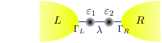
An important species of nanodevice is the double quantum dot (DQD) nanojunction, illustrated schematically in Fig. 1. Quantum dot and DQD semiconductor structures find many uses in quantum information processing, as they can be used to create charge Petta et al. (2004); Gorman et al. (2005); Nielsen et al. (2013); Scarlino et al. (2022) and spin Petta et al. (2005); Hanson et al. (2007); Fernández-Fernández et al. (2022); Burkard et al. (2023) qubits with long coherence times, making them ideal hardware for quantum computing implementations.
Nanoelectronic systems like the DQD nanojunction are well-described by the nonequilibrium Green’s function (NEGF) technique, an established method for describing quantum transport Ridley et al. (2022). In particular, the NEGF method provides access to conductance properties Wang et al. (1999), time-dependent currents You et al. (2000); Tuovinen et al. (2013), finite temperature effects Bâldea (2024) and shot noise Ridley et al. (2017), as well as higher moments of the full counting statistics Tang and Wang (2014) in response to a perturbation driving the system out of equilibrium.
In the general case, the NEGF approach can simultaneously deal with strong external fields, many-particle interactions, and transient effects for various quantum-transport setups Ridley et al. (2022); Tang and Wang (2024). While the drawback of this approach resides in the computational effort for solving the dynamical equations of motion, an accurate but computationally tractable scheme can be formulated in terms of the generalized Kadanoff-Baym ansatz Lipavský et al. (1986); Latini et al. (2014); Tuovinen et al. (2021). Recently, it has been established that this reconstruction results in a time-linear computational scheme for electron-electron Schlünzen et al. (2020); Joost et al. (2020), electron-boson Karlsson et al. (2021); Tuovinen and Pavlyukh (2024), and embedding effects Tuovinen et al. (2023); Pavlyukh et al. (2024); Cosco et al. (2024). However, in many experimentally and technologically relevant settings involving nanojunctions, a noninteracting approach can be sufficient Dutta et al. (2020); Ojajärvi et al. (2022); Ryu et al. (2022).
A recent development of an NEGF-based approach, the so-called time-dependent Landauer-Büttiker (TD-LB) formalism Stefanucci and Van Leeuwen (2013); Tuovinen et al. (2013, 2014); Ridley et al. (2015, 2016b); Ridley and Tuovinen (2018); Ridley et al. (2022), has been found to yield exact expressions for the time-dependent currents and noise in nanojunctions of arbitrary size, temperature and any time-dependent driving fields. In addition, this formalism incorporates the partition-free approach Stefanucci and Almbladh (2004); Ridley and Tuovinen (2018), where the lead-molecule coupling is present in the Hamiltonian at equilibrium, prior to the switch-on of a bias. The partition-free approach thus gives a more experimentally realizable description of the transient regime following a voltage quench in the nanojunction. The partition-free TD-LB methodology has recently been applied to superconducting nanowires Tuovinen et al. (2016, 2019), graphene nanoribbon structures Ridley and Tuovinen (2017); Ridley et al. (2019) and the local radiation profiles of molecular junctions Ridley et al. (2021). In addition, the TD-LB was used to study the problem of a driving field with a stochastic component in Ref. Ridley et al., 2016a, in which a quantum version of the classical Nyquist theorem relating conductance to the field fluctuations and temperature was derived.
In this work, we apply the TD-LB approach to the study of SR in a periodically driven nanojunction. The paper is structured as follows. In Section II.1, we outline the quantum transport setup for a nanojunction driven by biharmonic and Gaussian stochastic bias contributions. Section II.2 contains the main equations of the TD-LB formalism for an arbitrary time-dependent bias, supported by the underlying NEGF theory. In Section II.3, the resulting current formulas, following an averaging procedure over the stochastic bias, are expressed in a computationally tractable form in which all time and frequency integrals are calculated analytically yielding the current expression in a closed form via sums of special functions. The resulting expression is then averaged over a period of the driving field to give the net pump current across the nanojunction. The corresponding adiabatic limit is considered explicitly for the case of a quantum dot junction subject to a white noise bias. In Section III, numerical results are presented for the DQD system shown in Fig. 1. The main findings are: the fluctuation-dependence of current-voltage characteristics for the static bias case; the activation of photon-assisted SR; and the effects of particle-hole symmetry-breaking and color noise on the SR phenomenon. Finally, in Section IV we conclude and provide an outlook.
II Model and method
II.1 Quantum transport setup
For a typical set-up of a quantum transport problem shown in Fig. 1, we use the following Hamiltonian:
| (1) |
where is a time parameter on a contour, which is addressed in more detail in Sec. II.2. In Eq. (II.1), the first term corresponds to the sum of the Hamiltonians of the reservoirs/leads, where labels the leads, and labels the -th eigenstate of a lead. The second term corresponds to the Hamiltonian of the central region (the DQD in our case) and hence refers to electron hopping events within this region with indices and labeling localised orbitals there. Finally, the third term describes the coupling of the leads and the central system with the corresponding matrix elements , and denotes the spin degree of freedom of the electrons. Correspondingly, , and , are destruction and creation operators of the leads and the central system. Note that there is no direct interaction between the leads.
The system is driven out of equilibrium by the switch-on of a spatially uniform bias in each reservoir, modifying their energy dispersion . We assume this bias to be broken up into a constant shift , a deterministic time-dependent driving
| (2) |
chosen in the biharmonic form, and a stochastic time-dependent field leading to the full time-dependent bias being
| (3) |
The bias voltage protocol could be realized by an external electromagnetic field, and from now on it will be generally referred to as “photon-assisted” driving. We further assume that is a zero-mean, stationary, Gaussian stochastic process, uniform across the leads so that we can drop the index . The Gaussian nature of the noise means that odd-ordered statistical moments vanish, while even-ordered moments can be decomposed into a sum of products of pair correlation functions:
| (4) |
| (5) |
| (6) |
| (7) |
where we introduced a bias correlation function , denotes a summation over all permutations of pairs of the time variables, and the bar denotes the average taken with respect to the stochastic distribution of the bias. In analogy with classical approaches Pottier (2009), we choose a special form of the correlation function which involves a parameter , defining a finite correlation time , over which the bias is statistically correlated:
| (8) |
where is a parameter measuring the overall magnitude of bias fluctuations, such that . One intuitively expects an increase in to increase the dissipation and dephasing of molecular eigenmodes, as was discussed previously in Ref. Ridley et al., 2016a.
II.2 Time-dependent Landauer-Büttiker formalism
Based on the solution to the Kadanoff-Baym equations Kadanoff and Baym (1962), the NEGF technique provides formally exact access to the one-particle Green’s function
| (9) |
where the are fermionic field operators and denotes the Hamiltonian defined with respect to time variables on the Konstantinov-Perel’ time contour broken into (running from to ), (running backwards from to ) and (running from to , where is the inverse temperature) Konstantinov and Perel (1960); Keldysh (1964); Stefanucci and Van Leeuwen (2013). The variables correspond to spacetime locations with and being the spatial variable including the spin.
We collect the elements of the Hamiltonian Eq. (II.1) into the block matrix . A full description of the dynamics subsequent to the bias switch-on requires a specification of at every contour time :
| (10) | ||||
| (11) | ||||
| (12) |
where is the chemical potential and refers to the central region.
The Green’s function in Eq. (9) is projected onto the central (molecular) region to obtain the matrix-valued function , which satisfies the Kadanoff-Baym integro-differential equations of motion Stefanucci and Van Leeuwen (2013)
| (13) | |||
| (14) |
with the integral kernel given by the embedding self-energy
| (15) |
where is the Green’s function of the decoupled lead . Eqs. (13) and (14) are then projected onto equations for different components of the Green’s function (corresponding to different combinations of pairs of contour branch times) using the Langreth rulesLangreth (1976).
We now assume that the leads satisfy the wide-band limit approximation (WBLA), i.e. we neglect the energy dependence of the lead-molecule coupling. This assumption enables us to write down all components of the effective embedding self-energy in terms of the energy-independent level-width matrix
| (16) |
where is the equilibrium Fermi energy of lead . Within the WBLA, Eqs. (13) and (14) are linearized in terms of the effective Hamiltonian of the central region, . All components of the Green’s function can be calculated exactly in the two-time plane Ridley et al. (2015, 2016a). These Green’s function components and the corresponding embedding self-energy components are listed in Appendix A.
The quantum statistical expectation value of the current operator is given by
| (17) |
where and correspond to real and imaginary time convolutions Stefanucci and Van Leeuwen (2013). Setting the electronic charge and using the derived formulae for the components of in the WBLA, Eq. (17) can be shown to take the form Ridley et al. (2017):
| (18) |
where is the Fermi-Dirac distribution, and we have introduced the matrix
| (19) |
defined in terms of the retarded Green’s function . In Eq. (19), we also introduced the bias-voltage phase factor
| (20) |
It is essential that the bias enters only into these phase factors; hence, all the time information of the bias, including its stochastic part, is contained exclusively in exponential functions that appear linearly everywhere in the current expression.
Eq. (18) is a generalization of the well-known Landauer (1957); Büttiker (1986) Landauer-Büttiker formula for the current to include transient effects due to the partition-free quench, and due to an arbitrary time-dependent bias. We also note that the currents in the leads obey the following time-dependent continuity equation Ridley et al. (2016b)
| (21) |
where is the particle number in the central region and the lesser Green’s function is given in Eq. (40).
II.3 Noise-averaging and pump current
For the practical purposes of calculating the current in Eq. (18), it is advantageous to analytically calculate all frequency and time integrals to express the current in terms of special functions. In addition, one has to sample the current over the Gaussian fluctuations of the bias. The bias-voltage phase factors appearing in Eq. (18) may be decomposed into a product of terms with stochastic and biharmonic origin. Because the bias voltage appears only in the exponent, its averaging over the stochastic part of the bias can be done analytically using the fact that the average of the stochastic phase factor over a Gaussian noise is given by
| (22) |
so that we can insert here the color noise correlation function from Eq. (8) and expand this with respect to the stochastic bias in powers of , as was done in Ref. Ridley et al., 2016a. We note that dealing with the stochastic contribution to the bias in this way removes the need to sample over multiple stochastic trajectories and therefore drastically reduces the computational cost associated with the noisy bias. In addition, we expand the exponentiated harmonic terms via Bessel functions of the first kind Ridley et al. (2016a); Ridley and Tuovinen (2017), so that phase factors in Eq. (18) are replaced by:
| (23) |
where
| (24) |
These may be inserted into the expanded version of Eq. (18)
| (25) |
to give the full time-dependence of the current due to the stochastic and periodic fields. The complete expression for this is given as Eq. (53) in Appendix B, where all frequency integrals are replaced with summations over Matsubara frequencies and we also expand in terms of the left and right eigenvectors of the effective Hamiltonian :
| (26) |
Thus, the time-integrals appearing in Eq. (II.3) can be carried out analytically, as demonstrated in Appendix B.
The white noise case is recovered in the limit of zero correlation time ; in this limit only the term survives in the expansion (II.3) of the stochastic terms, which come in powers of the quantity . After taking the long time limit, transient modes are lost and we obtain the bias-averaged current:
| (27) |
where
| (28) |
Here, we have introduced the digamma function as the logarithmic derivative of the gamma function, .
For a consistency check, we may look at the static limit, , for all . In this case, only the summation terms survive, since the Bessel function satisfies for and at all other natural . Using properties of the left/right eigenvectors, one can then obtain the adiabatic limit of Eq. (27):
| (29) |
This is none other than the derived expression (C6) in Ref. Ridley et al., 2016a in the static bias case. We note that all time dependence has vanished. Eq. (29) defines a quantum fluctuation-dissipation relation for the nanojunction, as it relates conductance/resistance to temperature and fluctuation strength Pottier (2009); Ridley et al. (2016a).
Returning to Eq. (27), we assume that the frequency of driving is lead-independent, for all . This defines a driving period for the system. The difference of the currents between any two leads is then time-averaged over the period of to get the noise-affected quantum pump current in the steady-state:
| (30) |
where the appearing in the integral limits is an arbitrary time. We note that the net current between leads and is computed here because it corresponds to the average DC quantity measured in a real experiment Kohler et al. (2005). It must also be emphasized that the ‘pump’ terminology only applies to the case where the bias across the leads is zero on average. Since the first moment of the noisy bias is set to zero [Eq. (4)], and the biharmonic terms are zero under the time average, this condition is satisfied when the constant shifts , are equal.
For simplicity, we specialize now to the two-lead terminal, and label left and right leads by and , respectively. We also assume that the amplitudes of driving are independent of the lead, and . This leads to the stochastic bias-averaged quantum pump current
| (31) |
where we have defined the modified Kronecker delta function:
| (32) |
For evaluating Eq. (31), it is important to note that grows in the slow-driving () regime, approaching the adiabatic limit in Eq. (29) and may require a large number of Bessel function components for convergence. In the white noise regime (), bias fluctuations are small relative to the correlation frequency, so the stochastic-component summations converge fast. In the color noise regime (), more stochastic components may be required to achieve convergence.
Formula (31) reduces to Eq. (23) in Ref. Ridley and Tuovinen, 2017 in the limit of zero stochastic field () and equal biases . It enables us to compute the interplay of the color noise with the external driving field. We finally note that charge is conserved across the nanojunction in the case of the driving bias considered here, i.e.
| (33) |
by the continuity Eq. (21) and by the linearity of the bias-averaging, time averaging and time derivative operations.
III Results
III.1 Single-level molecular region
In order to fix physical ideas, we first specialize the discussion to the case of a single level molecular region (the quantum dot case). In this case, the effective Hamiltonian is a scalar, where is the on-site dot energy and is the scalar level width for the two-lead model. We also set the chemical potential for simplicity of notation.
We consider the case, also considered in Ref. Ridley et al., 2016a where there is no periodic driving. For simplicity, we also assume that the correlation frequency (the white noise case), and we also take the zero temperature limit . The bias is assumed to be applied symmetrically across the leads, such that . In this case, the bias-averaged current reduces to
| (34) |
from which the differential conductance can be extracted:
| (35) |
Note that in the limit of large fluctuations, , the conductance becomes independent of the voltage . This defines the ohmic regime Ridley et al. (2016a). From Eq. (III.1) we state a precise condition for stochastic enhancement of the conductance by the driving field, i.e. when the parameter set satisfies
| (36) |
In the limit of large bias , condition Eq. (36) is equivalent to , which is always satisfied. However, in this latter regime, the conductance tends to zero.
In general, we should therefore explore an intermediate parameter range in which there is a finite enhancement of a finite conductance due to the presence of the stochastic field.
III.2 DQD molecular junction
We now study numerically the double quantum dot (DQD) system shown in Fig. 1, with onsite dot energies , , inter-dot coupling parameter and coupling to the left and right leads described by the level broadening , respectively, within the WBLA. The effective model Hamiltonian for the central molecular region is thus given by
| (37) |
which determines the left/right eigenvalues/eigenvectors in Eq. (26). It is seen that the state is coupled to the left lead, while the state to the right. Since we want to focus on the effect of the bias fluctuations, we simplify by considering the equal coupling to the leads, , and then concentrate on the weak-coupling regime using , where the WBLA is known to be accurate Verzijl et al. (2013); Covito et al. (2018). Qualitatively, stronger coupling results in more broadened spectral features, cf. Eq. (III.1).
III.3 Stochastic field with constant driving
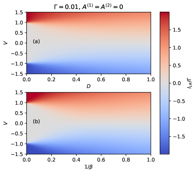
We first consider the case with no time-periodic driving term in the lead bias and , in the white noise case and with the DQD Hamiltonian parameterized by and . Fig. 2(a) displays the steady-state current-voltage characteristics as a function of the stochastic parameter , at zero temperature. We see a transition from the step-like current-voltage characteristics to a linear, ohmic dependence of the current on the voltage with increasing . This is compared to the case of zero fluctuations and varying temperature in Fig. 2(b), from which it is apparent that the effect of the environmental fluctuations on the current is qualitatively identical to that of temperature. We note that this is not true for all variables: the temperature and the environmental fluctuations can have qualitatively different effects on the current noise Moskalets and Haack (2016). We also note that, for this case of a static bias plus white noise, the results of computing Eq. (31) are identical to those obtained from the adiabatic limit in Eq. (29), because in this limit the bias-averaged current exhibits no time-dependence.
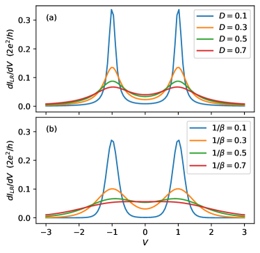
In Fig. 3, we show differential conductances in units of the conductance quantum , evaluated by numerical differentiation from the pump currents shown in Fig. 2, for different values of the fluctuation strength (panel a) and the temperature (panel b). Similar to the discussion of Fig. 2, we observe that the typical double-peak structure in the conductance is progressively smeared out as the fluctuation strength and temperature are increased.
III.4 Stochastic field with periodic driving
We now turn to the case of the periodically driven DQD. Fig. 4 illustrates the pump current as a function of the phase difference and the fluctuation strength , for different values of the static bias , see Eqs. (II.1) and (3): to better isolate the behavior of the stochastic drive, we fix the constant value of the bias to be equal on both left and right leads, so that applying a phase difference corresponds to the entirely antisymmetric bias window. Also, to simplify the large parameter space of the driving protocol, we set , take the modulating amplitudes as half the voltage shift, , and set first the driving frequency .
Interestingly, in the and cases [Figs. 4(a,c)], the pump current decays rapidly with increasing fluctuation strength. However, in the intermediate regime [Fig. 4(b)], we observe a clear stochastic enhancement of the pump current near . At zero fluctuations, a sizable pump current exists at the off-phase points in all cases. This arises because, even if the constant bias does not align with the resonant energy levels (the real parts of the eigenvalues of the matrix in Eq. (37)) of the DQD at , the modulating amplitudes generate a directed current Ridley and Tuovinen (2017). (Similarly, the in-phase points show diminishing pump currents in all cases.) However, the rectification effect is suppressed by bias fluctuations unless the constant bias aligns with the resonant levels (). When alignment occurs, fluctuations enhance rectification, leading to photon-assisted SR.
In Fig. 4, we also find that the pump current changes sign as the applied bias crosses the value related to the resonant energy levels of the DQD system [Figs. 4(a,c)]. This effect can be understood by photon-assisted electron and hole transfer processes Ridley and Tuovinen (2017); Ridley et al. (2022). The chemical potential of the coupled system is set in the middle of the DQD energy levels () indicating the corresponding electron populations in the leads. The effect is then seen as a directed current through the DQD from left to right (positive current) or opposite direction (negative current).
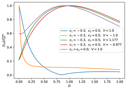
The parameter space of the driving protocol in Eq. (II.1) is very large. Since we are restricting the discussion on specific parameters, it is possible that there are more optimized settings for enhancing the SR effect even more. For this reason, we now refer to the situation in Fig. 4(b), and , as the ‘optimum SR’ scenario (within our parameter regime). In this situation, we analyze the impact of other parameters in the DQD junction. Fig. 5 illustrates the effect of on-site potentials in Eq. (37). These parameters can be tuned in practice using local gate voltages Hanson et al. (2007), which lift particle-hole degeneracy and shift the DQD resonant levels. For this, we set and which modifies the energy levels of from to . Applying the same static bias voltage profile, , that induces strong SR in Fig. 4, now results in a decaying behavior with increasing bias fluctuations. Note, however, the currents are not necessarily symmetric when mirroring the bias due to the broken particle-hole symmetry and the chemical potential being kept fixed at . Adjusting the constant bias to the modified resonant levels, or , restores the SR effect, demonstrating the robustness of SR against local fields that break particle-hole symmetry.
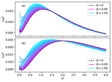
The position of the photon-assisted SR peak with respect to fluctuation strength depends on the driving frequency. Fig. 6(a) shows a frequency sweep within the white-noise regime (), still focusing on the optimal SR case and . (Also, the on-site potentials are again set to .) The SR peak shifts with driving frequency: a faster driving () causes SR at weaker fluctuations (), slower driving () requires stronger fluctuations () for SR, but eventually, all curves decay at large . We also observed (not shown) that beyond a threshold in increasing driving frequencies (), the system cannot respond fast enough, leading to monotonically decreasing current with . Fig. 6(b) shows the color-noise regime (), where the SR peak shifts to higher for both fast and slow driving. As decreases, the correlation time increases, resulting in a ‘smearing’ out of the SR peak due to an increased effective range of resonant bias values. The effect of the color noise is therefore to improve the stability of the transport signal against bias fluctuations.
Related to the convergence discussion after Eq. (31), here the most challenging case (, , ) requires Bessel function components and stochastic components for convergence. This calculation then involves about calls to the GSL special function library Galassi (2009).
The slow-driving regime can also be approached by employing the adiabatic limit in Eq. (29). In place of the constant shifts , , we insert a set of ‘time-dependent’ values from Eq. (II.1) into Eq. (29), and then average over one period of oscillation. While this procedure is not as general as the bias averaging carried out with Eq. (II.3), it is expected to provide the adiabatic limit, , for the AC-driven pump currents in the absence of a stochastic time-dependent fields, , without having to numerically converge a large number of Bessel function components Moskalets and Büttiker (2002); Moskalets (2011). This procedure happens to work in the presence of a stochastic noise as well. The result is shown as black dashed lines in Fig. 6. Importantly, we see the SR effect is clearly visible also in this case, practically coinciding with the cases. While the peak position changes with , the overall SR effect is not limited by this parameter, and could be detectable with state-of-the-art electronics operating at the terahertz regime Urteaga et al. (2017).
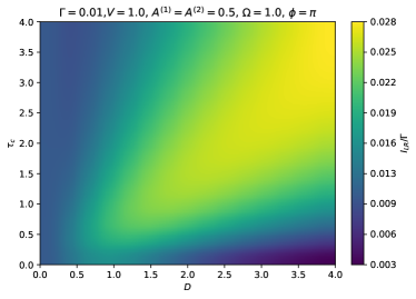
The shift of the SR peak between white- and color-noise regimes is further analyzed in Fig. 7 by varying both correlation time and the fluctuation strength while keeping the driving frequency fixed at . In addition, this calculation again focuses on the optimum SR case with and . The pump current maximum moves roughly diagonally in the -plane but becomes smeared at large as the DQD system operates through stronger bias fluctuations and color noise.
IV Conclusions
We have shown in this work that a nanojunction subject to a noisy external field can make positive use of the noise when assisted by a periodically-varying driving voltage. Furthermore, we have mapped out the parameter range in which this stochastic resonance effect is optimized for a double quantum dot nanojunction. To this end, we have generalized the time-dependent Landauer-Büttiker method to incorporate both stochastic and deterministic terms in the bias profile and have shown how the resulting non-linear time-dependent current response reduces to earlier results reported in the literature. This enabled us to optimize the stochastic resonance effect in the pumped electron current, and to demonstrate its dependence on intramolecular frequencies. In addition, we have computed the effect of varying the driving frequency and the fluctuation correlation time on SR, demonstrating its resilience across a wide range of parameter regimes. While we established how the SR depends on the frequency and fluctuations of the bias, we also confirmed the overall effect is present at the adiabatic limit, and could be observed with terahertz-scale electronics Urteaga et al. (2017).
In future work, we will investigate SR in more structurally diverse nanojunctions such as graphene nanoribbons, for which the validity of the TD-LB formalism is well-established Tuovinen et al. (2014); Gomes da Rocha et al. (2015); Ridley and Tuovinen (2017). We will also study the complex interplay between the timescales of the stochastic driving field, dissipation and driving time period, using Eqs. (27) and (53). The formalism developed here may also be extended to study SR in energy currents Covito et al. (2018), which will enable us to harness it for the optimization of thermoelectric effects. Finally, we may consider the effect of the noisy bias on the current-current correlations and quantum noise, using the formalism developed in Ref. Ridley et al., 2017. This will enable us to look at the effects of, e.g., noise on the electronic traversal time Ridley et al. (2019) in the context of transiently emerging topological phenomena in nanojunctions out of equilibrium Tuovinen et al. (2019); Barański et al. (2021); Tuovinen (2021); Górski et al. (2024).
Acknowledgements.
M.R. acknowledges support from the European Union’s Horizon Europe research and innovation programme under grant agreement No. 101178170. M.M. acknowledges the support from CSIC/IUCRAN2022 under Grant No. UCRAN20029. L.B. and R.T. acknowledge the EffQSim project funded by the Jane and Aatos Erkko Foundation. We also acknowledge grants of computer capacity from the Finnish Grid and Cloud Infrastructure (persistent identifier urn:nbn:fi:research-infras-2016072533).Appendix A Green’s function and self-energy components in the WBLA
In this section, we first list the Green’s function components for the generic time-dependent Hamiltonian studied in this paper [Eq. (II.1)]. These have been derived in previous works on the TD-LB formalism Stefanucci and Van Leeuwen (2013); Ridley et al. (2015, 2016a). In the arguments of these functions, we use the notation to denote real times taken on the horizontal branch of the Konstantinov-Perel’ contour, and denotes the imaginary part of taken on the Matsubara branch. The real-time components read:
| (38) |
| (39) |
| (40) |
Here, the matrix is defined in Eq. (19). The mixed and Matsubara components read:
| (41) |
| (42) |
| (43) |
Here we have defined the Matsubara frequencies , and the Fourier transformed Matsubara Green’s function
| (44) |
The corresponding embedding self-energy components are as follows:
| (45) |
| (46) |
| (47) |
| (48) |
| (49) |
In the latter expression, when and when .
Appendix B Full expansion of the bias-averaged current
The numerical results in this paper are obtained by analytically removing all time and frequency integrals in Eq. (II.3). The time integrals are removed by replacing all phase factors with the expansion in Eq. (II.3). The frequency integrals are removed by making use of the following simple pole expansion of the Fermi function:
| (50) |
where the are the so-called Matsubara frequencies Ridley and Tuovinen (2017). When Eq. (50) is inserted into Eq. (II.3), the resulting expression is given in terms of the digamma function, and the Hurwitz-Lerch transcendental function Hurwitz (1887); Lerch (1887), which is defined as follows:
| (51) |
For notational convenience, we also introduce the following compact object in terms of Eq. (51):
| (52) |
The expression which results from the removal of all integrals, although cumbersome, enables one to evaluate the current as a ‘single shot’ function of time:
| (53) |
where
| (54) |
| (55) |
and
| (56) |
where we have introduced the following shortcuts alongside the ones in Eqs. (24) and (28):
Taking the limit in which the initial condition is set to the infinite past, and swapping the indices , , one obtains the expression in Eq. (27).
References
- Gammaitoni et al. (1998) L. Gammaitoni, P. Hänggi, P. Jung, and F. Marchesoni, Reviews of modern physics 70, 223 (1998).
- Benzi et al. (1981) R. Benzi, A. Sutera, and A. Vulpiani, Journal of Physics A: mathematical and general 14, L453 (1981).
- Luchinsky et al. (1999) D. G. Luchinsky, R. Mannella, P. V. McClintock, and N. G. Stocks, IEEE Transactions on Circuits and Systems II: Analog and Digital Signal Processing 46, 1205 (1999).
- Harmer et al. (2002) G. P. Harmer, B. R. Davis, and D. Abbott, IEEE Transactions on Instrumentation and Measurement 51, 299 (2002).
- Mikhaylov et al. (2021) A. Mikhaylov, D. Guseinov, A. Belov, D. Korolev, V. Shishmakova, M. Koryazhkina, D. Filatov, O. Gorshkov, D. Maldonado, F. Alonso, et al., Chaos, Solitons & Fractals 144, 110723 (2021).
- Yilmaz et al. (2013) E. Yilmaz, M. Uzuntarla, M. Ozer, and M. Perc, Physica A: Statistical Mechanics and its Applications 392, 5735 (2013).
- Yamakou et al. (2020) M. E. Yamakou, P. G. Hjorth, and E. A. Martens, Frontiers in computational neuroscience 14, 62 (2020).
- Alley et al. (2001) R. Alley, S. Anandakrishnan, and a. P. Jung, Paleoceanography 16, 190 (2001).
- Ganopolski and Rahmstorf (2002) A. Ganopolski and S. Rahmstorf, Physical Review Letters 88, 038501 (2002).
- Douglass et al. (1993) J. K. Douglass, L. Wilkens, E. Pantazelou, and F. Moss, Nature 365, 337 (1993).
- Hänggi (2002) P. Hänggi, ChemPhysChem 3, 285 (2002).
- McDonnell and Abbott (2009) M. D. McDonnell and D. Abbott, PLoS computational biology 5, e1000348 (2009).
- Löfstedt and Coppersmith (1994) R. Löfstedt and S. Coppersmith, Physical review letters 72, 1947 (1994).
- Grifoni and Hänggi (1996) M. Grifoni and P. Hänggi, Physical review letters 76, 1611 (1996).
- Goychuk and Hänggi (1999) I. Goychuk and P. Hänggi, Physical Review E 59, 5137 (1999).
- Huelga and Plenio (2007) S. F. Huelga and M. B. Plenio, Physical review letters 98, 170601 (2007).
- Hänze et al. (2021) M. Hänze, G. McMurtrie, S. Baumann, L. Malavolti, S. N. Coppersmith, and S. Loth, Science advances 7, eabg2616 (2021).
- Li et al. (2024a) H. Li, K. Sun, and W. Yi, Physical Review Research 6, L042046 (2024a).
- Wagner et al. (2019) T. Wagner, P. Talkner, J. C. Bayer, E. P. Rugeramigabo, P. Hänggi, and R. J. Haug, Nature Physics 15, 330 (2019).
- German et al. (1994) A. German, V. Kovarskii, and N. Perel’Man, Zh. Eksp. Teor. Fiz 106, 801 (1994).
- Dykman et al. (1995) M. I. Dykman, T. Horita, and J. Ross, The Journal of chemical physics 103, 966 (1995).
- Astumian and Moss (1998) R. D. Astumian and F. Moss, Chaos: An Interdisciplinary Journal of Nonlinear Science 8, 533 (1998).
- Jiang et al. (2010) L.-L. Jiang, L. Huang, R. Yang, and Y.-C. Lai, Applied Physics Letters 96, 262114 (2010).
- Hartmann et al. (2010) F. Hartmann, D. Hartmann, P. Kowalzik, A. Forchel, L. Gammaitoni, and L. Worschech, Applied Physics Letters 96, 172110 (2010).
- Soni et al. (2010) R. Soni, P. Meuffels, A. Petraru, M. Weides, C. Kügeler, R. Waser, and H. Kohlstedt, Journal of applied physics 107, 024517 (2010).
- Bargueno et al. (2011) P. Bargueno, S. Miret-Artés, and I. Gonzalo, Physical chemistry chemical physics 13, 850 (2011).
- Hayashi et al. (2012) K. Hayashi, S. de Lorenzo, M. Manosas, J. Huguet, and F. Ritort, Physical Review X 2, 031012 (2012).
- Popescu et al. (2012) B. Popescu, P. B. Woiczikowski, M. Elstner, and U. Kleinekathöfer, Physical Review Letters 109, 176802 (2012).
- Hirano et al. (2013) Y. Hirano, Y. Segawa, T. Kawai, and T. Matsumoto, The Journal of Physical Chemistry C 117, 140 (2013).
- Brunner et al. (2014) J. Brunner, M. T. González, C. Schönenberger, and M. Calame, Journal of Physics: Condensed Matter 26, 474202 (2014).
- Pfeffer et al. (2015) P. Pfeffer, F. Hartmann, S. Höfling, M. Kamp, and L. Worschech, Physical Review Applied 4, 014011 (2015).
- Ridley et al. (2016a) M. Ridley, A. MacKinnon, and L. Kantorovich, Phys. Rev. B 93, 205408 (2016a).
- Gurvitz et al. (2016) S. Gurvitz, A. Aharony, and O. Entin-Wohlman, Physical Review B 94, 075437 (2016).
- Fujii et al. (2017) H. Fujii, A. Setiadi, Y. Kuwahara, and M. Akai-Kasaya, Applied Physics Letters 111, 133501 (2017).
- Entin-Wohlman et al. (2017) O. Entin-Wohlman, D. Chowdhury, A. Aharony, and S. Dattagupta, Physical Review B 96, 195435 (2017).
- Yoshida and Hirakawa (2017) K. Yoshida and K. Hirakawa, Nanotechnology 28, 125205 (2017).
- Kosov (2018) D. S. Kosov, The Journal of Chemical Physics 148, 184108 (2018).
- Aharony et al. (2019) A. Aharony, O. Entin-Wohlman, D. Chowdhury, and S. Dattagupta, Journal of Statistical Physics 175, 704 (2019).
- Hussein et al. (2020) R. Hussein, S. Kohler, J. C. Bayer, T. Wagner, and R. J. Haug, Physical Review Letters 125, 206801 (2020).
- Markina et al. (2020) A. Markina, A. Muratov, V. Petrovskyy, and V. Avetisov, Nanomaterials 10, 2519 (2020).
- Roldán et al. (2024) J. Roldán, A. Cantudo, J. Torres, D. Maldonado, Y. Shen, W. Zheng, Y. Yuan, and M. Lanza, npj 2D Materials and Applications 8, 7 (2024).
- Tao (2006) N. J. Tao, Nature nanotechnology 1, 173 (2006).
- Li et al. (2023) T. Li, V. K. Bandari, and O. G. Schmidt, Advanced Materials 35, 2209088 (2023).
- Yoshioka et al. (2016) K. Yoshioka, I. Katayama, Y. Minami, M. Kitajima, S. Yoshida, H. Shigekawa, and J. Takeda, Nature Photonics 10, 762 (2016).
- Garg and Kern (2020) M. Garg and K. Kern, Science 367, 411 (2020).
- Viti et al. (2020) L. Viti, A. R. Cadore, X. Yang, A. Vorobiev, J. E. Muench, K. Watanabe, T. Taniguchi, J. Stake, A. C. Ferrari, and M. S. Vitiello, Nanophotonics 10, 89 (2020).
- Qiu and Huang (2021) Q. Qiu and Z. Huang, Advanced Materials 33, 2008126 (2021).
- Leitenstorfer et al. (2023) A. Leitenstorfer, A. S. Moskalenko, T. Kampfrath, J. Kono, E. Castro-Camus, K. Peng, N. Qureshi, D. Turchinovich, K. Tanaka, A. G. Markelz, et al., Journal of Physics D: Applied Physics 56, 223001 (2023).
- Li et al. (2024b) R. Li, H. Li, X. Zhang, B. Liu, B. Wu, B. Zhu, J. Yu, G. Liu, L. Zheng, and Q. Zeng, Advanced Functional Materials 34, 2402797 (2024b).
- Sun et al. (2024) X. Sun, R. Liu, S. Kandapal, and B. Xu, Nanophotonics 13, 1535 (2024).
- Moskalets and Büttiker (2002) M. Moskalets and M. Büttiker, Physical Review B 66, 205320 (2002).
- Arrachea and Moskalets (2006) L. Arrachea and M. Moskalets, Physical Review B—Condensed Matter and Materials Physics 74, 245322 (2006).
- Iurov et al. (2011) A. Iurov, G. Gumbs, O. Roslyak, and D. Huang, Journal of Physics: Condensed Matter 24, 015303 (2011).
- Moskalets (2011) M. V. Moskalets, Scattering matrix approach to non-stationary quantum transport (World Scientific, 2011).
- Ridley and Tuovinen (2017) M. Ridley and R. Tuovinen, Physical Review B 96, 195429 (2017), publisher: APS.
- Petta et al. (2004) J. Petta, A. Johnson, C. Marcus, M. Hanson, and A. Gossard, Physical review letters 93, 186802 (2004).
- Gorman et al. (2005) J. Gorman, D. Hasko, and D. Williams, Physical review letters 95, 090502 (2005).
- Nielsen et al. (2013) E. Nielsen, E. Barnes, J. Kestner, and S. Das Sarma, Physical Review B—Condensed Matter and Materials Physics 88, 195131 (2013).
- Scarlino et al. (2022) P. Scarlino, J. H. Ungerer, D. J. van Woerkom, M. Mancini, P. Stano, C. Müller, A. J. Landig, J. V. Koski, C. Reichl, W. Wegscheider, et al., Physical Review X 12, 031004 (2022).
- Petta et al. (2005) J. R. Petta, A. C. Johnson, J. M. Taylor, E. A. Laird, A. Yacoby, M. D. Lukin, C. M. Marcus, M. P. Hanson, and A. C. Gossard, Science 309, 2180 (2005).
- Hanson et al. (2007) R. Hanson, L. P. Kouwenhoven, J. R. Petta, S. Tarucha, and L. M. K. Vandersypen, Rev. Mod. Phys. 79, 1217 (2007).
- Fernández-Fernández et al. (2022) D. Fernández-Fernández, Y. Ban, and G. Platero, Physical Review Applied 18, 054090 (2022).
- Burkard et al. (2023) G. Burkard, T. D. Ladd, A. Pan, J. M. Nichol, and J. R. Petta, Reviews of Modern Physics 95, 025003 (2023).
- Ridley et al. (2022) M. Ridley, N. W. Talarico, D. Karlsson, N. L. Gullo, and R. Tuovinen, Journal of Physics A: Mathematical and Theoretical 55, 273001 (2022).
- Wang et al. (1999) B. Wang, J. Wang, and H. Guo, Physical review letters 82, 398 (1999).
- You et al. (2000) J. You, C.-H. Lam, and H. Zheng, Physical Review B 62, 1978 (2000).
- Tuovinen et al. (2013) R. Tuovinen, R. van Leeuwen, E. Perfetto, and G. Stefanucci, J. Phys.: Conf. Ser. 427, 012014 (2013).
- Bâldea (2024) I. Bâldea, Physical Chemistry Chemical Physics 26, 6540 (2024).
- Ridley et al. (2017) M. Ridley, A. MacKinnon, and L. Kantorovich, Phys. Rev. B 95, 165440 (2017).
- Tang and Wang (2014) G.-M. Tang and J. Wang, Phys. Rev. B 90, 195422 (2014).
- Tang and Wang (2024) G. Tang and J.-S. Wang, Physical Review B 109, 085428 (2024).
- Lipavský et al. (1986) P. Lipavský, V. Špička, and B. Velický, Phys. Rev. B 34, 6933 (1986).
- Latini et al. (2014) S. Latini, E. Perfetto, A.-M. Uimonen, R. van Leeuwen, and G. Stefanucci, Phys. Rev. B 89, 075306 (2014).
- Tuovinen et al. (2021) R. Tuovinen, R. van Leeuwen, E. Perfetto, and G. Stefanucci, The Journal of Chemical Physics 154, 094104 (2021).
- Schlünzen et al. (2020) N. Schlünzen, J.-P. Joost, and M. Bonitz, Phys. Rev. Lett. 124, 076601 (2020).
- Joost et al. (2020) J.-P. Joost, N. Schlünzen, and M. Bonitz, Phys. Rev. B 101, 245101 (2020).
- Karlsson et al. (2021) D. Karlsson, R. van Leeuwen, Y. Pavlyukh, E. Perfetto, and G. Stefanucci, Phys. Rev. Lett. 127, 036402 (2021).
- Tuovinen and Pavlyukh (2024) R. Tuovinen and Y. Pavlyukh, Nano Letters 24, 9096 (2024).
- Tuovinen et al. (2023) R. Tuovinen, Y. Pavlyukh, E. Perfetto, and G. Stefanucci, Phys. Rev. Lett. 130, 246301 (2023).
- Pavlyukh et al. (2024) Y. Pavlyukh, R. Tuovinen, E. Perfetto, and G. Stefanucci, Phys. Status Solidi B 261, 2300504 (2024).
- Cosco et al. (2024) F. Cosco, R. Tuovinen, and N. Lo Gullo, Phys. Status Solidi B 261, 2300561 (2024).
- Dutta et al. (2020) B. Dutta, D. Majidi, N. W. Talarico, N. Lo Gullo, H. Courtois, and C. B. Winkelmann, Phys. Rev. Lett. 125, 237701 (2020).
- Ojajärvi et al. (2022) R. Ojajärvi, F. S. Bergeret, M. A. Silaev, and T. T. Heikkilä, Phys. Rev. Lett. 128, 167701 (2022).
- Ryu et al. (2022) S. Ryu, R. López, L. Serra, and D. Sánchez, Nature Communications 13, 2512 (2022).
- Stefanucci and Van Leeuwen (2013) G. Stefanucci and R. Van Leeuwen, Nonequilibrium many-body theory of quantum systems: a modern introduction (Cambridge University Press, 2013).
- Tuovinen et al. (2014) R. Tuovinen, E. Perfetto, G. Stefanucci, and R. van Leeuwen, Phys. Rev. B 89, 085131 (2014).
- Ridley et al. (2015) M. Ridley, A. MacKinnon, and L. Kantorovich, Phys. Rev. B 91, 125433 (2015).
- Ridley et al. (2016b) M. Ridley, A. MacKinnon, and L. Kantorovich, J. Phys.: Conf. Ser. 696, 012017 (2016b).
- Ridley and Tuovinen (2018) M. Ridley and R. Tuovinen, J Low Temp Phys 191, 380 (2018).
- Stefanucci and Almbladh (2004) G. Stefanucci and C.-O. Almbladh, Physical Review B 69, 195318 (2004).
- Tuovinen et al. (2016) R. Tuovinen, R. van Leeuwen, E. Perfetto, and G. Stefanucci, J. Phys.: Conf. Ser. 696, 012016 (2016).
- Tuovinen et al. (2019) R. Tuovinen, E. Perfetto, R. v. Leeuwen, G. Stefanucci, and M. A. Sentef, New J. Phys. 21, 103038 (2019).
- Ridley et al. (2019) M. Ridley, M. A. Sentef, and R. Tuovinen, Entropy 21, 737 (2019).
- Ridley et al. (2021) M. Ridley, L. Kantorovich, R. van Leeuwen, and R. Tuovinen, Physical Review B 103, 115439 (2021), publisher: APS.
- Pottier (2009) N. Pottier, Nonequilibrium statistical physics: linear irreversible processes (Oxford University Press, 2009).
- Kadanoff and Baym (1962) L. P. Kadanoff and G. A. Baym, Quantum Statistical Mechanics Green’s Function Methods in Equilibrium Problems (Benjamin, 1962).
- Konstantinov and Perel (1960) O. Konstantinov and V. Perel, Zhur. Eksptl’. i Teoret. Fiz. 39 (1960), publisher: Leningrad Inst. of Physics and Tech.
- Keldysh (1964) L. Keldysh, Zh. Eksp. Teor. Fiz. 47, 1515 (1964).
- Langreth (1976) D. C. Langreth, in Linear and nonlinear electron transport in solids (Springer, 1976) pp. 3–32.
- Landauer (1957) R. Landauer, IBM Journal of research and development 1, 223 (1957).
- Büttiker (1986) M. Büttiker, Physical review letters 57, 1761 (1986).
- Kohler et al. (2005) S. Kohler, J. Lehmann, and P. Hänggi, Physics Reports 406, 379 (2005).
- Verzijl et al. (2013) C. J. O. Verzijl, J. S. Seldenthuis, and J. M. Thijssen, The Journal of Chemical Physics 138, 094102 (2013).
- Covito et al. (2018) F. Covito, F. G. Eich, R. Tuovinen, M. A. Sentef, and A. Rubio, J. Chem. Theory Comput. 14, 2495 (2018).
- Moskalets and Haack (2016) M. Moskalets and G. Haack, Physica E: Low-dimensional Systems and Nanostructures 75, 358–369 (2016).
- Galassi (2009) M. Galassi, “GNU Scientific Library Reference Manual,” (2009), http://www.gnu.org/software/gsl.
- Urteaga et al. (2017) M. Urteaga, Z. Griffith, M. Seo, J. Hacker, and M. J. W. Rodwell, Proceedings of the IEEE 105, 1051 (2017).
- Gomes da Rocha et al. (2015) C. Gomes da Rocha, R. Tuovinen, R. van Leeuwen, and P. Koskinen, Nanoscale 7, 8627 (2015).
- Barański et al. (2021) J. Barański, M. Barańska, T. Zienkiewicz, R. Taranko, and T. Domański, Phys. Rev. B 103, 235416 (2021).
- Tuovinen (2021) R. Tuovinen, New Journal of Physics 23, 083024 (2021).
- Górski et al. (2024) G. Górski, K. P. Wójcik, J. Barański, I. Weymann, and T. Domański, Scientific Reports 14, 13848 (2024).
- Hurwitz (1887) A. Hurwitz, Zeitschrift für Math. und Physik 27, 86 (1887).
- Lerch (1887) M. Lerch, Acta math 11, 19 (1887).