ThriftLLM: On Cost-Effective Selection of Large Language Models for Classification Queries

Abstract.

In recent years, large language models (LLMs) have demonstrated remarkable capabilities in comprehending and generating natural language content, attracting widespread attention in both industry and academia. An increasing number of services offer LLMs for various tasks via APIs. Different LLMs demonstrate expertise in different domains of queries (e.g., text classification queries). Meanwhile, LLMs of different scales, complexity, and performance are priced diversely. Driven by this, several researchers are investigating strategies for selecting an ensemble of LLMs, aiming to decrease overall usage costs while enhancing performance. However, to the best of our knowledge, none of the existing works addresses the problem, how to find an LLM ensemble subject to a cost budget, which maximizes the ensemble performance with guarantees.

In this paper, we formalize the performance of an ensemble of models (LLMs) using the notion of prediction accuracy which we formally define. We develop an approach for aggregating responses from multiple LLMs to enhance ensemble performance. Building on this, we formulate the Optimal Ensemble Selection problem of selecting a set of LLMs subject to a cost budget that maximizes the overall prediction accuracy. We show that prediction accuracy is non-decreasing and non-submodular and provide evidence that the Optimal Ensemble Selection problem is likely to be NP-hard. By leveraging a submodular function that upper bounds prediction accuracy, we develop an algorithm called ThriftLLM and prove that it achieves an instance-dependent approximation guarantee with high probability. In addition, it achieves state-of-the-art performance for text classification and entity matching queries on multiple real-world datasets against various baselines in our extensive experimental evaluation, while using a relatively lower cost budget, strongly supporting the effectiveness and superiority of our method.

1. Introduction

The evolution of large language models (LLMs) in recent years has significantly transformed the field of natural language processing. These models have enabled AI systems to generate human-like texts based on input instructions with remarkable accuracy. An increasing number of companies (e.g., OpenAI, Anthropic, and Google) have introduced a wide range of services powered by LLMs, such as GPT-4 (OpenAI, 2023), Claude-3 (Anthropic, 2024), and Gemini (Gemini Team et al., 2023). These services, accessible via APIs, have achieved notable success across various applications, such as text classification, question answering, summarization, and natural language inference (Sun et al., 2023; Lei et al., 2023; Su et al., 2019; Zhang et al., 2024a). In data management, various LLMs have been adopted for text-to-SQL generation (Zhang et al., 2024b; Gao et al., 2024; Fan et al., 2024), query performance optimization (Trummer, 2024; Zhu et al., 2024; Wang et al., 2024), schema matching (Parciak et al., 2024), and entity matching (O’Reilly-Morgan et al., 2025; Peeters et al., 2025; Li et al., 2020).

While these models offer significant improvements in performance, they come with substantial costs, particularly for high-throughput applications. For example, GPT-4 charges $\$30$ per million input tokens and $\$60$ per million output tokens (help.openai.com, 2024), while Gemini-1.5 (livechatai.com, 2024) costs $\$7$ and $\$21$ per million input and output tokens, respectively. Typically, models with higher performance charge a higher price. However, it is well recognized that expensive models with larger number of parameters do not necessarily dominate the cheaper models across all applications (Chen et al., 2023; Chen and Li, 2024b; Xia et al., 2024; Shekhar et al., 2024; Sun et al., 2024). Different models may excel in different domains, and it has been observed that smaller LLMs can surpass larger LLMs on specific tasks (Chen et al., 2023; Fu et al., 2024; Ding et al., 2024).

This phenomenon raises an important question: can we leverage a set of cost-effective LLMs, within a specified budget, to achieve performance comparable to that of a more expensive LLM? The literature offers two main strategies to address this: LLM ensemble (Chen et al., 2023; Jiang et al., 2023; Shekhar et al., 2024) and tiny LM (Hillier et al., 2024; Chen and Varoquaux, 2024; Tang et al., 2024). The ensemble approach aims to optimize performance by combining outputs from a carefully selected set of LLMs. In contrast, the tiny LM approach applies advanced techniques to reduce the parameter counts of models without significantly compromising the performance. Specifically, FrugalGPT (Chen et al., 2023), a recent LLM ensemble work, derives an LLM cascade from a ground set optimized for given queries under a cost budget constraint. As a representative from the tiny LM family, Octopus v2 (Chen and Li, 2024a) fine-tunes the small model Gemma-2B to exploit fine-tuned functional tokens for function calling, achieving comparable performance with GPT-4 in accuracy and latency. Among the frameworks for LLM usage cost reduction and LLM performance enhancement, FrugalGPT is the most pertinent to our research. However, when FrugalGPT applies the derived LLM cascade to queries, it adopts the single output from the last executed model in the sequence rather than taking advantage of all generated responses from the model cascade to produce an optimal solution. Moreover, the budget constraint is applied to queries in an expected sense, allowing the incurred costs on individual queries to exceed the budget in practice, a phenomenon confirmed by our experiments. In addition, FrugalGPT does not provide any performance guarantee for the selected LLM ensemble.

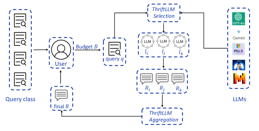
Figure 1. Overview of ThriftLLM: $R_{i},R_{j},R$ denote responses.

Inspired by these observations, we aim to combine the responses generated by a collection of LLMs in a non-trivial manner to deliver high-quality output, with a focus on classification queris. To this end, we devise a novel aggregation approach and quantify the quality of the aggregated response via a new metric of prediction accuracy by leveraging likelihood maximization. Building on this, we formalize an optimization problem, dubbed Optimal Ensemble Selection (OES for short): given a set of LLMs, a specific budget, and a query, the objective is to identify a subset of LLMs whose total cost is within the budget while the aggregated prediction accuracy on the query is maximized. To address this challenge, we propose an adaptive LLM selection algorithm ThriftLLM, designed specifically for this budget-constrained LLM selection scenario. As illustrated in Figure 1, when receiving a query and budget from a user, ThriftLLM selects an appropriate subset of LLMs from the LLM candidates without exceeding the budget. These LLMs independently process the query, and their responses are subsequently aggregated by ThriftLLM to produce a final answer of high quality, which is then returned to the user.

We conduct an in-depth theoretical analysis of the prediction accuracy function in the OES problem and establish that it is non-decreasing and non-submodular. We also provide evidence of the hardness of the problem. Nevertheless, we leverage a surrogate objective function that upper bounds the prediction accuracy, show that it is non-decreasing and submodular, and devise an algorithm for OES that achieves an instance-dependent approximation guarantee with high probability, when LLM success probabilities are known. We show how our algorithms and approximation guarantees can be extended to the case when the success probabilities are unknown and are estimated within confidence intervals. We compare ThriftLLM with $3$ baselines on $5$ real-world datasets on various text classification queries across different domains as well as with $2$ SOAT baselines across $5$ real-world datasets on entity matching queries. The experimental results strongly demonstrate the superior performance of ThriftLLM in terms of accuracy respecting cost budgets and delivering high-quality results under given budgets.

In sum, we make the following contributions.

• We propose a new aggregation scheme for combining individual LLM responses and formalize the ensemble prediction quality using a novel notion of prediction accuracy (Sections 2 and 3). We show that prediction accuracy is non-decreasing but non-submodular and offer evidence of hardness of the Optimal Ensemble Selection problem (Section 4.1).

• We develop a greedy algorithm, GreedyLLM, and show that it has an unbounded approximation factor. We then develop the ThriftLLM algorithm by leveraging a submodular upper bound function as a surrogate objective, and show that it offers an instance dependent approximation to the optimum with high probability (Sections 4.2-4.3). When the success probabilities are unknown and are estimated within confidence intervals, we can show data-dependent approximation guarantees (Section 4.4).

• We conduct extensive experiments on text classification tasks over $5$ real-world datasets across diverse domains against $3$ baselines and on entity matching over $5$ real-world datasets against $2$ baselines. Experiments show that ThriftLLM achieves comparable or superior performance on the tested datasets while respecting the minimum budget constraints (Section 6).

Related work is discussed in Section 5 while Section 7 summarizes the paper and discusses future work. Proofs of most of our technical results can be found in Appendix A.

Table 1. Frequently used notations

Notation	Description
$\mathcal{L},L,\mathcal{S}$	the set of LLMs, the set size, and a subset of $\mathcal{L}$, i.e., $|\mathcal{L}|=L$ and $\mathcal{S}\subseteq\mathcal{L}$
$\mathcal{Q},q$	the query class and one random query
$R(l)$	the response of model $l\in\mathcal{L}$
$\mathcal{C}=\{C_{1},\ldots,C_{K}\}$, $C_{q}$	the set of classes and the ground-truth class of query $q$ with $C_{q}\in\mathcal{C}$
$\mathcal{P}=\{p_{1},p_{2},\cdots,p_{L}\}$	the set of success probabilities of LLMs on a query class
$B$, $b$	the total budget and a model cost on a query
$\Omega,\phi$	the observation space of possible responses and a specific observation
$\xi(\cdot)$	the function of prediction accuracy
$f(C_{k}\mid\phi)$	the likelihood function of $C_{k}$ being the ground truth given observation $\phi$
$h(C_{k}\mid\phi)$	the belief function of the predicted class $C_{k}$ given observation $\phi$

2. Preliminaries

We denote matrices, vectors, and sets with bold uppercase letters (e.g., $\mathbf{T}$), bold lowercase letters (e.g., $\mathbf{x}$), and calligraphic letters (e.g., $\mathcal{S}$), respectively. The $i$-th row (resp. column) of matrix $\mathbf{T}$ is denoted $\mathbf{T}[i,\cdot]$ (resp. $\mathbf{T}[\cdot,i]$). We use $[n]$ to denote the set $\{1,2,\cdots,n\}$. Frequently used notations are summarized in Table 1.

We refer to textual tasks submitted to LLMs as queries. Queries typically contain contexts, called prompts, preceding the actual questions. In general, we assume queries include necessary prompts. Let $\mathcal{Q}$ be a query class representing a specific category of queries in the real world and $\mathcal{L}=\{l_{1},l_{2},\cdots,l_{L}\}$ be a set of distinct LLMs ($L>0$). Given a random query $q\in\mathcal{Q}$ (with its corresponding prompt), the query processing cost of a model consists of two components: the input and output costs, which are directly determined by the number of input and output tokens, respectively. We let $b_{i}(q)\in\mathbb{R}_{+}$ denote the total incurred cost of model $l_{i}$ for processing query $q$. When the model $l_{i}$ is deterministic, its cost $b_{i}(q)$ is solely determined by the query $q$. For simplicity, we refer to this cost as $b_{i}$ when the query is clear from the context. The performance of the models from $\mathcal{L}$ on the query class $\mathcal{Q}$ is represented by the set of success probabilities $\mathcal{P}=\{p_{1},p_{2},\cdots,p_{L}\}$, where each $p_{i}$ denotes the probability that the model $l_{i}$ generates a correct response to a query selected uniformly at random from $\mathcal{Q}$.

Specifically, for a classification query $q\in\mathcal{Q}$, let $\mathcal{C}=\{C_{1},\ldots,C_{K}\}$ denote the set of $K>0$ possible classes. When model $l_{i}\in\mathcal{L}$ is applied to query $q$, it returns a prediction response denoted $R(l_{i})\in\mathcal{C}$. For a subset $\mathcal{S}\subseteq\mathcal{L}$ of LLMs, their prediction responses yield an observation $\phi_{\mathcal{S}}=(R(l)\mid l\in\mathcal{S})$, a prediction sequence of the LLMs from $\mathcal{S}$. The set of all possible observations for $\mathcal{S}$ on the query class $\mathcal{Q}$ is termed as observation space $\Omega_{\mathcal{S}}$. We denote the prediction derived from observation $\phi_{\mathcal{S}}\in\Omega_{\mathcal{S}}$ as $C(\phi_{\mathcal{S}})$. The derivation procedure is elaborated in Section 3.2.

Given a set of LLMs $\mathcal{S}$ and considering a random query $q$ from $\mathcal{Q}$ with an associated ground-truth class $C_{q}$, the probability of observing $\phi_{\mathcal{S}}$, denoted as $Pr[\phi_{\mathcal{S}}]$, is computed as follows. Let $\mathcal{S}^{T}=\{l\in\mathcal{S}\mid R(l)=C_{q}\}$ (resp. $\mathcal{S}^{F}=\{l\in\mathcal{S}\mid R(l)\neq C_{q}\}$) be the subset of models whose prediction agrees (resp. disagrees) with $C_{q}$. Then $Pr[\phi_{\mathcal{S}}]$ is

(1) $$\textstyle Pr[\phi_{\mathcal{S}}]=\prod_{l_{i}\in\mathcal{S}^{T}}p_{i}\prod_{l_{j}\in\mathcal{S}_{F}}\tfrac{1-p_{j}}{K-1}.$$

Notice that a model making a wrong prediction could predict any one of the rest $K-1$ wrong classes. By leveraging the realization probability $Pr[\phi_{\mathcal{S}}]$, the fundamental concept prediction accuracy $\xi(\mathcal{S})$ of $\mathcal{S}$ with respect to the query class $\mathcal{Q}$ is formalized as follows.

Definition 0 (Prediction Accuracy).

Given a query $q$ sampled from class $\mathcal{Q}$ and a subset $\mathcal{S}$ of LLMs, let $C_{q}$ be the ground-truth response. Let $\Omega^{T}_{\mathcal{S}}\subset\Omega_{\mathcal{S}}$ be the subset of observations with $C(\phi_{\mathcal{S}})=C_{q}$. The prediction accuracy on query class $\mathcal{Q}$ is $\xi_{\mathcal{P}}(\mathcal{S})=\sum_{\phi_{\mathcal{S}}\in\Omega^{T}_{\mathcal{S}}}Pr[\phi_{\mathcal{S}}]$.

When the success probabilities $\mathcal{P}$ are clear from the context, we will drop the subscript and denote prediction accuracy as $\xi(.)$. We next formally state the problem we study in the paper.

Definition 0 (Optimal Ensemble Selection).

Consider a query class $\mathcal{Q}$, a set $\mathcal{L}$ of LLMs, and a cost budget $B\in\mathbb{R}_{+}$. The Optimal Ensemble Selection (OES) problem is to find a subset $\mathcal{S}^{\circ}\subseteq\mathcal{L}$ whose total cost is under $B$, such that the prediction accuracy $\xi(\mathcal{S}^{\circ})$ on $\mathcal{Q}$ is maximized, i.e.,

(2) $$\mathcal{S}^{\circ}=\underset{\mathcal{S}:\mathcal{S}\subseteq\mathcal{L},c(\mathcal{S})\leq B}{\operatorname{arg}\operatorname{max}}\;\xi(\mathcal{S}),$$

where $c(\mathcal{S}):=\sum_{l_{i}\in\mathcal{S}}b_{i}$ is the total cost of LLMs in $\mathcal{S}$.

3. Probability Estimation and Response Aggregation

A key ingredient in our optimization problem is the success probability of LLMs. In this section, we first discuss our approach for estimating the success probability of an LLM from historical data. We then elaborate on the methodology for deriving predictions based on observations. For ease of exposition, we assume the responses of different LLMs are mutually independent, and our analysis primarily concentrates on classification tasks.

3.1. Estimation of Success Probability

We assume that queries from the same query class $\mathcal{Q}$ exhibit semantic similarity. The success probability of a model $l$ on query class $\mathcal{Q}$ is the probability that $l$ returns the correct response for a query $q$ randomly sampled from $\mathcal{Q}$. This probability plays a crucial role in addressing the OES problem. However, success probabilities of LLMs are not known a priori but can be estimated from historical data.

Specifically, consider an input table $\mathbf{T}$ that records the historical performance of the $L$ LLMs on $N$ queries in a matrix format with $L,N\in\mathbb{N}_{+}$. The entries of the input table vary based on the type of query $q$. For classification tasks, table $\mathbf{T}$ contains boolean entries, i.e., $\mathbf{T}\in\{0,1\}^{N\times L}$. Conversely, for generation or regression tasks, it contains real values in the interval $[0,1]$, i.e., $\mathbf{T}\in[0,1]^{N\times L}$, with $\mathbf{T}_{\ell,k}$ indicating the quality or accuracy score of the response from the $\ell$-th model on the $k$-th query. In this paper, we focus on classification tasks.

To accurately estimate the success probability for each query class, we first cluster the queries in $\mathbf{T}$ into distinct groups based on their semantic similarity. To this end, we take advantage of embeddings to convert all queries into embeddings by leveraging the embedding API provided by OpenAI. Subsequently, we employ the DBSCAN (Gan and Tao, 2015) algorithm to cluster the embeddings. The success probability $p_{l}$ of the $l$-th model on the resultant cluster $\mathcal{Q}$ is estimated as $p_{l}=\tfrac{1}{|\mathcal{Q}|}\sum_{q_{i}\in\mathcal{Q}}\mathbf{T}[i,l]$.

3.2. Response Aggregation

Given a set $\mathcal{S}$ of LLMs and an observation $\phi_{\mathcal{S}}=(R(l_{1}),R(l_{2}),\cdots,R(l_{|\mathcal{S}|}))$, the aggregated prediction $C(\phi_{\mathcal{S}})$ of $\phi_{\mathcal{S}}$ is derived by combining all responses in observation $\phi_{\mathcal{S}}$. Since the ground-truth $C_{q}$ of query $q$ is unknown, we take the class with maximum likelihood as the aggregated prediction $C(\phi_{\mathcal{S}})$, as detailed below.

Specifically, each response in observation $\phi_{\mathcal{S}}$ corresponds to a class from $\mathcal{C}=\{C_{1},C_{2},\cdots,C_{K}\}$, in which one class represents the (unknown) ground truth $C_{q}$. We consider each of the $K$ classes in turn as the ground truth and compute the likelihood of observing $\phi_{\mathcal{S}}$. The class with the highest likelihood is selected as the prediction $C(\phi_{\mathcal{S}})$.

Initially, the set $\mathcal{S}$ is partitioned into disjoint subsets as $\mathcal{S}=\{\mathcal{S}(C_{1}),\mathcal{S}(C_{2}),\cdots,\mathcal{S}(C_{K})\}$ where $\mathcal{S}(C_{k})=\{l:R(l)=C_{k},l\in\mathcal{S}\}$ represents the subset of models that predicted class $C_{k}$. The likelihood function $f(C_{q}=C_{k}\mid\phi_{\mathcal{S}})$, which measures the probability of $C_{k}$ being the ground truth, is defined as

(3) $$\textstyle f(C_{q}=C_{k}\mid\phi_{\mathcal{S}})=\prod_{l_{i}\in\mathcal{S}(C_{k})}p_{i}\prod_{l_{j}\in\mathcal{S}\setminus\mathcal{S}(C_{k})}\tfrac{1-p_{j}}{K-1}$$

for $k\in[K]$. Based on this likelihood, we can derive the prediction $C(\phi_{\mathcal{S}})$ from observation $\phi_{\mathcal{S}}$ as $C(\phi_{\mathcal{S}})=\arg\max_{C_{k}\in\mathcal{C}}f(C_{q}=C_{k}\mid\phi_{\mathcal{S}})$. If there are multiple classes with the same maximal likelihood, we break the tie randomly.

Computing $f(C_{q}=C_{k}\mid\phi_{\mathcal{S}})$ for all $k\in[K]$ is expensive. However, by identifying redundant calculations, we can speed it up. Specifically, computing $f(.)$ involves a substantial amount of repeated calculations, as $\prod_{l_{j}\in\mathcal{S}(C_{k})}\tfrac{1-p_{j}}{K-1}$ for $k\in[K]$ is repeated $K-1$ times, leading to unnecessary overheads. We can choose $C(\phi_{\mathcal{S}})$ as the class with the highest likelihood by ranking the $K$ likelihoods $f(C_{q}=C_{k}\mid\phi_{\mathcal{S}})$ without calculating their exact values.

Specifically, it holds that

$$f(C_{q}=C_{k}\mid\phi_{\mathcal{S}})= \prod_{l_{i}\in\mathcal{S}(C_{k})}p_{i}\prod_{l_{j}\in\mathcal{S}\setminus\mathcal{S}(C_{k})}\tfrac{1-p_{j}}{K-1}$$

$$= \prod_{l_{i}\in\mathcal{S}(C_{k})}\tfrac{p_{i}(K-1)}{1-p_{i}}\prod_{l_{j}\in\mathcal{S}}\tfrac{1-p_{j}}{K-1}.$$

The factor $\prod_{l_{j}\in\mathcal{S}}\tfrac{1-p_{j}}{K-1}$ is independent of $k$ because it is shared across all likelihood functions $f(C_{q}=C_{k}\mid\phi_{\mathcal{S}}),\forall k\in[K]$. Consequently, it is the term $\prod_{l_{i}\in\mathcal{S}(C_{k})}\tfrac{p_{i}(K-1)}{1-p_{i}}$ that determines the prediction of a given observation. For clarity, we define

(4) $$h(C_{k}\mid\phi_{\mathcal{S}})=\textstyle\prod_{l_{i}\in\mathcal{S}(C_{k})}\tfrac{p_{i}(K-1)}{1-p_{i}}$$

as the belief in $C_{k}$ being the ground truth, conditioned on the observation $\phi_{\mathcal{S}}$ for $k\in[K]$. We use this belief in place of the likelihood when deriving the prediction from an observation. Without loss of generality, we set $h(C_{k}\mid\phi_{\mathcal{S}})=\tfrac{p_{\min}}{2(1-p_{\min})}$ heuristically if $\mathcal{S}(C_{k})=\emptyset$ where $p_{\min}=\min\{p_{1},p_{2},\cdots,p_{L}\}$. Let $H_{k}(\phi_{\mathcal{S}})$ be the $k$-th highest belief value for $k\in[K]$ among all classes. This leads to the following proposition.

Proposition 1.

Given an observation $\phi_{\mathcal{S}}$, the class $C_{k}$ corresponding to $H_{1}(\phi_{\mathcal{S}})$ is the prediction derived from $\phi_{\mathcal{S}}$. In formal terms, $C(\phi_{\mathcal{S}})=\arg\max_{C_{k}\in\mathcal{C}}h(C_{k}\mid\phi_{\mathcal{S}})$.

Therefore, when deriving the prediction from observations, it is sufficient to examine the belief value of the subset $\mathcal{S}(C_{k})$ rather than evaluating the likelihood across the entire set $\mathcal{S}$. One complication is that the ground truth $C_{q}$ is unknown. Our next result shows that we do not need to know the ground truth class $C_{q}$ to calculate $\xi(\mathcal{S})$.

Proposition 2.

The prediction accuracy $\xi(\mathcal{S})$ is independent of the ground-truth class $C_{q}$ of the random query $q$.

The rationale is that prediction accuracy $\xi(\mathcal{S})$ is determined by the set of success probabilities $\mathcal{P}$ on query class $\mathcal{Q}$. As long as $\mathcal{P}$ is fixed, varying $C_{q}$ of a random query $q\in\mathcal{Q}$ does not affect the overall accuracy $\xi(\mathcal{S})$ on $\mathcal{Q}$, i.e., it does not matter what the actual ground truth class is! Hence we can assume any class in $\mathcal{C}$ to be the ground truth, without affecting the calculation of $\xi(\mathcal{S})$.

4. Adaptive LLM Selection

In this section, we first study the properties of the prediction accuracy function $\xi(\cdot)$. Subsequently, we examine the hardness of the OES problem. Following this, we propose a novel surrogate greedy strategy for solving the problem.

4.1. Prediction Accuracy and Problem Complexity

The prediction accuracy function $\xi(\mathcal{S})$ (see Definition 1) determines the accuracy score of a given set of LLMs $\mathcal{S}$ on a query class $\mathcal{Q}$. This score reflects the probability of obtaining the correct aggregated prediction from any observation when applying $\mathcal{S}$ on a random query $q\in\mathcal{Q}$. The ultimate objective of OES is to maximize this accuracy score by identifying a subset of LLMs. To aid our analysis, we first analyze the properties of the function $\xi(\cdot)$.

Let $\mathcal{P}=\{p_{1},...,p_{L}\}$ and $\mathcal{P}^{\prime}=\{p^{\prime}_{1},...,p^{\prime}_{L}\}$ be two sets of success probabilities of the models in $\mathcal{L}$. We write $\mathcal{P}\preceq\mathcal{P}^{\prime}$ iff $p_{i}\leq p^{\prime}_{i},i\in[L]$. We have the following lemmas.

Lemma 0.

The accuracy function $\xi(\cdot)$ is non-decreasing. Specifically, (i) for any subset of models $\mathcal{S}\subseteq\mathcal{L}$ and success probability sets $\mathcal{P},\mathcal{P}^{\prime}$ such that $\mathcal{P}\preceq\mathcal{P}^{\prime}$, we have $\xi_{\mathcal{P}}(\mathcal{S})\leq\xi_{\mathcal{P}^{\prime}}(\mathcal{S})$; (ii) for any sets of models $\mathcal{S}\subset\mathcal{S}^{\prime}\subseteq\mathcal{L}$, and any success probability set $\mathcal{P}$, $\xi_{\mathcal{P}}(\mathcal{S})\leq\xi_{\mathcal{P}}(\mathcal{S}^{\prime})$.

Unfortunately, our next result is negative:

Lemma 0.

The accuracy function $\xi(\cdot)$ is non-submodular.

Given this, we cannot directly find an optimal solution for the Optimal Ensemble Selection problem. Before we proceed, we establish the following proposition.

Proposition 3.

For a set $\mathcal{S}=\{l_{1},l_{2}\}$ consisting of two LLMs, we have $\xi(\mathcal{S})=\max\{p_{1},p_{2}\}$ where $p_{1}$ and $p_{2}$ are the success probabilities of $l_{1}$ and $l_{2}$ respectively.

Proposition 1 states that the class with the higher success probability is the aggregated prediction. The intuition is that when only two models are employed and they give two distinct predictions, the one with the higher success probability results in a higher belief value, as Equation (4) indicates, dominating the weaker one. Hence, the prediction accuracy is equal to the higher success probability between the two. Our proof of Lemma 2 (see Appendix A) builds on this idea.

Hardness of Optimal Ensemble Selection. We offer evidence of the hardness of the OES problem. We can rephrase the OES problem as, “select for each query, a subset of LLMs (items) so as to maximize the total prediction accuracy (value) while adhering to a pre-defined cost budget (weight limit)”, which is a variant of the 0-1 Knapsack problem (Martello and Toth, 1987), a well-known NP-hard problem. It is also worth noting that, for a given subset of LLMs, its prediction accuracy sums over exponentially many possible observations, which is clearly harder to compute than the “total value” in the 0-1 Knapsack problem. This suggests that the OES problem should be at least as hard as the 0-1 Knapsack problem. While proving a formal reduction is challenging due to the complex calculation of $\xi(.)$, the above argument offers some evidence that OES is likely to be computationally intractable.

4.2. Our Surrogate Greedy Strategy

As proved above, Optimal Ensemble Selection is essentially a budgeted non-submodular maximization problem, which is substantially challenging. In the literature (Buchbinder et al., 2012; Bian et al., 2017; Huang et al., 2020; Shi and Lai, 2024), the greedy strategy is recognized as a canonical approach for addressing combinatorial optimization problems involving submodular and non-submodular set functions. In the sequel, we first present the vanilla greedy strategy and demonstrate its inability to solve budgeted non-submodular maximization with theoretical guarantees. To remedy this deficiency, we propose a novel surrogate greedy, which can provide a data-dependent approximation guarantee.

Vanilla Greedy. Algorithm 1, dubbed GreedyLLM, presents the pseudo-code of the greedy strategy applied to the OES problem. In general, GreedyLLM selects models from the ground set $\mathcal{L}$ that achieve the highest ratio of marginal accuracy gain to the associated cost in each iteration (see Line 1). When there is a tie, i.e., $\mathcal{S}^{\prime}$ contains more than one model with the same maximum ratio, the tie is broken in Line 1 by choosing the model $l_{\ast}\in S^{\prime}$with the largest probability/cost ratio, which is then added to $\mathcal{S}$ if the remaining budget allows; otherwise, $l_{\ast}$ is omitted, and GreedyLLM proceeds to the next iteration. The process terminates if either the budget is exhausted or the set $\mathcal{L}$ becomes empty.

The selection mechanism of the greedy strategy is straightforward, making the algorithm efficient. However, the greedy strategy for this budgeted non-submodular maximization problem does not come with any approximation guarantees and can indeed lead to arbitrarily bad results. For example, consider a set of LLMs $\mathcal{L}=\{l_{1},l_{2}\}$ subject to a budget $B$, each with associated probabilities $\{p_{1},p_{2}\}$ and costs $\{b_{1},b_{2}\}$. Assume that $b_{1}=B$, $b_{2}B$, and $p_{1}\gg p_{2}$, yet the ratio $\tfrac{p_{1}}{b_{1}}<\tfrac{p_{2}}{b_{2}}$. In this case, $\{l_{1}\}$ is the optimal solution while GreedyLLM would myopically choose $\{l_{2}\}$ as the solution. As a consequence, this misselection results in an approximation guarantee $\tfrac{p_{2}}{p_{1}}$, which can be arbitrarily small.

Input: LLM set $\mathcal{L}$, success probability set $\mathcal{P}=\{p_{1},p_{2},\cdots,p_{L}\}$, cost set $\{b_{1},\cdots,b_{L}\}$, budget $B$, and the set function $\xi(\cdot)$

Output: Subset $\mathcal{S}$

1 $\mathcal{S}\leftarrow\emptyset$;

2 while $B>0$ and $\mathcal{L}\neq\emptyset$ do

3    $\mathcal{S}^{\prime}\leftarrow\arg\max_{l_{i}\in\mathcal{L}}\tfrac{\xi(\mathcal{S}\cup\{l_{i}\})-\xi(\mathcal{S})}{b_{i}}$;

4    $l_{\ast}\leftarrow\arg\max_{l_{i}\in\mathcal{S}^{\prime}}\tfrac{p_{i}}{b_{i}}$;

5    $\mathcal{L}\leftarrow\mathcal{L}\setminus\{l_{\ast}\}$;

6    if $B<b_{\ast}$ then

7      continue ;

8   $\mathcal{S}\leftarrow\mathcal{S}\cup\{l_{\ast}\}$, $B\leftarrow B-b_{\ast}$;

9   

10return $\mathcal{S}$;

Algorithm 1 LLM Selection in Greedy - GreedyLLM

Our Surrogate Greedy. To derive a plausible approximation guarantee for this budgeted non-submodular maximization problem, we propose a surrogate greedy strategy. The idea is as follows. We design a surrogate set function $\gamma(\mathcal{S})$ to approximate the accuracy function $\xi(\mathcal{S})$. This surrogate function is devised such that i) $\gamma(\mathcal{S})$ is submodular and ii) $\gamma(\mathcal{S})\geq\xi(\mathcal{S})$ holds for every subset $\mathcal{S}\subseteq\mathcal{L}$. Subsequently, we establish an approximation guarantee for $\gamma(\mathcal{S})$ concerning budgeted submodular maximization. Built on this foundation, we derive a data-dependent approximation guarantee for $\xi(\mathcal{S})$ for the Optimal Ensemble Selection problem.

Specifically, we define the surrogate set function as

(5) $$\gamma(\mathcal{S}):=1-\textstyle\prod_{l_{k}\in\mathcal{S}}(1-p_{k})$$

Accordingly, we have the following result.

Lemma 0.

The set function $\gamma(\mathcal{S})$ in Equation (5) is submodular and $\gamma(\mathcal{S})\geq\xi(\mathcal{S})$ holds for $\forall\mathcal{S}\subseteq\mathcal{L}$.

Proof of Lemma 4.

Consider two subsets $\mathcal{S}_{1}\subseteq\mathcal{S}_{2}\subseteq\mathcal{L}$ and an LLM $l_{i}\in\mathcal{L}\setminus\mathcal{S}_{2}$. We calculate the ratio of marginal gains

$$\tfrac{\gamma(\mathcal{S}_{1}\cup\{l_{i}\})-\gamma(\mathcal{S}_{1})}{\gamma(\mathcal{S}_{2}\cup\{l_{i}\})-\gamma(\mathcal{S}_{2})}=\tfrac{1-\prod_{l_{k}\in\mathcal{S}_{1}\cup\{l_{i}\}}(1-p_{k})-1+\prod_{l_{k}\in\mathcal{S}_{1}}(1-p_{k})}{1-\prod_{l_{k}\in\mathcal{S}_{2}\cup\{l_{i}\}}(1-p_{k})-1+\prod_{l_{k}\in\mathcal{S}_{2}}(1-p_{k})}$$

$$= \tfrac{\prod_{l_{k}\in\mathcal{S}_{1}}(1-p_{k})-\prod_{l_{k}\in\mathcal{S}_{1}\cup\{l_{i}\}}(1-p_{k})}{\prod_{l_{k}\in\mathcal{S}_{2}}(1-p_{k})-\prod_{l_{k}\in\mathcal{S}_{2}\cup\{l_{i}\}}(1-p_{k})}=\tfrac{p_{i}\prod_{l_{k}\in\mathcal{S}_{1}}(1-p_{k})}{p_{i}\prod_{l_{k}\in\mathcal{S}_{2}}(1-p_{k})}$$

$$= \tfrac{1}{\prod_{l_{k}\in\mathcal{S}_{2}\setminus\mathcal{S}_{1}}(1-p_{k})}\geq 1.$$

It follows that $\gamma(\mathcal{S}_{1}\cup\{l_{i}\})-\gamma(\mathcal{S}_{1})\geq\gamma(\mathcal{S}_{2}\cup\{l_{i}\})-\gamma(\mathcal{S}_{2})$ for $\mathcal{S}_{1}\subseteq\mathcal{S}_{2}$, showing that $\gamma(.)$ is submodular.

To compare $\xi(\mathcal{S})$ with $\gamma(\mathcal{S})$, we analyze the difference between the failure probabilities $1-\xi(\mathcal{S})$ and $1-\gamma(\mathcal{S})=\prod_{l_{i}\in\mathcal{S}}(1-p_{i})$. The probability $1-\xi(\mathcal{S})$ captures all cases where the aggregated prediction is incorrect. Those cases fall into two disjoint categories: Category I contains cases where at least one model in $\mathcal{S}$ provides a correct prediction, whereas Category II comprises cases where all models in $\mathcal{S}$ yield incorrect predictions. Consequently, we can express $1-\xi(\mathcal{S})=\Pr[\textbf{Category I}]+\Pr[\textbf{Category II}]$ and $1-\gamma(\mathcal{S})=\prod_{l_{i}\in\mathcal{S}}(1-p_{i})=\Pr[\textbf{Category II}]$. Given that $\Pr[\textbf{Category I}]\geq 0$, it follows that $1-\xi(\mathcal{S})\geq\prod_{l_{i}\in\mathcal{S}}(1-p_{i})$, implying $\gamma(\mathcal{S})\geq\xi(\mathcal{S})$, which completes the proof. ∎

Input: LLM set $\mathcal{L}$, success probability set $\mathcal{P}=\{p_{1},p_{2},\cdots,p_{L}\}$, cost set $\{b_{1},\cdots,b_{L}\}$, budget $B$, accuracy function $\xi(\cdot)$, and surrogate function $\gamma(\cdot)$

Output: Subset $\mathcal{S}$

1 $l^{\ast}\leftarrow\arg\max_{l_{i}\in\mathcal{L},b_{i}\leq B}p_{i}$;

2 $\mathcal{S}_{1}\leftarrow$GreedyLLM ($\mathcal{L},\mathcal{P}$, $\{b_{1},\cdots,b_{L}\}$, $B$, $\xi(\cdot)$);

3 $\mathcal{S}_{2}\leftarrow$GreedyLLM ($\mathcal{L},\mathcal{P}$, $\{b_{1},\cdots,b_{L}\}$, $B$, $\gamma(\cdot)$);

4 $\mathcal{S}^{\ast}\leftarrow\arg\max\{\{l^{\ast}\},\xi(\mathcal{S}_{1}),\xi(\mathcal{S}_{2})\}$;

5 return $\mathcal{S}^{\ast}$;

Algorithm 2 Surrogate Greedy - SurGreedyLLM

Khuller et al. (Khuller et al., 1999) study budgeted maximum set cover, a well-known submodular optimization problem, and propose a modified greedy algorithm that has a $(1-\tfrac{1}{\sqrt{{\mathrm{e}}}})$-approximation guarantee. Basically, the algorithm selects a single set $\mathcal{S}_{1}$ whose coverage is maximum within the budget; if the coverage of $\mathcal{S}_{1}$ is more than that of the vanilla greedy solution $\mathcal{S}_{2}$, then return $\mathcal{S}_{1}$; otherwise, return $\mathcal{S}_{2}$. By leveraging this as a building block, we now introduce our surrogate greedy approach, dubbed SurGreedyLLM, for the budgeted non-submodular LLM selection problem in Algorithm 2.

In particular, SurGreedyLLM first identifies the model $l^{\ast}$ with the highest success probability under the budget $B$. Next, it derives solution sets $\mathcal{S}_{1}$ and $\mathcal{S}_{2}$ by leveraging GreedyLLM on set functions $\xi(\cdot)$ and $\gamma(\cdot)$ respectively. The one with the highest accuracy among the three sets $\{\{l^{\ast}\},\mathcal{S}_{1},\mathcal{S}_{2}\}$ is returned as the final solution. The following theorem shows that SurGreedyLLM provides a data-dependent approximation guarantee.

Theorem 5.

Consider sets $\{l^{\ast}\}$, $\mathcal{S}_{1}$, $\mathcal{S}_{2}$, and $\mathcal{S}^{\ast}$ derived from SurGreedyLLM. It holds that

(6) $$\xi(\mathcal{S}^{\ast})\geq\tfrac{\max\{\xi(S_{1}),\ \xi(S_{2}),\ p^{\ast}\}}{\max\{\gamma(\mathcal{S}_{2}),\ p^{\ast}\}}(1-\tfrac{1}{\sqrt{{\mathrm{e}}}})\cdot\xi(\mathcal{S}^{\circ}),$$

where $p^{\ast}$ is the success probability of $l^{\ast}$ and $\mathcal{S}^{\circ}$ is the optimal solution of Optimal Ensemble Selection.

Proof of Theorem 5.

Khuller et al. (1999) prove that the modified greedy strategy yields a solution with a $(1-\tfrac{1}{\sqrt{{\mathrm{e}}}})$-approximation guarantee, i.e., $\max\{\gamma(\mathcal{S}_{2}),p^{\ast}\}\geq(1-\tfrac{1}{\sqrt{{\mathrm{e}}}})\gamma(\mathcal{S}^{\circ}_{\gamma})$ where $\mathcal{S}^{\circ}_{\gamma}$ is the optimal solution for the budgeted submodular maximization with set function $\gamma(\cdot)$. Consequently, we have

$$\tfrac{\xi(\mathcal{S}^{\ast})}{\xi(\mathcal{S}^{\circ})}\geq\tfrac{\max\{\xi(S_{1}),\ \xi(S_{2}),\ p^{\ast}\}}{\gamma(\mathcal{S}^{\circ})}\geq\tfrac{\max\{\xi(S_{1}),\ \xi(S_{2}),\ p^{\ast}\}}{\gamma(\mathcal{S}^{\circ}_{\gamma})}=$$

$$\tfrac{\max\{\xi(S_{1}),\ \xi(S_{2}),\ p^{\ast}\}}{\max\{\gamma(\mathcal{S}_{2}),p^{\ast}\}}\tfrac{\max\{\gamma(\mathcal{S}_{2}),p^{\ast}\}}{\gamma(\mathcal{S}^{\circ}_{\gamma})}\geq\tfrac{\max\{\xi(S_{1}),\ \xi(S_{2}),\ p^{\ast}\}}{\max\{\gamma(\mathcal{S}_{2}),\ p^{\ast}\}}(1-\tfrac{1}{\sqrt{{\mathrm{e}}}}),$$

which completes the proof. ∎

4.3. Surrogate Greedy: Further Optimizations

In this section, we seek further optimizations on Algorithm 2. Specifically, we shall first show that it is possible to further optimize the solution $\mathcal{S}^{\ast}$ returned by Surrogate Greedy by identifying models in $\mathcal{S}^{\ast}$ that can be safely pruned without changing the final prediction. Eliminating models from $\mathcal{S}^{\ast}$ helps cut down the cost incurred by the final solution. The intuition why this works is because when we apply models in $\mathcal{S}^{\ast}$ successively on a given task, by observing the predictions obtained so far we may be able to determine that the remaining models cannot influence the final aggregated prediction.

Secondly, we note that calculating the accuracy function $\xi(\cdot)$ exactly is expensive. Therefore, for practical implementation, we estimate $\xi(\cdot)$ using $\theta$ Monte Carlo simulations, where $\theta$ is determined by input parameters $\epsilon,\delta\in(0,1)$. The principle for selecting appropriate values for $\epsilon$ and $\delta$ is discussed in Section 4.3.2.

4.3.1. Adaptive Selection

After obtaining $\mathcal{S}^{\ast}$ from Algorithm 2, it can be further reduced at model invocation time, in an adaptive manner tailored for practical scenarios. Specifically, when we apply models from $\mathcal{S}^{\ast}$ in sequence on a given query, a tipping point arises upon which the aggregated prediction from the models applied so far cannot be not influenced by subsequent models from $\mathcal{S}^{\ast}$ not yet used. At this juncture, the aggregated prediction can be deemed final and returned in response to the query. This procedure enables the derivation of a subset of LLMs $\mathcal{S}$ from $\mathcal{S}^{\ast}$ with a reduced cost by leveraging real-time observational feedback, while ensuring the same prediction as that of $\mathcal{S}^{\ast}$. Building on this pivotal insight, we have developed an adaptive LLM selection strategy and introduce ThriftLLM, detailed in Algorithm 3.

We first initialize $\mathcal{T}^{\ast}=\mathcal{S}^{\ast}$ obtained from Algorithm 2 and select models from $\mathcal{T}^{\ast}$, add them to $\mathcal{S}$ while removing them from $\mathcal{T}^{\ast}$. Let $\mathcal{S}$ be the current set of selected LLMs from $\mathcal{T}^{\ast}$, i.e., $\mathcal{S}=\mathcal{S}^{\ast}\setminus\mathcal{T}^{\ast}$, and $\phi_{\mathcal{S}}$ be any real-time observation of $\mathcal{S}$ on input random query $q$. In each iteration before the selection, the algorithm checks the termination condition $F(\mathcal{T}^{\ast})H_{2}(\phi_{\mathcal{S}})>H_{1}(\phi_{\mathcal{S}})$ where $F(\mathcal{T}^{\ast}):=\textstyle\prod_{l_{i}\in\mathcal{T}^{\ast}}\tfrac{p_{i}(K-1)}{1-p_{i}}$ is the potential belief value of set $\mathcal{T}^{\ast}$. In particular, the potential belief $F(\mathcal{S})$ of a set $\mathcal{S}$ represents the maximum possible belief value that the set $\mathcal{S}$ could contribute to any class. Note that the set $\mathcal{T}^{\ast}$ is updated (Line 3 in Algorithm 3) during each selection and contains the remaining unselected LLMs.

Input: Set $\mathcal{L}$ of LLMs, set $\mathcal{P}$ of success probability, cost $b_{1},\cdots,b_{L}$, budget $B$, parameters $\epsilon$, $\delta$, and a random query $q\in\mathcal{Q}$

Output: Subset $\mathcal{S}$ and prediction on $q$

1 $p^{\ast}\leftarrow\max\{p_{i}\colon l_{i}\in\mathcal{L},b_{i}\leq B\}$;

2 $\theta:=\frac{8+2\epsilon}{\epsilon^{2}p^{\ast}}\ln(\frac{2L^{2}}{\delta})$;

3 $\mathcal{S}^{\ast}\leftarrow$ Apply Algorithm 2 with $\theta$ Monte Carlo simulations for $\xi(\cdot)$ estimation;

4 $\mathcal{T}^{\ast}\leftarrow\mathcal{S}^{\ast}$, $\mathcal{S}\leftarrow\emptyset$, $\phi_{\mathcal{S}}\leftarrow\emptyset$ ;

5 $H_{2}(\phi_{\mathcal{S}})\leftarrow 1$, $H_{1}(\phi_{\mathcal{S}})\leftarrow 1$;

6 while $\mathcal{T}^{\ast}\neq\emptyset$ do

7    if $F(\mathcal{T}^{\ast})H_{2}(\phi_{\mathcal{S}})>H_{1}(\phi_{\mathcal{S}})$ then

8       $l^{\ast}\leftarrow\arg\max_{l_{i}\in\mathcal{T}^{\ast}}p_{i}$;

9       $\mathcal{S}\leftarrow\mathcal{S}\cup\{l^{\ast}\}$, $\mathcal{T}^{\ast}\leftarrow\mathcal{T}^{\ast}\setminus\{l^{\ast}\}$;

10       Apply $l^{\ast}$ on query $q$ and update observation $\phi_{\mathcal{S}}$;

11      

12   else

13      break ;

14      

15   

16return $\mathcal{S}$ and the prediction with belief $H_{1}(\phi_{\mathcal{S}})$;

Algorithm 3 Adaptive LLM Selection - ThriftLLM

If the condition is satisfied (Line 3), this suggests the possibility that the application of the residual set $\mathcal{T}^{\ast}$ to query $q$ can yield a prediction that differs from the existing prediction associated with the belief value $H_{1}(\phi_{\mathcal{S}})$. We formalize this observation in Proposition 6. In this scenario, we persist in picking the model $l^{\ast}$ with the largest success probability from $\mathcal{T}^{\ast}$ into set $\mathcal{S}$. Subsequently, $l^{\ast}$ is applied to query $q$, and observation $\phi_{\mathcal{S}}$ is updated accordingly. This procedure terminates if the condition is not met or $\mathbf{T}^{\ast}$ is empty.

Proposition 6.

If the condition $F(\mathcal{T}^{\ast})H_{2}(\phi_{\mathcal{S}})\leq H_{1}(\phi_{\mathcal{S}})$ holds in Algorithm 3, the prediction by set $\mathcal{S}$ is the same as the prediction by set $\mathcal{S}^{\ast}$.

4.3.2. Approximation Guarantee and Time Complexity

In Algorithm 3, prediction accuracy values of all subsets examined in SurGreedyLLM are estimated using a sufficient number of Monte Carlo simulations. We quantify the confidence of the estimation interval in the following result, derived using Hoeffding’s inequality.

Lemma 0.

Consider an arbitrary set $\mathcal{S}\subseteq\mathcal{L}$ with prediction accuracy $\xi(\mathcal{S})$. The prediction accuracy estimation $\tilde{\xi}(\mathcal{S})$ in Algorithm 3 satisfies:

(7) $$\Pr\left[|\xi(\mathcal{S})-\tilde{\xi}(\mathcal{S})|\leq\tfrac{\epsilon p^{\ast}}{2}\right]\geq 1-\frac{\delta}{L^{2}},$$

where $\epsilon,\delta\in(0,1)$, $p^{\ast}=\max\{p_{i}\colon l_{i}\in\mathcal{L},b_{i}\leq B\}$, and $\tilde{\xi}(\mathcal{S})$ is averaged from $\theta=\frac{8+2\epsilon}{\epsilon^{2}p^{\ast}}\ln(\frac{2L^{2}}{\delta})$ Monte Carlo simulations.

Lemma 7 directly follows from Lemma 3 in (Tang et al., 2014). Building on Lemma 7, we establish the approximation guarantee of the subset of LLMs from ThriftLLM.

Theorem 8.

Given parameters $\epsilon,\delta\in(0,1)$, let $\mathcal{S}^{\ast}$ be the solution returned by ThriftLLM and $\mathcal{S}^{\circ}$ be the optimal solution to the Optimal Ensemble Selection problem. Then we have

(8) $$\Pr\left[\xi(\mathcal{S}^{\ast})\geq(\tfrac{\max\{\xi(S_{1}),\ \xi(S_{2}),\ p^{\ast}\}}{\max\{\gamma(\mathcal{S}_{2}),\ p^{\ast}\}}-\epsilon)(1-\tfrac{1}{\sqrt{{\mathrm{e}}}})\cdot\xi(\mathcal{S}^{\circ})\right]\geq 1-\delta,$$

where $\mathcal{S}_{1}$, $\mathcal{S}_{2}$, and $p^{\ast}$ are derived from SurGreedyLLM.

Time Complexity. The time complexity of Algorithm 3 is dominated by the selection process in Algorithm 2 with set function $\xi(\cdot)$. Specifically, there are at most $O(L^{2})$ evaluations of prediction accuracy. Each evaluation invokes $\theta$ Monte Carlo simulations, and each Monte Carlo simulation conducts $O(L)$ evaluations. Thus, the overall time complexity is $O(\theta L^{3})=O(\frac{L^{3}}{\epsilon^{2}p^{\ast}}\ln(\frac{2L^{2}}{\delta}))=O(\frac{L^{3}}{\epsilon^{2}}\ln(\frac{L}{\delta}))$.

4.4. Extension to Probability Interval Estimates

Our algorithms as well as the approximation analysis assume the precise ground truth success probabilities of the models $\mathcal{L}$ are available. In practice, they are unavailable and must be estimated, e.g., using the historical query responses of these models as illustrated in Section 3.1. These estimates have an associated confidence interval. Specifically, given arbitrary sample sizes, confidence intervals can be derived by leveraging concentration inequalities (Boucheron et al., 2003).

We next show how our algorithms (and analysis) can be extended to work with confidence intervals associated with estimates of success probabilities. For clarity, denote the estimate of ground truth success probability $p_{l}$ as $\hat{p}_{l}$. Let this estimate $\hat{p}_{l}$ have an associated confidence interval $[p^{\bot}_{l},p^{\top}_{l}]$ at a confidence level of $1-\delta_{l}$, where $\delta_{l}\in(0,1)$. In the following, we explore the approximation guarantee of ThriftLLM when these intervals are provided as inputs.

Let $\mathcal{P}_{\textrm{low}}=\{p^{\bot}_{1},p^{\bot}_{2},\cdots,p^{\bot}_{L}\}$, $\hat{\mathcal{P}}=\{\hat{p}_{1},\hat{p}_{2},\cdots,\hat{p}_{L}\}$, and $\mathcal{P}_{\textrm{up}}=\{p^{\top}_{1},p^{\top}_{2},\cdots,p^{\top}_{L}\}$ be the sets of lower bounds, estimated values, and upper bounds corresponding to model success probabilities, respectively. The corresponding accuracy functions $\xi(\cdot)$, $\xi_{l}(\cdot)$, and $\xi_{u}(\cdot)$ are defined based on ground-truth probabilities, $\mathcal{P}_{\textrm{low}}$, and $\mathcal{P}_{\textrm{up}}$, respectively. Although the same observation space is shared by the four scenarios involving ground-truth probabilities, $\mathcal{P}_{\textrm{low}}$, $\hat{\mathcal{P}}$ and $\mathcal{P}_{\textrm{up}}$, the corresponding probability distributions of observations intrinsically differ. Run Algorithm 3 with each of the success probability sets $\mathcal{P}_{\textrm{low}}$, $\hat{\mathcal{P}}$, and $\mathcal{P}_{\textrm{up}}$ and let $\mathcal{S}^{\ast}_{l}$, $\mathcal{S}^{\ast}$, and $\mathcal{S}^{\ast}_{u}$ be the solution returned by the algorithm on these inputs respectively. Based on this, we can establish the following theorem.

Theorem 9.

Consider a set $\mathcal{L}=\{l_{1},l_{2},\cdots,l_{L}\}$ of LLMs and a random query $q$ from class $\mathcal{Q}$. Suppose the success probability of model $l$ on $q$ is estimated as $\hat{p}_{l}$ with confidence interval $[p^{\bot}_{l},p^{\top}_{l}]$ at a confidence level of $1-\delta_{l}$ for $\delta_{l}\in(0,1)$. Given approximation parameters $\epsilon,\delta\in(0,1)$, we have

$$\Pr\left[\tfrac{\xi(\mathcal{S}^{\ast})}{\xi(\mathcal{S}^{\circ})}\geq\tfrac{\xi_{l}(\mathcal{S}^{\ast}_{l})}{\xi_{u}(\mathcal{S}^{\ast}_{u})}(\tfrac{\max\{\xi_{u}(S_{u1}),\ \xi_{u}(S_{u2}),\ p^{\ast}_{u}\}}{\max\{\gamma_{u}(\mathcal{S}_{u2}),\ p^{\ast}_{u}\}}-\epsilon)(1-\tfrac{1}{\sqrt{{\mathrm{e}}}})\right]$$

$$\geq 1-(\delta+L^{2}\textstyle\sum^{L}_{l=1}\delta_{l}),$$

where $\gamma_{u}(\cdot)$ is the surrogate set function, $S_{u1}$ and $S_{u2}$ are selected by SurGreedyLLM on $\mathcal{P}_{\textrm{up}}$, respectively.

To ensure this data-dependent approximation guarantee holds with high probability, a failure probability $\delta+L^{2}\textstyle\sum^{L}_{l=1}\delta_{l}1$ is necessary. To this end, the term $L^{2}\textstyle\sum^{L}_{l=1}\delta_{l}$ is supposed to be in the scale of $\delta$, i.e., $L^{2}\textstyle\sum^{L}_{l=1}\delta_{l}=\Theta(\delta)$. In the following, we discuss how to ensure a small failure probability.

Diminishing failure probability. When substantial samples are available for query clusters, the failure probability (confidence level) in Theorem 9 can be significantly improved by enlarging the sample sizes. However, this may not be possible due to the lack of samples in real-world applications. In this scenario, we can calibrate the failure probability by repeatedly estimating the confidence intervals $[p^{\bot}_{l},p^{\top}_{l}]$ with estimation $\hat{p}_{l}$ until a targeted failure probability (confidence level) is reached. Specifically, we sample a certain number of queries from each cluster and derive the confidence interval at a certain confidence level. We then repeat this procedure a sufficient number of times and return the median value among all estimates. By doing this, we can diminish the failure probability to a desired level. Formally, we establish the following Lemma.

Lemma 0.

Let $\delta_{l}\in(0,1)$ be the failure probability of confidence interval $[p^{\bot}_{l},p^{\top}_{l}]$ with estimate $\hat{p}_{l}$ of success probability $p_{l}$ derived by a sampling procedure $\mathcal{A}$, such that

$$\Pr\left[p^{\bot}_{l}\leq p_{l}\leq p^{\top}_{l}\right]\geq 1-\delta_{l}.$$

By independently repeating $\mathcal{A}$ a total of $\Lambda_{l}$ times, and taking the interval with the corresponding estimates being the median among the $\Lambda_{l}$ estimates, denoted as $[\bar{p}^{\bot}_{l},\bar{p}^{\top}_{l}]$, we have

(9) $$\Pr[\bar{p}^{\bot}_{l}\leq p_{l}\leq\bar{p}^{\top}_{l}]\geq 1-\exp(-\tfrac{\Lambda_{l}(1-2\delta_{l})^{2}}{2}).$$

Theoretically, we aim to limit probability $L^{2}\textstyle\sum^{L}_{l=0}\delta_{l}=\Theta(\delta)$ in Theorem 9. Lemma 10 proves that $\delta_{l}$ can be diminished to $\exp(-\tfrac{\Lambda_{l}(1-2\delta_{l})^{2}}{2})$. In this regard, we can simply ensure $L^{2}\exp(-\tfrac{\Lambda_{l}(1-2\delta_{l})^{2}}{2})\,{\leq}\,\tfrac{\delta}{L}$. Therefore, we have $\Lambda_{l}=\tfrac{6\log(L/\delta)}{(1-2\delta_{l})^{2}}$.

5. Related Work

LLM Ensemble. FrugalGPT (Chen et al., 2023) aims to reduce the utilization cost of large language models (LLMs) while improving the overall performance. In particular, it derives an LLM cascade from a candidate set tailored for queries under a budget constraint. However, its performance is suboptimal as only the response from the last executed model in the cascade is adopted, without exploiting previous responses. Furthermore, it generates one LLM cascade for the whole dataset, i.e., for all query classes, which can lead to inferior performance due to the inherent diversity of the datasets and query classes. LLM-Blender (Jiang et al., 2023) is another recently proposed LLM ensemble approach, but it does not incorporate any budget constraint. Instead, it considers a set of existing LLMs from different mainstream providers. It first applies all models to the given query and selects the top-$K$ responses using a ranking model called PairRanker. The $K$ responses concatenated with the query are fed into a fine-tuned T5-like model, namely the GenFuser module, to generate the final response. In the development of LLMs, their performance grows gradually over time due to scaling law and fine-tuning. To predict the increasing performance and capture the convergence point along time, Xia et al. (2024) develop a time-increasing bandit algorithm TI-UCB. Specifically, TI-UCB identifies the optimal LLM among candidates regarding development trends with theoretical logarithmic regret upper bound. Different from TI-UCB on a single optimal LLM, C2MAB-V proposed by Dai et al. (2024) seeks the optimal LLM combinations for various collaborative task types. It employs combinatorial multi-armed bandits with versatile reward models, aiming to balance cost and reward. Recently, Shekhar et al. (2024) try to reduce the usage costs of LLM on document processing tasks. In particular, they first estimate the ability of each individual LLM by a BERT-based predictor. By taking these estimations as inputs, they solve the LLM selection as a linear programming (LP) optimization problem and propose the QC-Opt algorithm. Instead of selecting combinations of well-trained LLMs, Bansal et al. (2024) propose to compose the internal representations of several LLMs by leveraging a cross-attention mechanism, enabling new capabilities. Recently, Octopus-v4 (Chen and Li, 2024b) has been proposed as an LLM router. It considers multiple LLMs with expertise in different domains and routes the queries to the one with the most matched topic. However, (i) it does not consider the budget constraint but only LLM expertise when routing, and (ii) it employs one single model instead of an LLM ensemble for enhanced performance. Among the above works, FrugalGPT (Chen et al., 2023) and LLM-Blender (Jiang et al., 2023) have similar goals and are most relevant to our work. We experimentally compare with these approaches in Section 6.

Entity Matching. Entity Matching (EM) aims to identify whether two records from different tables refer to the same real-world entity. It is also known as record linkage or entity resolution (Getoor and Machanavajjhala, 2012). According to (Barlaug and Gulla, 2021), EM consists of five subtasks: data preprocessing, schema matching, blocking, record pair comparison, and classification. Magellan (Konda et al., 2016) serves as a representative end-to-end EM system, though it requires external human programming. An emerging and fruitful line of work (Barlaug and Gulla, 2021; Ebraheem et al., 2018; Mudgal et al., 2018; Zhao and He, 2019; Cappuzzo et al., 2020; Yao et al., 2022) proposes applying deep learning-based methods to improve the classification accuracy and automate the EM process. DeepMatcher (Mudgal et al., 2018) utilizes an RNN architecture to aggregate record attributes and perform comparisons based on the aggregated representations. DeepER (Ebraheem et al., 2018) employs GloVe to generate word embeddings and trains a bidirectional LSTM-based EM model to obtain record embeddings. AutoEM (Zhao and He, 2019) introduces a methodology to fine-tune pre-trained deep learning-based EM models using large-scale knowledge base data through transfer learning. Another line of research, such as EmbDI (Cappuzzo et al., 2020) and HierGAT (Yao et al., 2022), leverages graph structures to improve EM by learning proximity relationships between records. With the emergence of transformer-based language models like BERT (Kenton and Toutanova, 2019) and RoBERTa (Liu et al., 2019), Ditto (Li et al., 2020) fine-tunes these pre-trained models with EM corpora and introduces three optimization techniques to improve matching performance. As the state-of-the-art method, Peeters et al. (2025) shows that LLMs with zero-shot learning outperform pre-trained language model-based methods, offering a more robust, general solution. Their work demonstrates that LLMs can effectively generalize to EM tasks without fine-tuning, making them ideal for cases where large training sets are costly or impractical.

6. Experiments

In this section, we evaluate the performance of our proposed ThriftLLM across a collection of real-world datasets against state-of-the-art LLM-ensemble models for two types of queries, namely text classification and entity matching.

Table 2. Dataset details.

Dataset	Overruling	AGNews	SciQ	Hellaswag	Banking77
Domain	Law	News	Science	Commonsense	Banking
Sizes	$2.1$ K	$7.6$ K	$12.7K$	$15$ K	$13$ K
#Classes	2	4	4	4	77

Table 3. Dataset details for Entity Matching

Dataset	Training set		Test set
	# Pos	# Neg	# Pos	# Neg
(WDC) - WDC Products	500	2,000	250	989
(A-B) - Abt-Buy	616	5,127	206	1,000
(W-A) - Walmart-Amazon	576	5,568	193	1,000
(A-G) - Amazon-Google	699	6,175	234	1,000
(D-S) - DBLP-Scholar	3,207	14,016	250	1,000

6.1. Experimental Setup

Datasets for text classification query. We conduct experiments on $5$ datasets across various real-world applications, namely Overruling, AGNews, SciQ, Hellaswag, and Banking77, as summarized in Table 2. Specifically, Overruling (Zheng et al., 2021) is a legal document dataset designed to determine if a given sentence is an overruling. In particular, an overruling sentence overrides the decision of a previous case as a precedent. AGNews (Zhang et al., 2015) contains a corpus of news articles categorized into four classes: World, Sports, Business, and Science/Technology. Hellaswag (Zellers et al., 2019) consists of unfinished sentences for commonsense inference. Specifically, given an incomplete sentence, models are required to select the most likely follow-up sentence from $4$ candidates. SciQ (Welbl et al., 2017) is a collection of multiple-choice questions from science exams, with a unique correct option. Finally, Banking77 (Casanueva et al., 2020) dataset consists of online banking queries from customer service interactions, with each query assigned a label corresponding to one of 77 fine-grained intents.

Table 4. Summary of commercial LLM APIs.

Company	LLM APIs	Size (B)	Cost/$1$M tokens (usd)
			Input	Output
OpenAI	GPT-4o-mini	N.A.	0.15	0.6
	GPT-4o	N.A	5.0	15.0
Google	Gemini-1.5 Flash	N.A.	0.075	0.3
	Gemini-1.5 Pro	N.A	3.5	10.5
	Gemini-1.0 Pro	N.A.	0.5	1.5
Microsoft	Phi-3-mini	3.8	0.13	0.52
	Phi-3.5-mini	3.8	0.13	0.52
	Phi-3-small	7	0.15	0.6
	Phi-3-medium	14	0.17	0.68
Meta	Llama-3 8B	8	0.055	0.055
	Llama-3 70B	70	0.35	0.4
Mistral AI	Mixtral-8x7B	46.7	0.24	0.24

Datasets for entity matching query. For this task, we used five datasets with the same setup as in (Peeters et al., 2025). Dataset names and detailed statistics are presented in Table 3. Each dataset represents a binary classification task, where the model is required to determine whether two real-world entity descriptions refer to the same entity, answering either yes or no. Among these five datasets, DBLP-Scholar is bibliographic entity datasets, while the remaining four are e-commerce datasets.

LLMs. We incorporate $12$ commercial LLM APIs provided by five leading companies – OpenAI, Google, Microsoft, Meta, and Mistral AI. The details of these LLMs are summarized in Table 4. As shown, we select state-of-the-art LLMs from five companies as candidates. Additionally, we present the costs per $1$ million input and $1$ million output tokens, which vary from $\$0.055$ to $\$15.0$. Typically, larger models incur higher costs. To reduce the internal model randomness, we set the lowest temperature for all LLM candidates, thereby ensuring more deterministic responses.

Baselines. For text classification, we compare ThriftLLM with GreedyLLM and two existing models, namely FrugalGPT (Chen et al., 2023) and LLM-Blender (Jiang et al., 2023). FrugalGPT and LLM-Blender are described in detail in Section 5. We utilize the latest models for PairRanker and GenFuser in LLM-Blender, following the original parameter settings recommended by the authors. For entity matching, we include the SOTA methods RoBERTa (Liu et al., 2019) finetuned by (Peeters et al., 2025) and Ditto (Li et al., 2020) (Details in Section 5).

Parameter settings. In the experiments, we split the datasets for text classification into $80\%/20\%$ as training/testing sets. As with datasets for entity matching, we follow the train/test splits as those in (Peeters et al., 2025). For ThriftLLM, we fix parameters $\epsilon=0.1$ and $\delta=0.01$. According to the actual query costs, we set a series of budgets $B=\{1.0,5.0,10,50,100\}\times 10^{-5}$ (USD) such that only subsets of LLMs in Table 4 are feasible given those budget constraints.

Running environment. Our experiments are conducted on a Linux machine with an NVIDIA RTX A5000 (24GB memory), Intel Xeon(R) CPU (2.80GHz), and 500GB RAM.

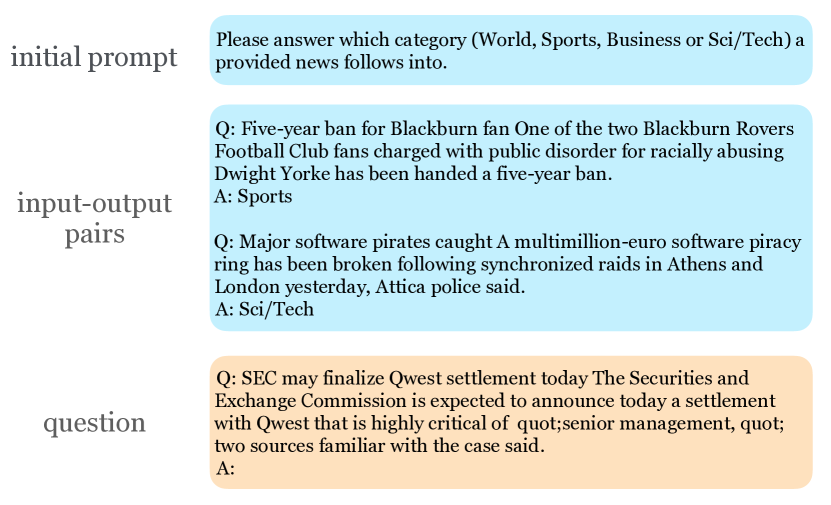
Figure 2. Prompt template for AGNews dataset.

Prompt Engineering. We design two-shot prompting templates for text-classification datasets to ensure models generate outputs in the desired format. For AGNews, we adopt the prompt template from FrugalGPT (Chen et al., 2023) but limit input-output examples to two, as shown in Figure 2. The blue text blocks contain the prompt and examples, while the orange block contains the target question. This structure is applied across all datasets. For other datasets in text classification, we randomly select two training records as input-output pairs. For datasets in entity matching, we follow the procedure outlined in (Peeters et al., 2025) and use a zero-shot prompt with two templates: domain-complex for DBLP-Scholar and Amazon-Google, and general-complex for the others.

(a) Overruling

(b) AGNews

(c) SciQ

(d) Hellaswag

(e) Banking77

Figure 3. Accuracy vs cost for text classification query.

6.2. Performance on Text Classification Query

The tested methods are evaluated in terms of accuracy scores against LLM usage costs. Figure 3 presents the results of the accuracy versus costs of the $3$ tested methods except for LLM-Blender on the five datasets. In particular, FrugalGPT encounters the out-of-memory issue on our machine (24GB GPU memory) on dataset Hellaswag, so its performance is not reported in Figure 3d. Moreover, FrugalGPT enforces budget constraints based on the expected training cost and does not respect the budget constraint strictly in a per-query manner, unlike ThriftLLM. For a fair comparison, we modify the budget constraint of FrugalGPT on testing queries to align with this per-query approach in our experiments. LLM-Blender utilizes all $12$ LLM candidates for response collection, subsequently aggregating the most prominent responses to formulate the final solution. Given that LLM-Blender is not budget-aware, it is not appropriate to compare it with budget-constrained methods across different budget scenarios. As such, we report the performance of LLM-Blender and compare it with ThriftLLM separately in Table 5.

Comparison with GreedyLLM and FrugalGPT. Figure 3 demonstrates the accuracy scores with the corresponding utilized cost of each method on the $5$ datasets for text classification queries. As shown, ThriftLLM consistently outperforms all other baseline models with either superior accuracy at the lowest costs or the highest accuracy with lower costs on all datasets. In particular, it achieves the highest accuracy on $4$ out of the $5$ tested datasets, except on Banking77. ThriftLLM may select several weaker models instead of stronger ones on Banking77. This selection discrepancy arises because the success probabilities of these weaker models are overestimated when queries are from a substantial number of distinct classes. Compared with GreedyLLM, ThriftLLM acquires comparable accuracy scores but consumes notably lower costs. This observation demonstrates the effectiveness of adaptive selection in ThriftLLM on cost saving without sacrificing the performance. On datasets AGNews, Hellaswag, and Banking77, where the accuracy scores do not approach $1$, ThriftLLM exhibits an ability to enhance accuracy further as costs increase. This indicates that ThriftLLM effectively harnesses the capabilities of the LLM ensemble and scales efficiently with increased budget allocation.

Overall, ThriftLLM demonstrates a steadily strong performance, outperforming both GreedyLLM and FrugalGPT. The analysis reveals a general trend where ThriftLLM provides higher accuracy at lower cost levels, indicating its efficiency in utilizing computational resources.

Table 5. Accuracy (%) of ThriftLLM and LLM-Blender.

Dataset	Overruling	AGNews	SciQ	Hellaswag	Banking77
ThriftLLM	95.60	86.45	99.25	89.94	73.82
LLM-Blender	89.35	83.02	90.06	53.18	52.08

Comparison with LLM-Blender. In Table 5, we compare the best accuracy scores of ThriftLLM across five different budget settings with the accuracy of LLM-Blender, which uses all model outputs as candidates for response selection. Despite this, it can be seen that on all datasets ThriftLLM clearly outperforms LLM-Blender by a significant margin. Distinct from the response aggregation mechanism in ThriftLLM, LLM-Blender relies on the GenFuser component, a generative model fine-tuned on the T5-like architecture, to generate the final outputs by fusing collected candidate responses with additional query interpretations, which, however, leads to suboptimal quality. These results reveal the superior performance of ThriftLLM over LLM-Blender in text classification even with smaller budgets.

(a) WDC Products

(b) Abt-Buy

(c) Walmart-Amazon

(d) Amazon-Google

(e) DBLP-Scholar

Figure 4. F1 score vs cost for entity matching query.

6.3. Performance on Entity Matching Query

Figure 4 displays the F1 scores against the utilized costs of the three tested models. RoBERTa and Ditto, both based on the BERT (Kenton and Toutanova, 2019) architecture, are fine-tuned tailored for each tested dataset. Consistent with the experiment settings in (Peeters et al., 2025), we incorporate their reported results for RoBERTa and Ditto to ensure comparability. However, note that the corresponding utilization costs are not disclosed in (Peeters et al., 2025). To address this gap, we estimate the average cost per query by leveraging the reported fine-tuning time and the corresponding AWS pricing for computation time, given that their experiments were conducted on a p3.8xlarge AWS EC2 machine with 4 V100 GPUs (1 GPU per run).

As shown in Figure 4 for entity matching queries, ThriftLLM persistently dominates the other two baselines, yielding higher F1 scores but incurring lower costs on the four e-commerce datasets and acquiring the highest F1-score on DBLP-Scholar. In particular, ThriftLLM boosts the F1 scores with a notable improvement of $3.51\%$, $4.39\%$, $5.84\%$, $6.42\%$, and $0.30\%$ on the $5$ datasets respectively. Meanwhile, the observed performance pattern, where F1 scores increase with increasing budgets, signifies the strength of ThriftLLM to maximize the efficiency of allocated budgets thereby enhancing overall performance. This observation demonstrates that ThriftLLM aggregates less expensive LLMs in an effective manner, yielding superior performance at reduced costs.

6.4. Ablation Study

Table 6. Accuracy (%) for various confidence intervals on AGNews.

$\alpha$	0	0.02	0.04	0.08	0.1
Acc. of $\mathcal{P}_{\textrm{low}}$	84.80	84.93	84.80	84.80	84.74
Acc. of $\mathcal{P}_{\textrm{up}}$	84.80	84.80	84.87	84.73	84.80

Confidence interval on approximation guarantees. Let $\alpha$ represent the length of the confidence interval in Section 4.4, i.e., $\alpha=p^{\top}_{l}-p^{\bot}_{l}$ for $l\in[L]$. Specifically, given the current estimated probability $\hat{p}_{l}$, we set $p^{\bot}_{l}=\hat{p}_{l}-\tfrac{\alpha}{2}$ and $p^{\top}_{l}=\min\{\hat{p}_{l}+\tfrac{\alpha}{2},1.0\}$. By feeding the resultant probability sets $\mathcal{P}_{low}=\{p^{\bot}_{1},p^{\bot}_{2},\cdots,p^{\bot}_{L}\}$ and $\mathcal{P}_{up}=\{p^{\top}_{1},p^{\top}_{2},\cdots,p^{\top}_{L}\}$ to ThriftLLM respectively, we record the accuracy scores of the selected LLMs.

We vary $\alpha=\{0,0.02,0.04,0.08,0.1\}$ and conduct this experiment on dataset AGNews with the budget $B=1\times 10^{-5}$. The results are reported in Table 6. The accuracy score of $84.80\%$ with $\alpha=0$ acts as the base case. Compared with this case, accuracy scores with $\alpha>0$ are either the same or approximate $84.80\%$ with slight variations incurred by the inherent randomness of accuracy estimation in model selection. This observation reveals that ThriftLLM is robust to the estimated success probabilities.

Table 7. Accuracy (%) of ThriftLLM v.s. single LLMs.

Dataset	Overruling	AGNews	SciQ	Hellaswag	Banking77
ThriftLLM	95.60	86.45	99.25	89.86	73.82
GPT-4o	94.68	86.71	99.17	93.29	75.05
Gemini-1.5 Pro	95.14	89.01	96.61	90.96	25.91
Phi-3-medium	95.14	84.21	98.50	88.73	59.84
Llama-3 70B	94.68	81.31	98.86	86.53	69.66
Mixtral-8x7B	94.90	79.34	96.29	N.A.	N.A.

Table 8. Accuracy (%) using various historical data on Overruling.

Budget	$20\%$	$40\%$	$60\%$	$80\%$	Original
$1.0\times 10^{-5}$	95.37	94.91	96.06	94.90	95.14
$5.0\times 10^{-5}$	95.37	95.37	95.60	95.13	95.37
$10.0\times 10^{-5}$	95.37	95.37	95.37	95.60	95.37
$50.0\times 10^{-5}$	95.60	95.37	95.37	95.13	95.37
$100.0\times 10^{-5}$	95.60	95.37	95.37	95.60	95.60

ThriftLLM vs Single LLM. To further validate the advantage of the LLM ensemble over an individual LLM, we compare the accuracy scores obtained by ThriftLLM with single models in Table 4 on the $5$ tested datasets for text classification queries. For a convincing comparison, we select the most powerful and most expensive LLMs provided by each company, including GPT-4o from OpenAI, Gemini-1.5 Pro from Google, Phi-3-medium from Microsoft, Llama-3 70B from Meta, and Mixtral-8x7B from Mistral AI. The results are summarized in Table 7. For clarity, we highlight the highest accuracy score in bold and underline the second-highest score for each dataset.

As displayed, ThriftLLM achieves the best on $2$ out of $5$ datasets and second best on one of the remaining datasets. On the other $3$ datasets, ThriftLLM either achieves or closely approaches the second-highest accuracy scores with negligible gaps. This evidence not only underscores the superior performance of ThriftLLM as an ensemble model across diverse topics but also suggests that individual powerful models do not consistently offer advantages across all domains.

(a) Accuracy

(b) Cost

Figure 5. Accuracy vs Cost on Overruling.

Adaptive selection. We have proved (see Proposition 6) that the subset of LLMs selected by ThriftLLM makes the same prediction as that selected by SurGreedyLLM, while utilizing lower budgets. To verify this point and quantify the saved costs, we evaluate ThriftLLM and SurGreedyLLM on dataset Overruling by following the budget $B$ setting. The results are displayed in Figure 5.

As shown in Figure 5a, ThriftLLM and SurGreedyLLM achieve exactly the same accuracy scores, consistent with our result in Proposition 6. Figure 5b presents the comparison between their cost proportions relative to the given budgets. It is worth noting that ThriftLLM achieves a saving of $\sim 10\%\mbox{-}40\%$ of the allowed budget compared to SurGreedyLLM. Furthermore, as the budget decreases, the cost savings achieved by ThriftLLM compared to SurGreedyLLM become more noticeable.

Sensitivity to size of historical data. In text classification, $80\%$ of the dataset is used as historical data for success probability estimation. To evaluate the sensitivity of ThriftLLM to the size of historical data, we select $\{20\%,40\%,60\%,80\%\}$ of the original historical data on Overruling respectively for probability estimation, and then evaluate the performance of ThriftLLM on test queries by varying the budget $B=\{1.0,5.0,10,50,100\}\times 10^{-5}$ (see Table 8). The performance of ThriftLLM is stable and robust relative to the proportion of available historical data. The stability is further enhanced with increased budget allocations. These results imply that ThriftLLM consistently performs well across a wide range of sizes of available historical data.

7. Conclusion

We investigate the problem of finding an LLM ensemble under budget constraints for optimal query performance, with a focus on classification queries. We formalize this problem as the Optimal Ensemble Selection problem. To solve this problem, we design a new aggregation scheme for combining individual LLM responses and devise a notion of prediction accuracy to measure the aggregation quality. We prove that prediction accuracy is non-decreasing and non-submodular. Despite this, we develop ThriftLLM, a surrogate greedy algorithm that offers an instance dependent approximation guarantee. We evaluate ThriftLLM on several real-world datasets on text classification and entity matching tasks. Our experiments show that it achieves state-of-the-art performance while utilizing a relatively small budget compared to the baselines tested. Extensions of ThriftLLM to regression and generation tasks are intriguing directions for future work.

Appendix A Appendix: Proofs

Proof of Lemma 1.

For part (i), note that as the success probabilities of models increase, it is trivial that the prediction accuracy is non-decreasing. We focus on part (ii) in what follows.

Consider a random query $q\in\mathcal{Q}$ with ground-truth class $C_{q}$, any LLM set $\mathcal{S}\subset\mathcal{L}$, and model $l\in\mathcal{L}\setminus\mathcal{S}$. Let $\mathcal{S}^{\prime}:=\mathcal{S}\cup\{l\}$. We prove that $\xi(\mathcal{S}^{\prime})\geq\xi(\mathcal{S})$. Part (ii) will follow from this.

Let $\Omega$ and $\Omega^{\prime}$ be the observation spaces of $\mathcal{S}$ and $\mathcal{S}^{\prime}$ on query class $\mathcal{Q}$, respectively. Let $\Omega_{T}$ (resp. $\Omega^{\prime}_{T}$) be the subspace containing observations with the correct prediction $C_{q}$ and $\Omega_{F}=\Omega\setminus\Omega_{T}$ (resp. $\Omega^{\prime}_{F}=\Omega^{\prime}\setminus\Omega^{\prime}_{T}$) be the remaining subspace with incorrect predictions for $\mathcal{S}$ (resp. $\mathcal{S}^{\prime}$). When invoking the additional LLM $l$ on $\mathcal{Q}$, the observation space $\Omega$ is converted into $\Omega^{\prime}$: each observation $\phi_{\mathcal{S}}\in\Omega$ is uniquely mapped to $K$ distinct observations $\phi_{\mathcal{S}^{\prime}}\in\Omega^{\prime}$ with $\phi_{\mathcal{S}^{\prime}}=\phi_{\mathcal{S}}\oplus R(l)$, where $K$ is the number of classes, $\oplus$ is the concatenation operation, and response $R(l)\in\{C_{1},C_{2},\cdots,C_{K}\}$. Note that $Pr[\phi_{{\mathcal{S}^{\prime}}}]=\sum_{R(l)\in\{C_{1},C_{2},\cdots,C_{K}\}}Pr[\phi_{\mathcal{S}}\oplus R(l)]$.

Consider the scenarios involving $\phi_{\mathcal{S}}$ and $\phi_{\mathcal{S}^{\prime}}$: (1) observation $\phi_{\mathcal{S}}\in\Omega_{F}$ generates observations $\phi_{\mathcal{S}^{\prime}}\in\Omega^{\prime}_{T}$, and (2) observation $\phi_{\mathcal{S}}\in\Omega_{T}$ generates observations $\phi_{\mathcal{S}^{\prime}}\in\Omega^{\prime}_{F}$. We prove the probability of scenario (1) is no smaller than the probability of scenario (2). Notice that the other two scenarios, where observations in $\Omega_{T}$ (resp. $\Omega_{F}$) generate those in $\Omega^{\prime}_{T}$ (resp. in $\Omega^{\prime}_{F}$), do not contribute to changes in the prediction accuracy between $\xi_{\mathcal{P}}(\mathcal{S})$ and $\xi_{\mathcal{P}}(\mathcal{S}^{\prime})$.

Let $\phi^{\prime}_{x}\in\Omega^{\prime}_{F}$ be an observation generated from $\phi_{x}\in\Omega_{T}$ corresponding to scenario (2). Suppose $R(l)=C_{k}$, so $\phi^{\prime}_{x}=\phi_{x}\oplus C_{k}$. Since $\phi_{x}\in\Omega_{T}$ and $\phi^{\prime}_{x}\in\Omega^{\prime}_{F}$, we know $H_{1}(\phi_{x})=h(C_{q}\mid\phi_{x})$ and $H_{1}(\phi^{\prime}_{x})=h(C_{k}\mid\phi^{\prime}_{x})$ where $C_{q}\neq C_{k}$. This fact implies that the ranking of belief values of the $K$ classes is altered after applying the additional model $l$. Therefore, we can infer the inequality

(10) $$H_{1}(\phi^{\prime}_{x})=h(C_{k}\mid\phi^{\prime}_{x})=h(C_{k}\mid\phi_{x})\tfrac{p_{l}(K-1)}{1-p_{l}}>h(C_{q}\mid\phi_{x}),$$

where $p_{l}$ is the success probability of model $l$.

We can derive an observation pair corresponding to scenario (1) from the observation pair above. To start with, observe the inherent symmetry of the observation space. To explain, for observation space $\Omega$, there exists an observation pair $(\phi,\phi^{\circ})$ in $\Omega$ such that an arbitrary model outputs $C_{q}$ in $\phi$ if and only if it outputs $C_{k}$ in $\phi^{\circ}$ and vice versa, and for models outputting a class outside $\{C_{q},C_{k}\}$, the two observations coincide. Denote by $\mathcal{S}(C_{i}\mid\phi)$ the set of models which predict the class $C_{i}$ as per the observation $\phi$. By virtue of the symmetry property, there exists an observation $\phi_{y}\in\Omega_{F}$ symmetric to $\phi_{x}$ from $\Omega_{T}$ such that $\mathcal{S}(C_{k}\mid\phi_{y})=\mathcal{S}(C_{q}\mid\phi_{x})$, $\mathcal{S}(C_{q}\mid\phi_{y})=\mathcal{S}(C_{k}\mid\phi_{x})$, and the remaining LLMs $\mathcal{S}_{r}=\mathcal{S}\setminus(\mathcal{S}(C_{q}\mid\phi_{x})\cup\mathcal{S}(C_{k}\mid\phi_{x}))$ make the same predictions in both $\phi_{x}$ and $\phi_{y}$. Therefore, it holds that $H_{1}(\phi_{y})=h(C_{k}\mid\phi_{y})$. In such a case, consider the case $R(l)=C_{q}$ and the corresponding $\phi^{\prime}_{y}=\phi_{y}\oplus C_{q}$. According to Equation (10), we have

(11) $$h(C_{q}\mid\phi_{y})\tfrac{p_{l}(K-1)}{1-p_{l}}=h(C_{k}\mid\phi_{x})\tfrac{p_{l}(K-1)}{1-p_{l}}>h(C_{q}\mid\phi_{x})=h(C_{k}\mid\phi_{y}).$$

As a result, $H_{1}(\phi^{\prime}_{y})=h(C_{q}\mid\phi^{\prime}_{y})=h(C_{q}\mid\phi_{y})\tfrac{p_{l}(K-1)}{1-p_{l}}$, i.e., $\phi^{\prime}_{y}\in\Omega^{\prime}_{T}$, and the observation pair $(\phi_{y},\phi\prime_{y})$ corresponds to scenario (1).

We now prove that the probability of scenario (1) is no smaller than that of scenario (2), i.e., accuracy gain from scenario (1) should be no less than the accuracy loss due to scenario (2). In particular, for $Pr[\phi^{\prime}_{y}]$, we have

$$Pr[\phi^{\prime}_{y}]= \prod_{l_{i}\in\mathcal{S}(C_{q}\mid\phi^{\prime}_{y})}p_{i}\prod_{l_{i}\in\mathcal{S}(C_{k}\mid\phi^{\prime}_{y})}\tfrac{1-p_{i}}{K-1}\prod_{l_{i}\in\mathcal{S}_{r}}\tfrac{1-p_{i}}{K-1}$$

$$= \prod_{l_{i}\in\mathcal{S}(C_{q}\mid\phi_{y})\cup\{l\}}p_{i}\prod_{l_{i}\in\mathcal{S}(C_{k}\mid\phi_{y})}\tfrac{1-p_{i}}{K-1}\prod_{l_{i}\in\mathcal{S}_{r}}\tfrac{1-p_{i}}{K-1}$$

$$= \prod_{l_{i}\in\mathcal{S}(C_{k}\mid\phi_{x})\cup\{\l\}}p_{i}\prod_{l_{i}\in\mathcal{S}(C_{q}\mid\phi_{x})}\tfrac{1-p_{i}}{K-1}\prod_{l_{i}\in\mathcal{S}_{r}}\tfrac{1-p_{i}}{K-1}$$

Similarly, for $Pr[\phi^{\prime}_{x}]$, we have

$$Pr[\phi^{\prime}_{x}]=\prod_{l_{i}\in\mathcal{S}(C_{q}\mid\phi_{x})}p_{i}\prod_{l_{i}\in\mathcal{S}(C_{k}\mid\phi_{x})\cup\{l\}}\tfrac{1-p_{i}}{K-1}\prod_{l_{i}\in\mathcal{S}_{r}}\tfrac{1-p_{i}}{K-1}.$$

When calculating the ratio of $\tfrac{Pr[\phi^{\prime}_{y}]}{Pr[\phi^{\prime}_{x}]}$, it holds that

$$\tfrac{Pr[\phi^{\prime}_{y}]}{Pr[\phi^{\prime}_{x}]}= \tfrac{\prod_{l_{i}\in\mathcal{S}(C_{k}\mid\phi_{x})\cup\{\l\}}p_{i}\prod_{l_{i}\in\mathcal{S}(C_{q}\mid\phi_{x})}\tfrac{1-p_{i}}{K-1}}{\prod_{l_{i}\in\mathcal{S}(C_{q}\mid\phi_{x})}p_{i}\prod_{l_{i}\in\mathcal{S}(C_{k}\mid\phi_{x})\cup\{l\}}\tfrac{1-p_{i}}{K-1}}$$

$$= \tfrac{\prod_{l_{i}\in\mathcal{S}(C_{k}\mid\phi_{x})\cup\{\l\}}p_{i}}{\prod_{l_{i}\in\mathcal{S}(C_{k}\mid\phi_{x})\cup\{l\}}\tfrac{1-p_{i}}{K-1}}\tfrac{\prod_{l_{i}\in\mathcal{S}(C_{q}\mid\phi_{x})}\tfrac{1-p_{i}}{K-1}}{\prod_{l_{i}\in\mathcal{S}(C_{q}\mid\phi_{x})}p_{i}}$$

$$= h(C_{k}\mid\phi_{x})\tfrac{p_{l}(K-1)}{1-p_{l}}\tfrac{1}{h(C_{q}\mid\phi_{x})}>1.$$

The last inequality follows from Equation (11). Let $\Omega^{\prime}_{x}$ and $\Omega^{\prime}_{y}$ be the set of such observations $\phi^{\prime}_{x}$ and $\phi^{\prime}_{y}$ respectively. Therefore $\xi(\mathcal{S}^{\prime})-\xi(\mathcal{S})=Pr[\Omega^{\prime}_{y}]-Pr[\Omega^{\prime}_{x}]$. As $Pr[\Omega^{\prime}_{y}]>Pr[\Omega^{\prime}_{x}]$, we have $\xi(\mathcal{S}^{\prime})>\xi(\mathcal{S})$. In particular, $\xi(\mathcal{S}^{\prime})=\xi(\mathcal{S})$ holds if both $\Omega^{\prime}_{x}$ and $\Omega^{\prime}_{y}$ are empty sets, which completes the proof. ∎

Proof of Lemma 2.

We construct a counterexample to demonstrate that the function $\xi(\mathcal{S})$ is not submodular. Consider sets $\mathcal{S}=\{l_{1}\}$, $\mathcal{T}=\{l_{1},l_{2}\}$, and a LLM $l_{3}$. W.l.o.g., we assume their success probabilities follow the partial ranking of $p_{1}>p_{2}$, $p_{1}>p_{3}$, and $\tfrac{p_{2}(K-1)}{1-p_{2}}\tfrac{p_{3}(K-1)}{1-p_{3}}>\tfrac{p_{1}(K-1)}{1-p_{1}}$, i.e., $\tfrac{p_{2}p_{3}(K-1)}{(1-p_{2})(1-p_{3})}>\tfrac{p_{1}}{1-p_{1}}$. As $\tfrac{p}{1-p}\in(0,\infty)$ for $p\in(0,1)$ and $\tfrac{p_{1}}{1-p_{1}}>\tfrac{p_{2}}{1-p_{2}}$ and $\tfrac{p_{1}}{1-p_{1}}>\tfrac{p_{3}}{1-p_{3}}$ hold simultaneously, such $p_{1},p_{2},p_{3}$ always exist when fixing $K$. If set function $\xi(\cdot)$ is submodular, it should satisfy

(12) $$\xi(\mathcal{S}\cup\{l_{3}\})-\xi(\mathcal{S})\geq\xi(\mathcal{T}\cup\{l_{3}\})-\xi(\mathcal{T}).$$

According to Proposition 3, we have $\xi(\mathcal{S})=\xi(\mathcal{S}\cup\{l_{3}\})=\xi(\mathbf{T})=p_{1}$. For $\xi(\mathcal{T}\cup\{l_{3}\})$, since $p_{1}>p_{2}$, $p_{1}>p_{3}$, and $\tfrac{p_{2}(K-1)}{1-p_{2}}\tfrac{p_{3}(K-1)}{1-p_{3}}>\tfrac{p_{1}(K-1)}{1-p_{1}}$ hold, the prediction accuracy $\xi(\mathcal{T}\cup\{l_{3}\})$ is the total probability of two cases: (i) $l_{1}$ makes the correct prediction while $\{l_{2},l_{3}\}$ fail to concur on the same incorrect prediction, and (ii) $l_{1}$ makes the incorrect prediction while $l_{2}$ and $l_{3}$ both predict correctly. Therefore, $\xi(\mathcal{T}\cup\{l_{3}\})$ is calculated as

$$\xi(\mathcal{T}\cup\{l_{3}\})=p_{1}-p_{1}(1-p_{2})\tfrac{1-p_{3}}{K-1}+(1-p_{1})p_{2}p_{3},$$

where the factor $p_{1}-p_{1}(1-p_{2})\tfrac{1-p_{3}}{K-1}$ is the probability of case (i) and the factor $(1-p_{1})p_{2}p_{3}$ is the probability of case (ii). As $\tfrac{p_{2}(K-1)}{1-p_{2}}\tfrac{p_{3}(K-1)}{1-p_{3}}>\tfrac{p_{1}(K-1)}{1-p_{1}}$, we have $(1-p_{1})p_{2}p_{3}-p_{1}(1-p_{2})\tfrac{1-p_{3}}{K-1}>0$. Therefore $\xi(\mathcal{T}\cup\{l_{3}\})>p_{1}=\xi(\mathcal{T})$. Hence Equation (12) does not hold, which completes the proof. ∎

Proof of Proposition 6.

Let $C_{\ast}$ be the class with $H_{1}(\phi_{\mathcal{S}})$, which implies $h(C_{\ast}\mid\phi_{\mathcal{S}})=\textstyle\prod_{l_{i}\in\mathcal{S}(C_{\ast})}\tfrac{p_{i}(K-1)}{1-p_{i}}$. The potential belief $F(\mathcal{T}^{\ast})=\prod_{l_{i}\in\mathcal{T}^{\ast}}\tfrac{p_{i}(K-1)}{1-p_{i}}$ is the highest possible belief that the remaining LLMs in $\mathcal{T}^{\ast}$ can contribute to any class. If $F(\mathcal{T}^{\ast})H_{2}(\phi_{\mathcal{S}})\leq H_{1}(\phi_{\mathcal{S}})$ holds, we have

$$F(\mathcal{T}^{\ast})H_{K}(\phi_{\mathcal{S}})\leq\cdots\leq F(\mathcal{T}^{\ast})H_{3}(\phi_{\mathcal{S}})\leq F(\mathcal{T}^{\ast})H_{2}(\phi_{\mathcal{S}})\leq H_{1}(\phi_{\mathcal{S}}).$$

This inequality implies that the remaining models in $\mathcal{T}^{\ast}$ are not able to contribute the belief to any class except $C_{\ast}$ so as to achieve a belief higher than $H_{1}(\phi_{\mathcal{S}})$. Therefore, Proposition 6 holds. ∎

Proof of Theorem 8.

By Lemma 7, the prediction accuracy $\xi(\mathcal{S})$ of each inspected $\mathcal{S}\subseteq\mathcal{L}$ is estimated within error $\tfrac{\epsilon p^{\ast}}{2}$ with at least $1-\frac{\delta}{L^{2}}$ probability. Let $\mathcal{S}^{\ast}$ be the set returned from SurGreedyLLM with $\theta$ Monte Carlo simulations of $\xi(\cdot)$. Therefore, for $\mathcal{S}^{\ast}=\arg\max\{p^{\ast},\tilde{\xi}(\mathcal{S}_{1}),\tilde{\xi}(\mathcal{S}_{2})\}$, it holds that $|\xi(\mathcal{S}^{\ast})-\tilde{\xi}(\mathcal{S}^{\ast})|\leq\tfrac{\epsilon p^{\ast}}{2}$ with high probability. Since the set function $\gamma(\cdot)$ can be exactly computed in linear time, $\max\{\gamma(\mathcal{S}_{2}),p^{\ast}\}\geq(1-\tfrac{1}{\sqrt{{\mathrm{e}}}})\gamma(\mathcal{S}^{\circ}_{\gamma})$ holds without involving estimation errors.

As a consequence, we have

$$\tfrac{\xi(\mathcal{S}^{\ast})}{\xi(\mathcal{S}^{\circ})}\geq\tfrac{\tilde{\xi}(\mathcal{S}^{\ast})-\epsilon p^{\ast}/2}{\xi(\mathcal{S}^{\circ})}\geq\tfrac{\max\{\xi(S_{1}),\ \xi(S_{2}),\ p^{\ast}\}-\epsilon p^{\ast}}{\gamma(\mathcal{S}^{\circ})}$$

$$\geq\tfrac{\max\{\xi(S_{1}),\ \xi(S_{2}),\ p^{\ast}\}-\epsilon p^{\ast}}{\gamma(\mathcal{S}^{\circ}_{\gamma})}=\tfrac{\max\{\xi(S_{1}),\ \xi(S_{2}),\ p^{\ast}\}-\epsilon p^{\ast}}{\max\{\gamma(\mathcal{S}_{2}),p^{\ast}\}}\tfrac{\max\{\gamma(\mathcal{S}_{2}),p^{\ast}\}}{\gamma(\mathcal{S}^{\circ}_{\gamma})}$$

$$\geq\tfrac{\max\{\xi(S_{1}),\ \xi(S_{2}),\ p^{\ast}\}-\epsilon p^{\ast}}{\max\{\gamma(\mathcal{S}_{2}),\ p^{\ast}\}}(1-\tfrac{1}{\sqrt{{\mathrm{e}}}})$$

$$\geq(\tfrac{\max\{\xi(S_{1}),\ \xi(S_{2}),\ p^{\ast}\}}{\max\{\gamma(\mathcal{S}_{2}),\ p^{\ast}\}}-\epsilon)(1-\tfrac{1}{\sqrt{{\mathrm{e}}}}).$$

Considering that at most $L^{2}$ possible subsets are checked in GreedyLLM, the failure probability is bounded by union bound $\frac{\delta}{L^{2}}\cdot L^{2}=\delta$. Therefore, it holds that

$$\Pr\left[\xi(\mathcal{S}^{\ast})\geq(\tfrac{\max\{\xi(S_{1}),\ \xi(S_{2}),\ p^{\ast}\}}{\max\{\gamma(\mathcal{S}_{2}),\ p^{\ast}\}}-\epsilon)(1-\tfrac{1}{\sqrt{{\mathrm{e}}}})\cdot\xi(\mathcal{S}^{\circ})\right]\geq 1-\delta,$$

which completes the proof. ∎

Proof of Theorem 9.

By taking $\mathcal{P}_{\textrm{low}}$, $\hat{\mathcal{P}}$, and $\mathcal{P}_{\textrm{up}}$ as inputs to ThriftLLM, let $\xi_{l}(\mathcal{S}^{\circ}_{l})$, $\xi(\mathcal{S}^{\circ})$, and $\xi_{u}(\mathcal{S}^{\circ}_{u})$ be the accuracy scores of the corresponding optimal sets respectively, and $\xi_{l}(\mathcal{S}^{\ast}_{l})$, $\xi(\mathcal{S}^{\ast})$, and $\xi_{u}(\mathcal{S}^{\ast}_{u})$ be the accuracy scores of the selected sets for $\mathcal{P}_{\textrm{low}}$, $\hat{\mathcal{P}}$, and $\mathcal{P}_{\textrm{up}}$ respectively. According to Theorem 8, we have

$$\Pr\left[\tfrac{\xi(\mathcal{S}^{\ast})}{\xi(\mathcal{S}^{\circ})}\geq(\tfrac{\max\{\xi(S_{1}),\ \xi(S_{2}),\ p^{\ast}\}}{\max\{\gamma(\mathcal{S}_{2}),\ p^{\ast}\}}-\epsilon)(1-\tfrac{1}{\sqrt{{\mathrm{e}}}})\right]\geq 1-\delta.$$

Similarly, for $\mathcal{P}_{\textrm{up}}$, we have

$$\Pr\left[\tfrac{\xi_{u}(\mathcal{S}^{\ast}_{u})}{\xi_{u}(\mathcal{S}^{\circ}_{u})}\geq(\tfrac{\max\{\xi_{u}(S_{u1}),\ \xi_{u}(S_{u2}),\ p^{\ast}_{u}\}}{\max\{\gamma_{u}(\mathcal{S}_{u2}),\ p^{\ast}_{u}\}}-\epsilon)(1-\tfrac{1}{\sqrt{{\mathrm{e}}}})\right]\geq 1-\delta,$$

where $\gamma_{u}(\cdot)$ is the surrogate set function, $S_{u1}$ and $S_{u2}$ are selected by SurGreedyLLM on $\mathcal{P}_{\textrm{up}}$, respectively. As $p^{\bot}_{l}\leq p_{l}\leq p^{\top}_{l}$ for $l\in[L]$ holds w.p. $\geq 1-\delta_{l}$, according to the non-decreasing property of $\xi(\cdot)$ (Lemma 1), we have $\xi(\mathcal{S}^{\circ})\leq\xi_{u}(\mathcal{S}^{\circ}_{u})$ and $\xi_{l}(\mathcal{S}^{\ast}_{l})\leq\xi(\mathcal{S}^{\ast})$. Therefore, we have

$$\tfrac{\xi(\mathcal{S}^{\ast})}{\xi(\mathcal{S}^{\circ})}\geq\tfrac{\xi_{l}(\mathcal{S}^{\ast}_{l})}{\xi_{u}(\mathcal{S}^{\circ}_{u})}\geq\tfrac{\xi_{l}(\mathcal{S}^{\ast}_{l})}{\xi_{u}(\mathcal{S}^{\ast}_{u})}(\tfrac{\max\{\xi_{u}(S_{u1}),\ \xi_{u}(S_{u2}),\ p^{\ast}_{u}\}}{\max\{\gamma_{u}(\mathcal{S}_{u2}),\ p^{\ast}_{u}\}}-\epsilon)(1-\tfrac{1}{\sqrt{{\mathrm{e}}}}).$$

Meanwhile, as proved in Theorem 8, there are at most $L^{2}$ possible subsets for accuracy estimation. Therefore, each model is involved in estimation at most $L^{2}$ times. Therefore, the resulting failure probability is at most $\delta+L^{2}\sum^{L}_{l=1}\delta_{l}$. Consequently, we have

$$\Pr\left[\tfrac{\xi(\mathcal{S}^{\ast})}{\xi(\mathcal{S}^{\circ})}\geq\tfrac{\xi_{l}(\mathcal{S}^{\ast}_{l})}{\xi_{u}(\mathcal{S}^{\ast}_{u})}(\tfrac{\max\{\xi_{u}(S_{u1}),\ \xi_{u}(S_{u2}),\ p^{\ast}_{u}\}}{\max\{\gamma_{u}(\mathcal{S}_{u2}),\ p^{\ast}_{u}\}}-\epsilon)(1-\tfrac{1}{\sqrt{{\mathrm{e}}}})\right]$$

$$\geq 1-(\delta+L^{2}\textstyle\sum^{L}_{l=1}\delta_{l}),$$

which completes the proof. ∎

Proof of Lemma 10.

Let $X_{1},X_{2},\cdots,X_{\Lambda_{l}}\in\{0,1\}$ be random variables such that $X_{i}=1$ if $p^{(i)\bot}_{l}\leq p_{l}\leq p^{(i)\top}_{l}$ holds where $[p^{(i)\bot}_{l},p^{(i)\top}_{l}]$ is the confidence interval obtained in the $i$-th repetition; otherwise $X_{i}=0$. Let $X=\tfrac{1}{\Lambda_{l}}\sum^{\Lambda_{l}}_{i=1}X_{i}$ be the average. Therefore, we have $\mathbb{E}[X]\geq 1-\delta_{l}$ as $X_{i}=1$ holds with at least $1-\delta_{l}$ probability. Let the value centered at the interval $[p^{(i)\bot}_{l},p^{(i)\top}_{l}]$ be the corresponding estimation. Among the total $\Lambda_{l}$ estimations after algorithm $\mathcal{A}$ is repeated $\Lambda_{l}$ times, let $[\bar{p}^{\bot}_{l},\bar{p}^{\top}_{l}]$ be the confidence interval whose estimation is the median value among obtained estimations. The true probability $p_{l}$ does not belong to $[\bar{p}^{\bot}_{l},\bar{p}^{\top}_{l}]$ if and only if at least half of the estimations fail, i.e., $X_{i}=0$. In this regard, we have

$$Pr[p_{l}\notin[\bar{p}^{\bot}_{l},\bar{p}^{\top}_{l}]]\leq\Pr[X\leq\tfrac{1}{2}]\leq\Pr[X\leq\mathbb{E}[X]-\tfrac{1-2\delta_{l}}{2}]$$

$$\leq \exp(-2\Lambda_{l}(\tfrac{1-2\delta_{l}}{2})^{2})=\exp(-\tfrac{\Lambda_{l}(1-2\delta_{l})^{2}}{2}),$$

where the second inequality is due to the fact that $\mathbb{E}[X]-\tfrac{1-2\delta_{l}}{2}\geq\tfrac{1}{2}$ as $\mathbb{E}[X]\geq 1-\delta_{l}$, and last inequality is due to Hoeffding’s inequality (Hoeffding, 1963). Thus Lemma 10 is proved. ∎

References

- (1)
- Anthropic (2024) Anthropic. 2024. Introducing the next generation of Claude. https://www.anthropic.com/news/claude-3-family Accessed on April 26, 2024.
- Bansal et al. (2024) Rachit Bansal, Bidisha Samanta, Siddharth Dalmia, Nitish Gupta, Sriram Ganapathy, Abhishek Bapna, Prateek Jain, and Partha Talukdar. 2024. LLM Augmented LLMs: Expanding Capabilities through Composition. In ICLR.
- Barlaug and Gulla (2021) Nils Barlaug and Jon Atle Gulla. 2021. Neural networks for entity matching: A survey. TKDD 15, 3 (2021), 1–37.
- Bian et al. (2017) Andrew An Bian, Joachim M. Buhmann, Andreas Krause, and Sebastian Tschiatschek. 2017. Guarantees for Greedy Maximization of Non-submodular Functions with Applications. In ICML, Vol. 70. 498–507.
- Boucheron et al. (2003) Stéphane Boucheron, Gábor Lugosi, and Olivier Bousquet. 2003. Concentration Inequalities. In Advanced Lectures on Machine Learning, Vol. 3176. 208–240.
- Buchbinder et al. (2012) Niv Buchbinder, Moran Feldman, Joseph Naor, and Roy Schwartz. 2012. A Tight Linear Time (1/2)-Approximation for Unconstrained Submodular Maximization. In FOCS. 649–658.
- Cappuzzo et al. (2020) Riccardo Cappuzzo, Paolo Papotti, and Saravanan Thirumuruganathan. 2020. Creating embeddings of heterogeneous relational datasets for data integration tasks. In SIGMOD. 1335–1349.
- Casanueva et al. (2020) Iñigo Casanueva, Tadas Temcinas, Daniela Gerz, Matthew Henderson, and Ivan Vulic. 2020. Efficient Intent Detection with Dual Sentence Encoders. In Proceedings of the 2nd Workshop on NLP for ConvAI - ACL 2020.
- Chen and Varoquaux (2024) Lihu Chen and Gaël Varoquaux. 2024. What is the Role of Small Models in the LLM Era: A Survey. arXiv preprint arXiv:2409.06857 (2024).
- Chen et al. (2023) Lingjiao Chen, Matei Zaharia, and James Zou. 2023. FrugalGPT: How to Use Large Language Models While Reducing Cost and Improving Performance. CoRR abs/2305.05176 (2023).
- Chen and Li (2024a) Wei Chen and Zhiyuan Li. 2024a. Octopus v2: On-device language model for super agent. CoRR abs/2404.01744 (2024).
- Chen and Li (2024b) Wei Chen and Zhiyuan Li. 2024b. Octopus v4: Graph of language models. CoRR abs/2404.19296 (2024).
- Dai et al. (2024) Xiangxiang Dai, Jin Li, Xutong Liu, Anqi Yu, and John C. S. Lui. 2024. Cost-Effective Online Multi-LLM Selection with Versatile Reward Models. CoRR abs/2405.16587 (2024).
- Ding et al. (2024) Dujian Ding, Ankur Mallick, Chi Wang, Robert Sim, Subhabrata Mukherjee, Victor Rühle, Laks V. S. Lakshmanan, and Ahmed Hassan Awadallah. 2024. Hybrid LLM: Cost-Efficient and Quality-Aware Query Routing. In ICLR.
- Ebraheem et al. (2018) Muhammad Ebraheem, Saravanan Thirumuruganathan, Shafiq Joty, Mourad Ouzzani, and Nan Tang. 2018. Distributed Representations of Tuples for Entity Resolution. VLDB 11, 11 (2018), 1454–1467.
- Fan et al. (2024) Ju Fan, Zihui Gu, Songyue Zhang, Yuxin Zhang, Zui Chen, Lei Cao, Guoliang Li, Samuel Madden, Xiaoyong Du, and Nan Tang. 2024. Combining Small Language Models and Large Language Models for Zero-Shot NL2SQL. VLDB 17, 11 (2024), 2750–2763.
- Fu et al. (2024) Xue-Yong Fu, Md. Tahmid Rahman Laskar, Elena Khasanova, Cheng Chen, and Shashi Bhushan TN. 2024. Tiny Titans: Can Smaller Large Language Models Punch Above Their Weight in the Real World for Meeting Summarization?. In NAACL. 387–394.
- Gan and Tao (2015) Junhao Gan and Yufei Tao. 2015. DBSCAN Revisited: Mis-Claim, Un-Fixability, and Approximation. In SIGMOD. 519–530.
- Gao et al. (2024) Dawei Gao, Haibin Wang, Yaliang Li, Xiuyu Sun, Yichen Qian, Bolin Ding, and Jingren Zhou. 2024. Text-to-SQL Empowered by Large Language Models: A Benchmark Evaluation. VLDB 17, 5 (2024), 1132–1145.
- Gemini Team et al. (2023) Rohan Anil Gemini Team, Sebastian Borgeaud, Yonghui Wu, Jean-Baptiste Alayrac, Jiahui Yu, Radu Soricut, Johan Schalkwyk, Andrew M. Dai, and Anja Hauth et al. 2023. Gemini: A Family of Highly Capable Multimodal Models. CoRR abs/2312.11805 (2023).
- Getoor and Machanavajjhala (2012) Lise Getoor and Ashwin Machanavajjhala. 2012. Entity resolution: theory, practice & open challenges. VLDB 5, 12 (2012), 2018–2019.
- help.openai.com (2024) help.openai.com. 2024. How much does GPT-4 cost? Retrieved Oct 17, 2024 from https://help.openai.com/en/articles/7127956-how-much-does-gpt-4-cost
- Hillier et al. (2024) Dylan Hillier, Leon Guertler, Cheston Tan, Palaash Agrawal, Chen Ruirui, and Bobby Cheng. 2024. Super Tiny Language Models. CoRR abs/2405.14159 (2024).
- Hoeffding (1963) Wassily Hoeffding. 1963. Probability Inequalities for Sums of Bounded Random Variables. J. Amer. Statist. Assoc. (1963), 13–30.
- Huang et al. (2020) Keke Huang, Jing Tang, Xiaokui Xiao, Aixin Sun, and Andrew Lim. 2020. Efficient Approximation Algorithms for Adaptive Target Profit Maximization. In ICDE. 649–660.
- Jiang et al. (2023) Dongfu Jiang, Xiang Ren, and Bill Yuchen Lin. 2023. LLM-Blender: Ensembling Large Language Models with Pairwise Ranking and Generative Fusion. In ACL. 14165–14178.
- Kenton and Toutanova (2019) Jacob Devlin Ming-Wei Chang Kenton and Lee Kristina Toutanova. 2019. Bert: Pre-training of deep bidirectional transformers for language understanding. In NAACL, Vol. 1.
- Khuller et al. (1999) Samir Khuller, Anna Moss, and Joseph Naor. 1999. The Budgeted Maximum Coverage Problem. Inf. Process. Lett. 70, 1 (1999), 39–45.
- Konda et al. (2016) Pradap Konda, Sanjib Das, Paul Suganthan G. C., AnHai Doan, Adel Ardalan, Jeffrey R. Ballard, Han Li, Fatemah Panahi, Haojun Zhang, Jeff Naughton, Shishir Prasad, Ganesh Krishnan, Rohit Deep, and Vijay Raghavendra. 2016. Magellan: toward building entity matching management systems. VLDB 9, 12 (2016), 1197––1208.
- Lei et al. (2023) Deren Lei, Yaxi Li, Mengya Hu, Mingyu Wang, Vincent Yun, Emily Ching, and Eslam Kamal. 2023. Chain of Natural Language Inference for Reducing Large Language Model Ungrounded Hallucinations. CoRR abs/2310.03951 (2023).
- Li et al. (2020) Yuliang Li, Jinfeng Li, Yoshihiko Suhara, AnHai Doan, and Wang-Chiew Tan. 2020. Deep entity matching with pre-trained language models. VLDB 14, 1 (2020), 50–60.
- Liu et al. (2019) Yinhan Liu, Myle Ott, Naman Goyal, Jingfei Du, Mandar Joshi, Danqi Chen, Omer Levy, Mike Lewis, Luke Zettlemoyer, and Veselin Stoyanov. 2019. RoBERTa: A Robustly Optimized BERT Pretraining Approach. arXiv preprint arXiv:1907.11692 (2019).
- livechatai.com (2024) livechatai.com. 2024. Gemini Pro API Pricing Calculator. Retrieved Oct 17, 2024 from https://livechatai.com/gemini-pro-api-pricing-calculator
- Martello and Toth (1987) Silvano Martello and Paolo Toth. 1987. Algorithms for knapsack problems. North-Holland Mathematics Studies 132 (1987), 213–257.
- Mudgal et al. (2018) Sidharth Mudgal, Han Li, Theodoros Rekatsinas, AnHai Doan, Youngchoon Park, Ganesh Krishnan, Rohit Deep, Esteban Arcaute, and Vijay Raghavendra. 2018. Deep learning for entity matching: A design space exploration. In SIGMOD. 19–34.
- OpenAI (2023) OpenAI. 2023. GPT-4 Technical Report. CoRR abs/2303.08774 (2023).
- O’Reilly-Morgan et al. (2025) Diarmuid O’Reilly-Morgan, Elias Tragos, Erika Duriakova, Honghui Du, Neil Hurley, and Aonghus Lawlor. 2025. Entity Matching with Large Language Models as Weak and Strong Labellers. In New Trends in Database and Information Systems. 58–67.
- Parciak et al. (2024) Marcel Parciak, Brecht Vandevoort, Frank Neven, Liesbet M. Peeters, and Stijn Vansummeren. 2024. Schema Matching with Large Language Models: an Experimental Study. VLDB 2024 Workshop: Tabular Data Analysis Workshop (TaDA) (2024).
- Peeters et al. (2025) Ralph Peeters, Aaron Steiner, and Christian Bizer. 2025. Entity Matching using Large Language Models. In EDBT. 529–541.
- Shekhar et al. (2024) Shivanshu Shekhar, Tanishq Dubey, Koyel Mukherjee, Apoorv Saxena, Atharv Tyagi, and Nishanth Kotla. 2024. Towards Optimizing the Costs of LLM Usage. CoRR abs/2402.01742 (2024).
- Shi and Lai (2024) Yishuo Shi and Xiaoyan Lai. 2024. Approximation algorithm of maximizing non-monotone non-submodular functions under knapsack constraint. Theor. Comput. Sci. 990 (2024), 114409.
- Su et al. (2019) Dan Su, Yan Xu, Genta Indra Winata, Peng Xu, Hyeondey Kim, Zihan Liu, and Pascale Fung. 2019. Generalizing Question Answering System with Pre-trained Language Model Fine-tuning. In EMNLP. 203–211.
- Sun et al. (2023) Xiaofei Sun, Xiaoya Li, Jiwei Li, Fei Wu, Shangwei Guo, Tianwei Zhang, and Guoyin Wang. 2023. Text Classification via Large Language Models. In EMNLP. 8990–9005.
- Sun et al. (2024) Yushi Sun, Xin Hao, Kai Sun, Yifan Xu, Xiao Yang, Xin Luna Dong, Nan Tang, and Lei Chen. 2024. Are Large Language Models a Good Replacement of Taxonomies? VLDB 17, 11 (2024), 2919–2932.
- Tang et al. (2024) Yehui Tang, Kai Han, Fangcheng Liu, Yunsheng Ni, Yuchuan Tian, Zheyuan Bai, Yi-Qi Hu, Sichao Liu, Shangling Jui, and Yunhe Wang. 2024. Rethinking Optimization and Architecture for Tiny Language Models. In ICML.
- Tang et al. (2014) Youze Tang, Xiaokui Xiao, and Yanchen Shi. 2014. Influence maximization: near-optimal time complexity meets practical efficiency. In SIGMOD. 75–86.
- Trummer (2024) Immanuel Trummer. 2024. Generating Succinct Descriptions of Database Schemata for Cost-Efficient Prompting of Large Language Models. VLDB 17, 11 (2024), 3511–3523.
- Wang et al. (2024) Mengzhao Wang, Haotian Wu, Xiangyu Ke, Yunjun Gao, Xiaoliang Xu, and Lu Chen. 2024. An Interactive Multi-modal Query Answering System with Retrieval-Augmented Large Language Models. VLDB 17, 12 (2024), 4333–4336.
- Welbl et al. (2017) Johannes Welbl, Nelson F. Liu, and Matt Gardner. 2017. Crowdsourcing Multiple Choice Science Questions. In Workshop on Noisy User-generated Text, NUT@EMNLP. 94–106.
- Xia et al. (2024) Yu Xia, Fang Kong, Tong Yu, Liya Guo, Ryan A. Rossi, Sungchul Kim, and Shuai Li. 2024. Which LLM to Play? Convergence-Aware Online Model Selection with Time-Increasing Bandits. In WWW. 4059–4070.
- Yao et al. (2022) Dezhong Yao, Yuhong Gu, Gao Cong, Hai Jin, and Xinqiao Lv. 2022. Entity resolution with hierarchical graph attention networks. In SIGMOD. 429–442.
- Zellers et al. (2019) Rowan Zellers, Ari Holtzman, Yonatan Bisk, Ali Farhadi, and Yejin Choi. 2019. HellaSwag: Can a Machine Really Finish Your Sentence?. In ACL. 4791–4800.
- Zhang et al. (2024b) Chao Zhang, Yuren Mao, Yijiang Fan, Yu Mi, Yunjun Gao, Lu Chen, Dongfang Lou, and Jinshu Lin. 2024b. FinSQL: Model-Agnostic LLMs-based Text-to-SQL Framework for Financial Analysis. In SIGMOD. 93–105.
- Zhang et al. (2024a) Tianyi Zhang, Faisal Ladhak, Esin Durmus, Percy Liang, Kathleen R. McKeown, and Tatsunori B. Hashimoto. 2024a. Benchmarking Large Language Models for News Summarization. ACL 12 (2024), 39–57.
- Zhang et al. (2015) Xiang Zhang, Junbo Jake Zhao, and Yann LeCun. 2015. Character-level Convolutional Networks for Text Classification. In NIPS. 649–657.
- Zhao and He (2019) Chen Zhao and Yeye He. 2019. Auto-em: End-to-end fuzzy entity-matching using pre-trained deep models and transfer learning. In WWW. 2413–2424.
- Zheng et al. (2021) Lucia Zheng, Neel Guha, Brandon R. Anderson, Peter Henderson, and Daniel E. Ho. 2021. When does pretraining help?: assessing self-supervised learning for law and the CaseHOLD dataset of 53, 000+ legal holdings. In ICAIL. 159–168.
- Zhu et al. (2024) Jun-Peng Zhu, Peng Cai, Kai Xu, Li Li, Yishen Sun, Shuai Zhou, Haihuang Su, Liu Tang, and Qi Liu. 2024. AutoTQA: Towards Autonomous Tabular Question Answering through Multi-Agent Large Language Models. VLDB 17, 12 (2024), 3920–3933.