Distributed network of smartphone sensors: a new tool for scientific field measurements

Abstract

Smartphones are widespread objects that have been used as physics sensors for the general public thanks to their availability, high connectivity and built-in sensors. Here, we present the use of a fleet of smartphones to create a distributed network of time-synchronized sensors. We first evaluate the sensors quality in the laboratory and then describe the network configuration that allows the remote control of an entire fleet. Finally, we present two test cases that use the smartphone fleet for physical field measurements. By this study, we show that this approach paves the way for large-scale field scientific studies.

I Introduction

By November 2024, mobile subscriptions have reached 8.4 billion, including 7.14 billion for smartphones Jonsson (2024). The widespread use of smartphones has also made them a key tool for educational and scientific research purposes thanks to their accessibility to the general public Gao and Wu (2016); Raju et al. (2024) and to their built-in micro-electro-mechanical system (MEMS) sensors. A typical MEMS is a highly integrated, silicon-based sensor system fabricated using semiconductor processes Maluf (2002). Its low cost, compact size, lightweight design, and low power consumption make a MEMS ideal for integration into smartphones, drones, tablets, and wearable devices Daponte et al. (2013), enabling applications such as step counting and orientation tracking Bao and Intille (2004); Naqvib et al. (2012); Davidson and Piché (2016), gaming Höpfner et al. (2013); Kołakowska, Szwoch, and Szwoch (2020), and navigation Li et al. (2015); Mostafa et al. (2019), etc.

In the context of physics education, following the COVID-19 pandemic, smartphones have gained popularity as flexible tools for providing innovative teaching methodologies, particularly at the university level Bobroff, Bouquet, and Delabre (2020); Bouquet et al. (2020); O’Brien (2021). Numerous examples on conducting tabletop physics experiments can be given such as measuring the speed of sound with the embedded microphone Kasper, Vogt, and Strohmeyer (2015); estimating the earth’s rotation using the accelerometer Vandermarlière (2021); and light polarization analyses using ambient light sensor Monteiro et al. (2017). Comprehensive reviews of examples can be found in Organtini Organtini et al. (2021) and in Kuhn $\&$ Vogt  Kuhn and Vogt (2022).

The versatility of smartphone MEMS sensors has also drawn significant attention from researchers across various scientific domains. The high connectivity and ubiquity of smartphones enable large-scale, real-time data collection through a geographically distributed network of interconnected devices. For public health research, investigations on the data collection and analysis of energy expenditure from smartphone users Pande et al. (2013) have shown that smartphone-embedded IMU (Inertial Measurement Unit) sensors such as accelerometers and gyroscopes, can accurately monitor the user’s physical activities, thus enhance the precision of individual health assessments. In a review by Lee et al. Lee, Suh, and Choi (2018) on smartphone applications in geoscience research, the authors highlight the growing use of smartphones in tasks traditionally carried out with specialized tools, such as geological mapping, seismic activity detection, and natural hazard assessment.

However, field measurements in large-scale physical applications require multi-point data collection with sensors spatially distributed over a wide area while remaining synchronized in time. Examples of such applications include predicting solar magnetic storms and assessing their impact on Earth’s magnetosphere Odenwald (2022), as well as performing modal analysis of civil engineering structures Guéguen et al. (2020), where a large number of data points are crucial for reconstructing higher-order spatial modes Cunha and Caetano (2006); Rainieri and Fabbrocino (2014). Distributed sensor measurements in seismology using smartphones have been introduced via real-time data collections for earthquake detection using the application MyShake Kong, Allen, and Schreier (2016). It allows accurate localization of the earthquake’s epicenter and detects seismic waves propagation in real time, contributing to early warning systems Reilly et al. (2013); Kong, Allen, and Schreier (2016). These applications do not rely on sophisticated, high-cost sensors but rather utilize frugal, cost-effective sensor networks, such as smartphone-based MEMS sensors fleets on a large scale, often in regions geographically inaccessible through traditional methods.

Several mobile applications (PhyPhox, FizziQ) Staacks et al. (2018); Bilgin, Molina Ascanio, and Minoli (2022) have been developed for individual users to facilitate sensor communication and to display data in real-time. However, there is a notable lack of a technical way to control multiple smartphones by a single user. In contrast to single smartphone measurement that can be performed with manual interactions, distributed measurements require an automated process involving remote communication for data sampling and collection, time synchronization between smartphones, and parallel task planification. Another key challenge lies in the optimization of human-machine interaction (HMI) for a single user to control a fleet smartphone.

In this study, we present a methodology to perform simultaneous multi-sensor measurements using a fleet of identical smartphones. The article is structured as follows: we first review the measurement accuracy of a single smartphone using several test set up. We characterize in particular the ambient noise amplitude and spectrum of a single smartphone placed in a still environment. We then perform accelerometer and gyroscope sensor calibration and we determine their locations by conducting sensor measurements on a turntable platform Mau et al. (2016) with error quantification provided. This retro-engineering approach allows to precisely determine the sensor locations that are otherwise proprietary for most commercial products. Next, we developed an automated remote communication and control protocol for data recording across the smartphone fleet, achieving time synchronization with a typical error of 50 $\mu$s. Finally, we introduced a custom Android-based application, Gobannos Zhang, Eddi, and Perrard (2024), which integrates parametric memory allocation for data storage, remote communication, and fleet time synchronization. At the end of the article, we provide two examples illustrating the implementation of fleet measurements, demonstrating the feasibility of reliable data collection using a large fleet of smartphones.

II Smartphones as a multi-sensor fleet

To create a fleet of autonomous, multi-physics sensors, we selected the Redmi 10A smartphone, balancing cost (104 € each) and the quality of the embedded IMU sensors (accelerometer, gyroscope and magnetometer). The fleet is composed of 66 smartphones, numbered from 0 to 65. We use concomitantly the accelerometer, gyroscope, magnetometer and GPS sensors. To access and utilize the smartphone sensors, we initially employed the Phyphox application Staacks et al. (2018), developed at the University of Aachen. Phyphox offers an intuitive interface for acquiring data from individual sensors or from multiple sensors simultaneously, along with a standard URL communication protocol to retrieve data from the smartphone. We configured a module in Phyphox to simultaneously collect accelerometer, gyroscope, magnetometer, and GPS data at their respective maximum sampling frequencies. In a second step, we develop an Android application, named Gobannos, better adapted to parallelized, continuous and time synchronized acquisitions without physical intervention on the phones. This section is organized as follow. Section A presents the mechanical tests performed on the smartphone sensors. Section B details the architecture we develop to control a smartphone fleet from a single computer.

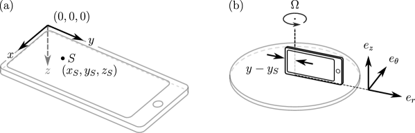
Figure 1: (a) Sketch of the smartphone coordinate system ($0,x,y,z$) with the origin located on the top-right up corner of the phone’s bounding box. The accelerometer sensor is located at point $S$. (b) Sketch of the turning-table setup used for the sensor tests.

II.1 Sensor tests

The coordinate system of the smartphone sensors is shown in Fig. 1(a), according to the direction of the acceleration of gravity measured along the three main axes (Fig. 1(a)). Note that the $(x,y,z)$ coordinate frame of the phone forms an indirect base. The smartphones are equipped with built-in IMU sensors model ICM-42670-P fabricated by TDK InvenSense invenSense (2021).

We first characterize the noise amplitude of the smartphone sensors using recordings in a quiescent environment. We then mount a smartphone on a rotating table to identify the exact location $S$ of the accelerometer. We eventually use the same experimental set up to calibrate the gyroscope sensor.

II.1.1 Noise amplitude and spectrum

We first perform tests on the noise level of the smartphone sensors. We perform five-minute recordings in a quiescent environment with the accelerometer, the gyroscope and the magnetometer. The typical sampling frequency of the accelerometer is 400 Hz, with variations from a smartphone to another of about 1%. Note that for each smartphone, the sampling frequency is stable over time. A typical value of the sampling frequency is $fs=403.96\pm 0.06$ Hz (smartphone # 30). The typical acceleration error is $\sigma_{a}$ = 0.02 m s^-2 in the direction perpendicular to gravity and $\sigma_{a}$ = 0.07 m s^-2 along the direction of gravity. We notice that the gyroscope was sold by the constructor as a 400 Hz sampling frequency sensor, however in practice, it only operates at 50 Hz. Typical error is $\sigma_{g}=0.004$ rad/s.

We interpolate the signal on a regular grid in time at a sampling frequency close to their maximum sensor sampling frequency (resp. 400 Hz for $a$ and 50 Hz for $g$ and $m$), and compute the temporal power spectrum $\hat{a}_{i}$, $\hat{g}_{i}$ and $\hat{m}_{i}$ of the acceleration, angular velocity, and magnetic field components (resp. $a_{i}$, $g_{i}$ and $m_{i}$). The power spectrum of one component for each sensor type (resp. $a_{z}$, $g_{y}$ and $m_{x}$) is shown in Fig. 2(a), (b) and (c) as a function of the frequency. The noise acceleration spectrum is flat in the entire range of tested frequency $f\in[0.1,200]$ Hz. We observe residual vibrations peaks at large frequencies. However, they may be specific to the contact between the phone and the ground, and the amplitude and locations of the peaks may not be reproducible. The noise spectrum of the gyroscope data is colored (see Fig. 2(b)) with a maximum of sensitivity at 1 Hz. The magnetometer exhibits a typical error $\sigma_{m}=1~\mu$T about one hundred time smaller than the Earth magnetic field. The associated noise spectrum is also colored, with a steeper slope than the gyroscope, and secondary lobes above 5 Hz.

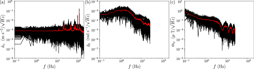
Figure 2: Noise spectrum of accelerometer (a), gyroscope (b) and magnetometer (c) computed on a noise recordings of 17 minutes (red curve). Each black line corresponds to a single phone recording. Note that the sampling frequency is around 400 Hz for the accelerometer, while it is only 50 Hz for both gyroscope and magnetometer.

About 15% of the smartphones showed a parasitic beat signal on the gyroscope sensors, and were relegated to the last number of the series. The first 50 smartphones sensors all show comparable quality of their sensors. Note that the smartphones do not share continuous serial numbers, and do not necessarily come from the same manufactured series.

II.1.2 Accelerometer sensor location

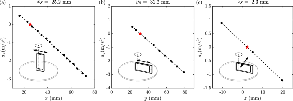
Figure 3: Determination of the accelerometer sensor location along the three main smartphone axis. a), b) and c) Measurements of respectively $a_{x}$, $a_{y}$, $a_{z}$ as a function of the sliding position $x$ (resp. $y$, $z$), for a rotation axis $Z$ aligned with $y$ (resp. $x$, $x$). In the three cases we observe a linear relationship, which intersects zero at the sensor position $x_{S}$ (resp. $y_{S}$, $z_{S}$) denoted by the black stars.

We mount a smartphone on a table, rotating around a vertical axis ($Z$) at an angular frequency $\Omega$ (Fig. 1(b)). We conduct three series of experiments, with the smartphone placed with its axis $x$ (resp. $y$ and $z$) aligned with the vertical axis $Z$. We vary the smartphone position with respect to the rotation axis by sliding it radially (sketches of Fig. 3(a) and (b)) or tangentially (sketch Fig. 3(c)). We then record the acceleration and gyroscope signals for 60s. From a force balance in the rotating frame of reference, we expect the radial acceleration (along $e_{r}$) to be $a_{x}$ = $r\Omega^{2}$ (resp. $a_{y}$ and $a_{z}$). The acceleration $a_{x}$ vanishes when the sensor is located on the rotation axis. Note that origin of space is taken at the upper top right corner of the phone, as sketched on Fig. 1(a). Fig. 3(a,b,c) show respectively the radial accelerations $a_{x}$, $a_{y}$ and $a_{z}$ for the smartphone rotating respectively along $y$, $x$ and $x$ axes at the angular frequency $\Omega=7.7$ rad/s as a function of the smartphone locations. We indeed find a linear relationship with $r$, and we extract the position of the sensor along the three axes by interpolating the curves in $a$=0, represented by the black stars. We found $x_{S}=25.2\pm 0.1$ mm, $y_{S}=31.2\pm 0.1$ mm and $z_{S}=2.3\pm 0.1$ mm. The slope of the linear relation, $a_{x}$ = $r\Omega^{2}$ can be used to check the accuracy of the accelerometer, knowing the rotation rate $\Omega$. We found an excellent agreement (less than 1 % error) in all three direction of orientations.

Figure 4: Calibration of accelerometer and gyroscope. The measurement depends on the axis of rotation. When the smartphone rotate around the position of the gyroscope, it actually measures the angular velocity within 1% of error. When the smartphone rotates around an off-centered axis, the measured values depend on the distance $r$ to the axis of rotation. This discrepancy originates from hardware limitations. (a) 3-axis acceleration signals recorded for a rotating phone. (b) 3-axis gyroscope signals recorder in the same rotating configuration. (c) Total gyroscopic signal $g=\sqrt{g_{x}^{2}+g_{y}^{2}}$ in this rotating configuration. (d) Measured angular velocity along $y$ from $g_{x}$ signal, as a function of the position of the smartphone with respect to the rotation axis, compared to the expected value. The imposed angular speed $\Omega$ is color-coded. e) Measurement along $g_{y}$, corresponding to a rotation around $x$ that does not physically occur. This corresponds to a systematic error, which increases linearly with $r$, and increases with rotation speed. From these measurements, we infer that the minimal error is reached when the smartphone rotates around the position of the gyroscope, we find $r_{g}=31.3\pm 1$mm, different from the accelerometer location. f) Percentage of error $g_{y}/(\Omega r)$ as a function of the angular velocity $\Omega$, in cm^-1.

II.1.3 Accelerometer $\&$ gyroscope calibration

We now test the gyroscope accuracy using the same set up, with the accelerometer data as the reference. We rotate the phone along the $x$ axis at an angular frequency $\Omega=7.7$ rad/s, varying the position of the phone with respect to the rotation axis (sketch of Fig. 3(b)). Fig. 4(a) shows the average acceleration as a function of the relative sensor position $y-y_{S}$ to the rotation axis. The three colors corresponds to the components $a_{x}$, $a_{y}$ and $a_{z}$ of the acceleration. We recover that the sensor measures the acceleration of gravity along the $y$ axis for all sliding positions, the centrifugal force along $x$, and the $z$ component is identically zero. Fig. 4(b) shows the average angular velocity components $g_{x},g_{y}$ and $g_{z}$ measured simultaneously by the gyroscope, as a function of the relative smartphone position $y-y_{S}$. The main rotation is indeed found along $y$, and the value agrees quantitatively with less than 0.5% of error when the accelerometer sensor is on the rotation axis ($y=y_{s}$). However, we also measures a linear variation of $g_{x}$ as a function of $y-y_{S}$ and a small (quadratic) decrease of $g_{y}$. These measurements do not correspond to a true phone rotation as evidenced by the accelerometer signals, but rather to a limitation of the gyroscope sensor. In this specific case of a known rotation axis, the systematic error can be compensated, by noticing that $g=\sqrt{g_{x}^{2}+g_{y}^{2}}$ is conserved for all tested smartphone positions $y-y_{S}$ (Fig. 4(c)), and correspond to the imposed angular frequency $\Omega$. The same behaviour is observed for all three directions of rotation. This discrepancy originates from the limitation of the measurement technique implemented in the gyroscope sensor. In practice, the gyroscope is a vibrating structure gyroscope (VSG) which is based on the Coriolis effect applied on a vibrating mass. As a consequence, in a non Galilean frame of reference, the gyroscope measures a combination of inertial acceleration and Coriolis force, and the sensor reading deviates from the true angular frequency, both in magnitude and in direction. To further test the gyroscope sensor limitations, we perform additional measurements with increasing rotation rate, at four different phone locations $y-y_{S}$ for a rotation around the $x$ axis of the phone. Fig. 4(d) shows the main angular velocity component $g_{x}$ as a function of $y-y_{S}$, for different rotation rates (color coded). These measurements confirm that for small $\Omega$ (typically $\Omega$< 5 rad/s), we recover $g_{x}\sim\Omega$. For larger rotation rate, we observe a significant discrepancy, which depends on the smartphone location. In particular for $|y-y_{S}|$ = 50mm the error grows to 10% at $\Omega=10$ rad/s. The systematic error is best evidenced by the signals of $g_{y}$ (Fig. 4(e)), which should be identically zero. For all rotation speeds, the systematic error is linear with the distance $r$ between the sensor and the axis of rotation, and the slope increases with $\Omega$. From these measurements, we infer that the gyroscope sensor is located at the position $y_{g}=31.3\pm 1$ mm along the $y$ axis, very close to the accelerometer sensor. Eventually, we extract the slope $\alpha_{g}$ of the error $g_{y}=\alpha_{g}(r-r_{g})$, and we compute a relative error, $\Delta g=\alpha_{g}/\Omega$, which is measured in $\%/cm$, as it is an error proportional to $r$. The error is represented in Fig. 4(f) as a function of $\Omega$. For a period of 1s corresponding to $\Omega=2\pi$ rad/s, we found 4% of error per centimeter .

We conclude that in practice, the gyroscope is reliable only to measure pure rotational motions around the gyroscope sensor, and cannot be used in general in combination with the accelerometer to decompose arbitrary superposition of translational and rotational motions. However, in some limit cases, in particular when the center of rotation is known, we expect the gyroscope to be reliable. One may refer to Fig. 4(f) to evaluate the systematic error as a function of both the angular frequency and the distance $r$ between the sensor and the axis of rotation.

II.2 Smartphone fleet remote control

II.2.1 Remote control of a single smartphone

Numerous smartphone applications exist to record the phone sensor data. We first use the application Phyphox Staacks et al. (2018) developed at the university of Aachen, which provides a user-friendly interface to acquire data from several sensors in parallel. Phyphox provides in particular a standard url communication protocol to send instructions (START, STOP, CLEAR) from a distant host. The sensor data can also be downloaded remotely using the Phyphox URL protocol (SAVE). We parametrize Phyphox with an experimental module that acquires simultaneously the accelerometer, gyroscope, magnetometer and GPS data at their respective maximum sampling frequencies. As described below in this section, we managed to use Phyphox simultaneously on a fleet of 60 smartphones to run acquisitions and gather data remotely. However, we have faced several limitations inherent to the Phyphox design. First, Phyphox does not continuously save the sensor data on the smartphone internal storage, such that the recordings accumulate in a buffer memory, limiting the duration of continuous recordings. Second, Phyphox requires an initial physical access to the phone to activate the distant access. Third, no time synchronisation protocol with a distant host is implemented. To circumvent these three limitations, we developed an Android smartphone application called Gobannos (github link). This application allows to remotely access the smartphone sensors, continuously save the sensor data on the smartphone memory, and to synchronize the phone clock with a remote computer with a better accuracy.

II.2.2 Network configuration & remote control of the fleet

To operate the fleet remotely, we connect all smartphones to the same Wi-Fi network. We use a Wi-Fi broadcast system that supports at least 70 parallel connections. A laptop connected to this local network, namely the controller, is used as a DHCP server for Wi-Fi broadcast system. This controller is also used to send remote instructions to the smartphone fleet. The DHCP server attributes to each smartphone a static IP address 192.168.X.1YY, where YY is the smartphone identification number, and X is the local network identifier. The correspondence between the MAC address and the IP is saved in a text file, and used to write the configuration file of the DHCP server. We notice that the network parameters also need to be set to static IP address within each smartphone to avoid Wi-Fi disconnections when there is no internet connexion on the local Wi-Fi network. Eventually, we can identify each smartphone with its static IP address.

All the smartphones run on the same version of the Android operating system. We use Android Debug Bridge (ADB) to communicate command line instructions to the smartphones from the controller. However, ADB protocol has to be authorized on the phone, and the procedure depend on the smartphone type and the constructor. We first unlock the developer mode manually on each smartphone. To authorize ADB USB connections, Xiaomi required a Mi account associated with a personal SIM card and an email address. Each series of 3 smartphones required a different combination of SIM card and email address to be unlocked, but up to 6 smartphones could be unlocked for each email address using two different SIM cards. We then used 22 different SIM cards and 11 generic email addresses to unlock the 66 smartphones. Once connected to a Mi account, we allow the ADB USB connections, and the SIM card can then be removed. This procedure is a priori specific to Redmi, as other constructors do not necessarily require personal information to authorize ADB USB connections.

Prior to each day of experiment, each smartphone was connected to the controller using an USB cable, and an ADB connection was set automatically using a script adb_usb.sh. The script uses a second table to map the ADB USB unique smartphone identifier to the right IP address. The ADB links are stable for at least a day, as long as the smartphone is connected continuously to the Wi-Fi. The individual ADB links between the controller and the smartphones are used to start Phyphox remotely, check the phone state (battery level, temperature, activity), and exchange files between the controller and the smartphones. Once the Phyphox communication protocol is enabled, we use url instructions to start, stop, and save the data remotely.

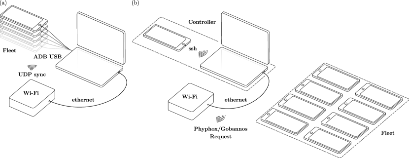
Figure 5: Conceptual sketch for (a) fleet remote control installation protocol and (b) fleet field deployment protocol.

II.2.3 Time synchronisation

The time synchronisation of a distributed network such as a smartphone fleet is challenging. For synchronizing clocks in a distributed network, the Network Time protocol (NTP) was introduced and normalised in 1985 and is used to synchronise computer clocks over internet Mills (1991). For better performance, the Precision Time Protocol (PTP) Eidson, Fischer, and White (2002) was later introduced. Both protocols use information exchange between a server and a client, to estimate the time delay between their internal clocks. The delay introduced by the communication time between the two machines is deduced, by assuming that the communication time is symmetric, and does not depend on time. The typical precision of a NTP protocol on a local network is of the order of 1ms, while a PTP protocol can go down to $\mu$s precision in optimal conditions.

To test the clock synchronisation using standard protocol, we implemented manually a network time protocol (NTP) and performed $10^{5}$ time requests between a server and 3 test smartphones using ADB time requests. Due to standard delays in Wi-Fi communication protocol, the typical duration of a time request is 100 milliseconds. Overall, the error of the NTP was found to be of few ms for a optimal Wi-Fi communication (direct line, less than 3 meter distance), but rises up to 100ms for larger Wi-Fi distance. In optimal conditions, we used these time requests to estimate the properties of the phone clock. We found that the typical delay between two phones is of the order of 1 second, a much larger delay than the precision of the GPS clock. However, the time difference between two phone clocks is stable over time: we identify less than 1ms of time drift between two smartphone clocks over 10 hours. A time synchronisation every day was then found to be sufficient.

In practice, a mechanical time synchronisation gives a typical error of few ms between the smartphone clocks, and was found to be sufficient for most applications.

Thanks to Gobannos, we later used UDP commands to synchronize the phone clocks, and we achieve a much better time synchronisation, with a typical error of 50$\mu$s after averaging on 100 time requests performed on each phone.

II.2.4 Pyphone application

To facilitate the remote control of the smartphone fleet, we developed a Python application called pyphone available on github.com Zhang, Eddi, and Perrard (2024), which implements the functionnalities described above. It includes in particular the DHCP server configuration, the creation of ADB links, the start of Phyphox remotely, the control of Phyphox or Gobannos acquisitions through the url protocol (run, stop clear and save) and the check of the phone states (Temperature, battery level). To optimize time delays in the execution of a command on multiple phones, we use asynchronous Python functions. We also use multi-threading to allocate a thread to each task type. Several tasks can then be run in parallel on a subpart of the smartphone fleet. Pyphone uses a graphical interface based on PyQt5 with buttons and tabs to organize the functions in themes, and run the commands on the selected phones.

III Applications

Here we present two applications of the smartphone fleet as time synchronized IMU sensors. The first section is devoted to the oscillation of a smartphone chain immersed in a turbulent flow. Each phone is then used both as the object of interest and the measuring device. The second section is devoted to the use of smartphones as local wave buoys, when placed on sea ice covering water. Recording the acceleration, angular velocity and earth magnetic field, we manage to measure the wave amplitude and wave spectrum at different locations.

III.1 Pendulum chain in turbulence

The environmental artist Ned Kahn’s artworks “Kinetic Façade” are building facades covered by thousands of aluminium pendulum plates that oscillate harmoniously in the wind, creating regular patterns of ripples that resemble a fluttering flag Shelley and Zhang (2011) or sea waves Drazin (2002); Perrard et al. (2019). To gain in-depth understanding of such phenomena, recent experimental investigations by Zhang and Perrard Zhang and Perrard (2024) were conducted on oscillation measurement of a 1 meter chain of pendulum plates confronting a turbulent flow by camera imaging. They have evidenced wave-like advective patterns of pendulums oscillations, similar to Ned Kahn’s artworks. By spectral analyses in spatiotemporal Fourier space of the pendulum oscillations, it has been shown that these moving patterns could emerge in turbulent flow as a result of two distinct mechanisms. One can be described as a resonant response of each pendulum near the pendulum’s natural frequency of oscillation and the other one attributes to the direct response of the pendulums to the turbulent fluctuations. The maximum response is reached at the intersection between the two dispersion relations.

To upscale the observable pendulum plate dynamics to a larger flow dimension comparable to that of a real facade, we used smartphones as rigid plate pendulums to measure spatiotemporal pressure fluctuations. We constructed a ten-meter-long chain of 60 uniformly spaced smartphones, each one hinged to a common rod along its top edge, allowing free oscillation around the $x$-axis. The built-in sensors, including accelerometers and gyroscopes, enable the determination of the instantaneous tilt angle of each smartphone. This setup provides highly temporally resolved measurements of oscillations and is space-efficient, especially where imaging techniques using cameras reach their limits.

Measurements of the chain oscillation in the wind flow were conducted in the large low speed S6 wind tunnel at Institut Aérotechnique Saint-Cyr-l’École l’Ecole (2025). The chain of smartphones was placed in the symmetry line of the facility’s test section, as shown in Fig. 6 (a). The free-stream wind speed $U$ is varied in the range 2-10 m/s, allowing an interaction of a fully established turbulent flow with the smartphone chain. The instantaneous and time-averaged statistics of the wind flow speed were measured independently via calibrated hotwire probes and dynamic pressure sensors.

Fig. 6 shows the spatiotemporal chart of the tangential accelerations $a_{z}$ measured by the chain of smartphones. From left to right of the chart, we observe wavy patterns propagating across the chain with an approximately constant phase speed. We also observe interference patterns with reflected waves that propagate upstream. Two ten-second instantaneous time signals of tangential and radial accelerations are shown in Fig. 6 (inset). We see that the smartphone orientation is periodic at well defined frequencies through both signals. The radial acceleration (black curve) is seen to oscillate at a frequency twofold larger than that of the tangential acceleration (red curve). This frequency doubling originates from the contribution of the term $\ell_{S}\dot{\theta}^{2}$ where $\ell_{S}$ is the $y$ distance from the accelerometer to the rod and $\theta(t)$ the time dependent orientation of the smartphone.

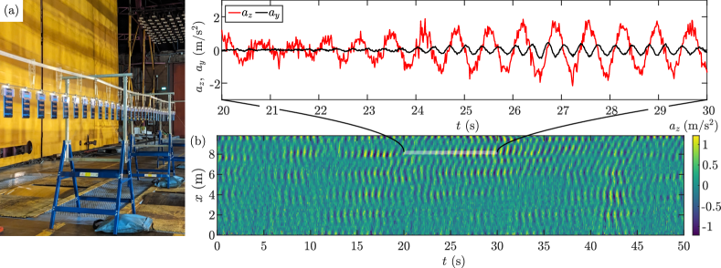
Figure 6: a) Image of the wind tunnel measurement setup. The chain of smartphones is placed in the symmetry plane of the measuring section, in suspension with metal trestles. b) Spatiotemporal chart of the tangential acceleration $a_{z}$ of the chain of telephones, for a wind speed $U=9.3$ m/s. Inset: temporal signal of the tangential $a_{z}$ and radial acceleration $a_{y}$ of the smartphone $\#50$ located at around $x=8$ m. Both the signal duration and smartphone position are indicated by the white dashed line.

III.2 Wave buoys

The smartphone fleet can also be used as a network of autonomous IMU systems in outdoor conditions. We perform a proof of concept during a field campaign on wave sea ice interaction in Rimouski, Québec, Canada, during February 2024, where the smartphones were deployed as local wave buoys to record the motion of ice induced by gravity waves.

As a proof of concept, we deployed smartphones as local wave buoys during a field campaign on wave–sea ice interaction, conducted in February 2024 near Rimouski, Québec, Canada. Smartphones can aptly be used to record the motion of the ice induced by gravity waves, as an array of smartphones can provide spatial and temporal information on wave propagation and attenuation. Custom ABS cases were 3D-printed to shield phones from the environmental condition, ensuring their temperature remains within working range.

On 23 February, we noticed wave activity sufficient to break the sea ice cover (thickness of 16 cm) in Mercier Cove, in the estuary of the Saint Lawrence river. We placed ten phones close to the forming ice edge, on a straight line, aligned with the direction of wave propagation, regularly spaced 10 meters apart. We recorded GPS coordinates, as well as acceleration, gyroscope and magnetometer signals. The recordings overlapped in time for about thirty minutes, and we only present the exploitation of vertical accelerations in this section, as a proxy for wave height. We show a top-view of the cropped situation, photographed by a drone, in Fig. 7(a).

The phone-recorded positions proved to be accurate, within about 5 m, to positions recorded with a hand-held GPS. Unfortunately, due to hardware limitation, from the moment phones where laid on the ice, the phone-recorded positions do not vary in time, which prevents us from extracting more precise positions through averaging. The precision of the location during the transport of the phones from their initialization location to their recording location is 12 cm/s.

Two of these phones were doubled with wave buoys, themselves equipped with geolocation and accelerometers. One of these buoys failed to provide usable data. After the time-synchronization of the phones signals, we set their time origin by finding the lag maximizing the cross-correlation between the acceleration signals of the phone (#T19) and the buoy (#B1) situated at the same location. We show the excellent correlation between the signals in Fig. 7(b).

In Fig. 7(c), we show the time evolution of the vertical acceleration as recorded by phones at increasing distance from the ice edge. Qualitatively, we confirm the synchronization of the signals by observing individual wave packets moving in space. The attenuation of the wave amplitude, due to the ice cover, is evident.

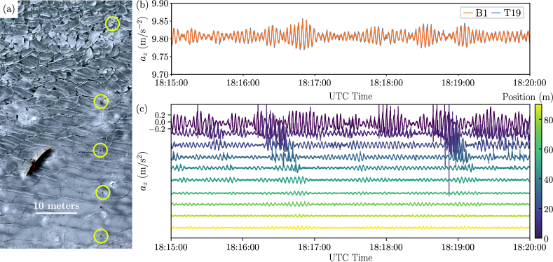
Figure 7: Experimental situation and temporal signals. (a) Top-view photographs of the experimental situation. The ice edge is at the top, and the ice becomes more continuous when moving away from it. Orange boxes (as seen next to the second phone, and between the fourth and fifth phones, counted from the top of the image) are wave buoys. Recording smartphones are highlighted with circles. (b) Comparison between vertical accelerations as measured by a phone and a wave buoy. The mean of the buoy signal as been adjusted to that of the phone to better visualize the agreement; the instrument bias is 0.035 m/s². (c) Temporal signals of ten smartphones placed 10 m apart, as described in the text. The distance is measured from the phone closest to the ice edge.

IV Conclusion

Smartphones are increasingly recognized for their potential in both scientific measurements and educational applications, owing to their integrated sensors and widespread accessibility. However, protocols for the deployment of smartphone fleets for distributed, real-time measurements remain underdeveloped. In this study, we conducted instrumental recordings with 66 smartphones using the embedded MEMS sensors. We first evaluated the sensors sensitivity and accuracy of a single smartphone and precisely determined the sensor locations. Based on existing protocols for single smartphones, we introduced the architectural development of Pyphone and Gobannos, a software framework designed for smartphone-based multi-physics instrumentation. To further test the robustness of our implementation, we provide two concrete examples of its application: large-scale physical measurements of turbulent fluctuations using smartphones as pendulums, and wave–ice floe interactions using smartphones as wave buoys. Altogether, our work paves the way for eco-friendly and low-cost solutions for large-scale scientific studies.