On cusps of caustics by reflection in two dimensional projective Finsler metrics

1 Motivation and previous results

In the posthumously published “Lectures on Dynamics”, Jacobi claimed that the conjugate locus of a non-umbilic point of a triaxial ellipsoid has exactly four cusps. This is known as the Last Geometric Statement of Jacobi. The conjugate locus of a point is the envelope of the geodesics that emanate from this point. These geodesics have the second, third, etc., envelopes; they are also called the first, second, etc., caustics.

The Last Geometric Statement of Jacobi was proved relatively recently [14]. Conjecturally, each next caustic also has exactly four cusps, see [18]. One also has a theorem, attributed to C. Carathéodory by W. Blaschke in his differential geometry textbook: The conjugate locus of a generic point on a convex surface has at least four cusps. See [20] for a recent proof.

One may consider a billiard version of this problem: instead of a closed surface, take a billiard table in the Euclidean plane bounded by an oval (smooth strictly convex closed curve), and instead of the pencils of geodesics, consider the pencil of billiard trajectories starting at a point inside the billiard table. After $n$ reflections off the boundary, one obtains a 1-parameter family of lines, and their envelope is the $n$th caustic by reflection. One may use the language of geometrical optics: the point is a source of light and the boundary curve is an ideal mirror.

This billiard problem was studied in two recent papers [7, 8]. We proved that for every oval, every $n\geq 1$, and a generic source of light the $n$th caustic by reflection has at least four cusps. We provided some evidence toward the conjecture that this number is exactly four for all $n$ if the billiard table is elliptic and proved this conjecture in the case when the boundary curve is a circle, see Figure 1. The context for these results is the famous 4-vertex theorem and its numerous variations and generalizations; see, e.g., [5].

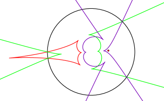
Figure 1: First three caustics by reflection in a circle.

In this note we extend this four cusps result to Finsler billiards in the special case of a projective Finsler metric, a (not necessarily symmetric) Finsler metric whose geodesics are straight lines.

2 Finsler metrics and Finsler billiards

From the point of view of geometrical optics, Finsler geometry describes the propagation of light in an inhomogeneous anisotropic medium $M$: the velocity of light depends on the point and the direction.

As usual, one has two descriptions of this process, the Lagrangian and the Hamiltonian ones. From the Lagrangian perspective, Finsler metric is defined by a field of indicatrices $I_{x}\subset T_{x}M$, the unit sphere subbundle of the tangent bundle of $M$. These indicatrices are unit level hypersurfaces of the Lagrangian function on $TM$ that defines the metric. The indicatrices are smooth and strictly convex hypersurfaces but, in general, not necessarily origin-symmetric.

The dual Hamiltonian description provides a field of figuratrices $J_{x}\subset T^{*}_{x}M$, the unit cosphere subbundle of the cotangent bundle of $M$. The indicatrices and figuratrices are related by the Legendre transform $D:I_{x}\to J_{x}$ (the polar duality):

$$I_{x}\ni v\mapsto w\in J_{x}\ \ {\rm if}\ \ {\rm Ker}\ w=T_{v}I_{x}\ \ {\rm and}\ \ w(v)=1.$$

A Finsler geodesic is a curve that extremizes the Finsler length (or optical path length) between its endpoints. The Finsler geodesic flow is defined similarly to the Riemannian case: the foot point of a Finsler unit tangent vector moves with the unit speed along the Finsler geodesic that it defines, and the vector remains unit and tangent to this geodesic.

We refer to any of the numerous textbooks on Finsler geometry or to the surveys [2, 10].

Finsler billiard reflection was defined in [13] similarly to the usual, Riemannian one, by a variational principle. Let $M$ be a Finsler manifold with boundary $S$, a billiard table, let $a$ and $b$ be two points in $M$ and $x$ be a boundary point. One says that the Finsler geodesic ray $ax$ reflects to the ray $xb$ if $x$ is a critical point of the Finsler distance function $F(x)={\rm dist}(ax)+{\rm dist}(xb)$. Note that, in general, the reflection is not reversible: it is not necessarily true that $bx$ reflects to $xa$.

Finsler billiard reflection can be described geometrically. This description is especially nice in dimension 2, which is the subject of this note. We continue to refer to [13].

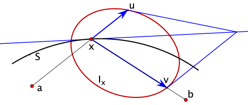
Figure 2: Finsler billiard reflection.

Consider Figure 2. The red oval is the indicatrix at the reflection point $x\in S$, and $u$ and $v$ are the incoming and outgoing unit velocity vectors. The reflection law states that the tangent lines to the indicatrix at points $u$ and $v$ and the tangent line to the boundary $S$ at point $x$ are concurrent (this includes the case when the three lines are parallel).

In the Euclidean case, the indicatrix is a circle, and this reflection law becomes the familiar “the angle of incidence equals the angle of reflection”.

A popular example of a Finsler billiards is a Minkowski billiard. In Minkowski geometry the indicatrices are parallel translation copies of each other and the geodesics are straight lines. A Minkowski billiard is defined by two ovals, the indicatrix and the billiard table. These billiards were studied in connection with the Viterbo conjecture in symplectic topology and its relation with the Mahler conjecture in convex geometry, see [6].

Concerning Minkowski billiards, also see [16].

Consider another example: the indicatrix is a focus-centered (Kepler) ellipse, see Figure 3. A theorem of elementary geometry states that $\angle AOC=\angle BOC$, see [4], Theorem 1.4 (this is known as “Le second théorème de Poncelet”, see the Wikipedia page “Théorème de Poncelet”).

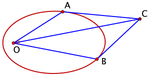
Figure 3: The indicatrix is a Kepler ellipse.

This result implies that the respective Finsler billiard reflection satisfies the same law of equal angles as the usual, Euclidean, one. This applies to another popular billiard model, the magnetic billiards. We follow the discussion in [19].

A magnetic field exerts a force on a moving charge that is perpendicular to the direction of motion and is proportional to the speed (Lorentz force). In particular, the speed of the charge remains constant.

A magnetic field in the plane is a given by a differential 2-form $B(x_{1},x_{2})dx_{1}\wedge dx_{2}$, where the function $B$ is the strength of the magnetic field. Choose a differential 1-form $\alpha$ such that $d\alpha=-B(x_{1},x_{2})dx_{1}\wedge dx_{2}$. The Lagrangian for the motion of a charge in this magnetic field is

$$L(x,v)=\frac{1}{2}|v|^{2}+\alpha(x)(v)$$

(the 1-form $\alpha$ is not unique, but the freedom of its choice does not affect the dynamics).

Following the Maupertuis principle, one replaces the Lagrangian by a homogeneous of degree one Lagrangian

$$L(x,v)=|v|+\alpha(x)(v)$$ (1)

whose extremals are the trajectories of the charge moving with the unit speed. In particular, if the magnetic field is constant,

$$L(x,v)=|v|+\frac{1}{2R}\det(v,x),$$

and the trajectories are counterclockwise oriented circles of (Larmor) radius $R$.

We assume that the magnetic field is sufficiently weak, so that $L(x,v)>0$ for $v\neq 0$ in the domain under consideration. More precisely, we assume that $|\alpha(x)|<1$ for all $x$.

Lemma 2.1

Let $L(x,v)$ be as in (1). Then, for every $x$, the indicatrix $L(x,v)=1$ is a focus-centered ellipse.

Proof.

The equation of a focus-centered axes-aligned ellipse in the $(v_{1},v_{2})$-plane is

$$\frac{(v_{1}+c)^{2}}{a^{2}}+\frac{v_{2}^{2}}{b^{2}}=1\ \ {\rm with}\ \ a^{2}=b^{2}+c^{2}.$$ (2)

We need to show that the equation $L(x,v)=1$ has this form.

Rotating the $v$-plane if needed, we may assume that $\alpha(x)(v)=tv_{1}$ with $|t|<1$. Then

$$\sqrt{v_{1}^{2}+v_{2}^{2}}+tv_{1}=1,$$

which is rewritten as

$$(1-t^{2})^{2}\left(v_{1}+\frac{t}{1-t^{2}}\right)^{2}+(1-t^{2})v_{2}^{2}=1.$$

Therefore, setting

$$a=\frac{1}{1-t^{2}},\ b=\frac{1}{\sqrt{1-t^{2}}},\ c=\frac{t}{1-t^{2}}$$

yields the desired equation (2). $\Box$

Thus the indicatrices of the magnetic Finsler metric are Kepler ellipses.

Magnetic billiards model the the motion of a charge in a a magnetic field with specular reflection off the boundary of the domain, so that the angle of incidence equals the angle of reflection, see Figure 4. Due to the “second theorem of Poncelet”, Figure 3, and Lemma 2.1, magnetic billiards are a particular case of Finsler billiards whose metric is defined by the Lagrangian (1).

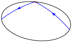
Figure 4: Magnetic billiard: the angle of incidence equals the angle of reflection.

We cannot help mentioning a multidimensional generalization of these results due to Akopyan and Karasev [3].

Theorem 1

Let $K$ be a smooth convex body in ${\mathbb{R}}^{n}$ containing the origin, and let $K_{1}$ be its convex image under a projective transformation that preserves, with orientation, every line passing through the origin. Then the Minkowski billiard reflection law in the space with the norm $K$ is the same as in the space with the norm $K_{1}$.

Such maps are given by the formula

$$x\mapsto\frac{tx}{1+\ell(x)},\ t>0,$$

where $\ell$ is a linear function. They send the origin-centered spheres to the focus-centered ellipsoids, in particular, origin-centered circles to Kepler ellipses.

Let us finish this section by adressing the symplectic properties of Finsler billiards. This properties do not play a major role in the present note, so we will be brief.

Assume that the space of oriented non-parameterized Finsler geodesics of $M$ is a smooth manifold. The Finsler billiard reflection defines a transformation of this space, the billiard ball map. This space of geodesics carries a symplectic structure constructed as follows.

Identify tangent and cotangent vectors via the Legendre transform. The cotangent bundle $T^{*}M$ has a canonical symplectic structure, and its restriction to the unit cosphere bundle has a 1-dimensional kernel at every point. The integral curves of this field of directions, the characteristics, are identified with the oriented non-parameterized Finsler geodesics of $M$. As a result, the space of characteristics carries a symplectic structure obtained from that in $T^{*}M$ by restriction to the unit cosphere bundle and factoring out the kernel. This construction is familiar in the Riemannian case, but it extends without change to the Finsler one.

A fundamental feature of Finsler billiards is that the billiard ball map preserves the symplectic structure of the space of oriented non-parameterized geodesics. It is important that this invariant symplectic form does not depend on the shape of the billiard table, it is determined by the ambient Finsler metric only. We refer to [13] for details.

3 Projective Finsler metric in two dimensions

In this section, we mostly follow the exposition in [1]. See [9, 15] for more details.

Hilbert’s fourth problem asks to construct and study the geometries in which the straight line segment is the shortest connection between two points. We interpret this problem (in dimension two, which is our concern in this note) as asking to describe Finsler metrics in convex subsets of the plane whose geodesics are straight segments. Such metrics are called projective.

The first examples are provided by Riemannian metrics of constant curvature, the Euclidean, spherical, and hyperbolic ones. The Euclidean case needs no explanation.

Consider a round sphere and project it from the center to a plane. This central projection takes great circles to straight lines, and it defines a projective metric in the plane that has a constant positive curvature.

A similar construction works for the hyperbolic plane presented by a hyperboloid of two sheets in Minkowski space: the central projection takes one sheet of the hyperboloid to the open unit disc, sending geodesics to straight lines. This yields the projective (Beltrami-Caley-Klein) model of the hyperbolic plane.

According to a Beltrami theorem, a projective Riemannian metric is a metric of constant curvature, so the above examples exhaust the Riemannian cases.

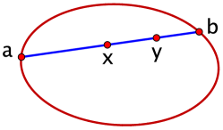
Figure 5: Hilbert’s and Funk’s metrics.

A Minkowski metric is an example of a projective Finsler metric. The projective model of the hyperbolic plane generalizes to Hilbert’s and to Funk’s metrics in a convex domain in the projective plane, see Figure 5, given by the formulas

$$d_{H}(x,y)=\frac{1}{2}\ln\left(\frac{|y-a||x-b|}{|y-b||x-a|}\right),\ \ d_{F}(x,y)=\ln\left(\frac{|x-b|}{|y-b|}\right)$$

(Hilbert’s metric is symmetric, while Funk’s metric is not). See [11] for a study of Funk billiards.

Let us introduce coordinates in the space ${\mathcal{L}}$ of oriented lines in ${\mathbb{R}}^{2}$. Choose an origin $O$. An oriented line is determined by its direction $\alpha\in S^{1}$ and its signed distance $p\in{\mathbb{R}}$ from the origin, see Figure 6. Thus ${\mathcal{L}}$ is an infinite cylinder.

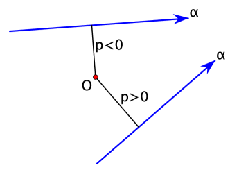
Figure 6: Coordinates in the space of oriented lines.

The symplectic structure on ${\mathcal{L}}$, invariant under the billiard ball transformation and described at the end of Section 2, is given by the 2-form $dp\wedge d\alpha$. Up to a factor, this is the unique area form on the space of lines that is invariant under isometries of the plane. We denote by $dA$ the respective area element.

We briefly describe a construction of symmetric projective Finsler metrics due to H. Buseman.

Recall the Cauchy-Crofton formula. Let ${\gamma}\subset{\mathbb{R}}^{2}$ be a piecewise smooth curve. Define a piecewise constant function on ${\mathcal{L}}$ to be the number of intersection points of a line with the curve. Then

$${\rm length}({\gamma})=\frac{1}{4}\int_{\ell\in\mathcal{L}}\#(\ell\cap{\gamma})\ dA.$$

Let $f:{\mathcal{L}}\to{\mathbb{R}}$ be a positive smooth function. Replace the area element $dA$ with $fdA$; then an analog of the Cauchy-Crofton formula defines a symmetric projective Finsler metric in the plane. We refer to [2] for more information.

4 The four cusps theorem

We finally turn to the main result of this note.

Let $U$ be an open plane domain with a projective (not necessarily symmetric) Finsler metric, and let ${\gamma}\subset U$ be an oval, the boundary of a Finsler billiard table. Let $O$ be a point inside ${\gamma}$ (the source of light). Consider the 1-parameter family of billiard trajectories, starting at $O$ and undergoing $n$ Finsler billiard reflections.

Theorem 2

For every $n\geq 1$, the envelope of this 1-parameter family of lines in ${\mathbb{RP}}^{2}$ (the $n$th caustic by reflection) has at least four cusps.

We need to comment on this formulation. Taken literally, it assumes that the $n$th caustic by reflection is a piecewise smooth curve whose smooth arcs connect distinct generic (semi-cubic) cusps, that is, this caustic is sufficiently generic. Of course, the caustic may degenerate, even to a point: for example, this is the case if point $O$ is a focus of an ellipse in the Euclidean plane.

To include possibly degenerate caustics, one can reformulate the statement of the theorem as follows: there exist at least four distinct oriented lines through point $O$ that, after $n$ Finsler billiard reflections, pass through singular points of the $n$th caustic by reflection.

This is similar to the classic 4-vertex theorem: one common formulation is that the evolute of an oval (the envelope of its normals) has at least four cusps, but a more precise statement is that the curvature of this oval has at least four critical points. We prefer the former formulation as being more graphical.

Proof of Theorem.

The phase space of the billiard ball map is the subset of ${\mathcal{L}}$ consisting of the lines that intersect the curve ${\gamma}$; the boundary of this phase cylinder are the two curves comprising the oriented lines tangent to ${\gamma}$. We think of ${\mathcal{L}}$ as the vertical cylinder in ${\mathbb{R}}^{3}$ whose axis passes through the origin.

The space ${\mathcal{L}}$ carries a 2-parameter family of curves comprising the lines passing through fixed points. Using the language of the projective duality, we call these curves “lines”. In the $(\alpha,p)$-coordinates, such a “line” is the sine curve

$$p=a\sin\alpha-b\cos\alpha,$$

where $(a,b)$ is the respective point. These “lines” are the intersections of the cylinder ${\mathcal{L}}$ with the planes through the origin.

Let $C_{n}\subset{\mathcal{L}}$ be the curve consisting of the lines that started at point $O$ and made $n$ Finsler billiard reflections. This curve is projectively dual to the $n$th caustic by reflection. The cusps of the $n$th caustic by reflection correspond to the second-order tangencies of the curve $C_{n}$ with “lines”. These are “inflections” of $C_{n}$.

The curve $C_{n}$ goes around the phase cylinder once. Indeed, this is true for the original pencil of lines through point $O$, and hence for its consecutive images under the billiard ball map.

Consider the central projection of the phase cylinder to the unit sphere. The “lines” become great circles, and the “inflections” of the curve $C_{n}$ become the spherical inflections of its projection to $S^{2}$. We need to show that there are at least four such inflections.

We use a theorem of B. Segre that if a simple closed spherical curve intersects every great circle, then it has at least four inflection points, see [17]. Thus we need to show that $C_{n}$ intersects every “line”.

If a point $A$ lies inside the billiard table, this asserts the existence of an $n$-bounce Finsler billiard shot from $O$ to $A$. Consider $n$ points $x_{1},x_{2},\ldots,x_{n}\in{\gamma}$, and let $F(x_{1},\ldots,x_{n})$ be the Finsler length of the polygonal path $Ox_{1}\ldots x_{n}A$. This function has a maximum, and due to the triangle inequality, at this maximum one has $x_{i}\neq x_{i+1}$ for all $i$. Hence the polygonal path $Ox_{1}\ldots x_{n}A$ is the desired billiard trajectory.

If a point $B$ lies outside or on the boundary of the billiard table, the statement holds for a topological reason: the “line”, dual to point $B$, connects the two boundaries of the phase cylinder, and it must intersect the non-contractable curve $C_{n}$. See Figure 7.

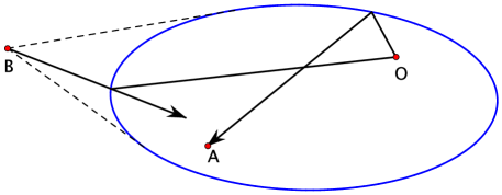
Figure 7: The curve $C_{n}$ intersects every ”line”.

This concludes the proof (which is a variation of one of the arguments given in [7]).

Let us remark that there exist at least $n+1$ $n$-bounce billiard shots from $O$ to $A$; this follows from a slight modification of a theorem of M. Farber [12].

Let us finish with a problem: Does a 4-cusp result, similar to Theorem 2, hold for more general Finsler billiards?

For example, consider a constant weak magnetic field in an oval. The billiard trajectories are arcs of a circle of radius $R$, and the weakness of the field means that the minimal curvature of the oval is greater than $1/R$ (hence the trajectories cannot touch the oval from inside). The caustic by reflection is the envelope of a 1-parameter family of circles of radius $R$, and it has two components. See Figure 8 and 9 for the first and second caustics by reflection in a circle.

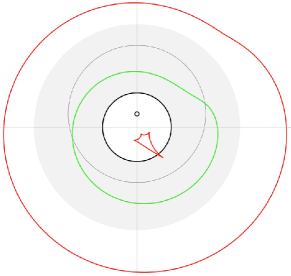
Figure 8: The first and second caustics by reflection (courtesy of G. Bor). The inner component of the caustic has four cusps, while the outer one is smooth. The green curve is the curve of centers of the Larmor circles, an analog of the curve $C_{n}$.

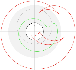
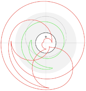
Figure 9: Same billiard with a different choice of the initial point $O$ located farther from the center of the disc.

Acknowledgment.

I am grateful to Gil Bor for numerous interesting discussions and help with computer experiments. This research was supported by NSF grant DMS-2404535 and by Simons grant TSM-00007747.

References

- [1] J. C. Álvarez Paiva. Hilbert’s fourth problem in two dimensions. MASS selecta, 165–183, Amer. Math. Soc., Providence, RI, 2003.
- [2] J. C. Álvarez Paiva. Some problems on Finsler geometry. Handbook of differential geometry. Vol. II, 1–33, Elsevier/North-Holland, Amsterdam, 2006.
- [3] A. Akopyan, R. Karasev. When different norms lead to same billiard trajectories? Eur. J. Math. 8 (2022), 1309–1312.
- [4] A. Akopyan, A. Zaslavsky. Geometry of conics. Math. World, 26. Amer. Math. Society, Providence, RI, 2007.
- [5] V. Arnold. Topological problems in the theory of wave propagation. Russian Math. Surveys 51 (1996), no. 1, 1–47.
- [6] S. Artstein-Avidan, R. Karasev, Y. Ostrover. From symplectic measurements to the Mahler conjecture. Duke Math. J. 163 (2014), 2003–2022.
- [7] G. Bor, S. Tabachnikov. On cusps of caustics by reflection: billiard variations on the four vertex theorem and on Jacobi’s last geometric statement. Amer. Math. Monthly 130 (2023), 454–467.
- [8] G. Bor, M. Spivakovsky, S. Tabachnikov. Cusps of caustics by reflection in ellipses. J. Lond. Math. Soc. 110 (2024), no. 6, Paper No. e70033.
- [9] H. Busemann. Problem IV: Desarguesian spaces in Mathematical developments arising from Hilbert problems. Proc. Sympos. Pure Math., Vol. XXVIII, Amer. Math. Soc., Providence, RI, 1976.
- [10] S.S. Chern. Finsler geometry is just Riemannian geometry without the quadratic restriction. Notices Amer. Math. Soc. 43 (1996), 959–963.
- [11] D. Faifman. A Funk perspective on billiards, projective geometry and Mahler volume. J. Differential Geom. 127 (2024), 161–212.
- [12] M. Farber. Topology of billiard problems. I, II. Duke Math. J. 115 (2002), 559–585, 587–621.
- [13] E. Gutkin, S. Tabachnikov. Billiards in Finsler and Minkowski geometries. J. Geom. Phys. 40 (2002), 277–301.
- [14] J. Itoh, K. Kiyohara. The cut loci and the conjugate loci on ellipsoids. Manuscripta Math. 114 (2004), 247–264.
- [15] A. Pogorelov. Hilbert’s Fourth Problem. A Halsted Press Book. V. H. Winston & Sons, Washington, DC; John Wiley & Sons, New York-Toronto-London, 1979.
- [16] M. Radnović. A note on billiard systems in Finsler plane with elliptic indicatrices. Publ. Inst. Math. (Beograd) 74(88) (2003), 97–101.
- [17] B. Segre. Alcune proprieta differenziali in grande delle curve chiuse sghembe. Rend. Mat. (6) 1 (1968), 237–297.
- [18] R. Sinclair. On the Last Geometric Statement of Jacobi. Experimental Math. 12 (2003), 477–485.
- [19] S. Tabachnikov. Remarks on magnetic flows and magnetic billiards, Finsler metrics and a magnetic analog of Hilbert’s fourth problem. Modern dynamical systems and applications, 233–250, Cambridge Univ. Press, 2004.
- [20] T. Waters. The conjugate locus on convex surfaces. Geom. Dedicata 200 (2019), 241–254.