Time Symmetries of Quantum Memory Improve Thermodynamic Efficiency

Abstract

Classical computations inherently require energy dissipation that increases significantly as the reliability of the computation improves. This dissipation arises when transitions between memory states are not balanced by their time-reversed counterparts. While classical memories exhibit a discrete set of possible time-reversal symmetries, quantum memory offers a continuum. This continuum enables the design of quantum memories that minimize irreversibility. As a result, quantum memory reduces energy dissipation several orders of magnitude below classical memory.

Introduction

— Computation requires energy—a fact driven home by Landauer’s recognition that “information is physical” [1]. Memory states of a computation are physically instantiated configurations of a system, meaning they must obey the laws of physics. For instance, the Second Law of thermodynamics implies that a computation’s reduction in state-space must be balanced by entropy flow (e.g., heat) into the environment to guarantee that the average entropy production is non-negative. This minimum heat cost, known as Landauer’s bound, appears to be inescapable regardless of whether the computation is classical in nature [1, 2] or quantum [3, 4, 5].

Today, practical computation requires much more energy than can be predicted from Landauer’s bound [6]. One might anticipate that this is simply a limitation of our current technology, and that with enough patient engineering, we will approach Landauer’s bound arbitrarily closely, achieving the theoretical limit of thermodynamically efficient computing. However, modern stochastic thermodynamics has found that realistic constraints like finite duration, modularity of circuits, or a lack of external driving, imply fundamentally new bounds on the heat required to drive a computation [7, 8, 9]. These advances have been achieved via equalities known as fluctuation theorems [10, 11], which generalize the Second Law inequality, and directly relate entropy production to the dynamics of a computation.

Fluctuation theorems imply that a system’s observed trajectories bound entropy production. The entropy production quantifies thermodynamic irreversibility and thus loss of energetic resources beyond Landauer’s bound [12, 13, 14, 15]. The relative probabilities of transitioning between two physical states can only be biased via an irreversible investment in thermodynamic resources. In this vein, Ref. [16] showed that non-reciprocated transitions between memory states of a computer imply divergent energetic costs as the computer becomes more reliable. However, this glosses over a nuance that can have profound implications: Time reversal symmetries of the physical states co-determine thermodynamic irreversibility of an observed trajectory. While this dependence on time-reversal symmetries is known in nonequilibrium thermodynamics [17], the implications for the energetics of computation remain largely unexplored besides Refs. [16, 18]. Indeed, the thermodynamic irreversibility of a computation depends sensitively on the time-reversal symmetries of memory elements used in the computation. And, as we will show, quantum can help.

For time-even variables like DNA nucleotide sequences, time reversal doesn’t affect the encoded information (thymine remains thymine in reverse time). However, information in a hard disk drive is encoded in magnetic moments, which flip sign under time reversal, mapping the logical elements ${\color[rgb]{0,0,1}{\bm{\mathtt{0}}}}\mapsto{\color[rgb]{0,0,1}{\bm{\mathtt{1}}}}$ and ${\color[rgb]{0,0,1}{\bm{\mathtt{1}}}}\mapsto{\color[rgb]{0,0,1}{\bm{\mathtt{0}}}}$. Memory devices which change under time reversal, like magnetic storage, are time-odd [19, 20]. The flexibility of time-symmetries of memory appears to allow the designer of a computational circuit to choose an appropriate substrate, that effectively minimizes the thermodynamic irreversibility of the computation [18].

However, even with the flexibility to design time-symmetries of classical memory, logical irreversibility requires divergent dissipation in the limit of increasing reliability  [18]. It is in this context that we show a considerable energetic advantage enabled by quantum memory elements. Unlike classical time-reversal, which is limited to discrete involutions, quantum time-reversal operations correspond to anti-unitary operators [21, 22, 23]. In the following, we show that the additional flexibility of quantum memory allows us to implement logically irreversible computations without divergent dissipation. Thus, there is a significant thermodynamic advantage to performing fundamental logical operations with quantum memory.

Thermodynamic Bound on Computation

— Consider a computation, which is instantiated within a memory-storing system $\mathbf{S}$ with reduced density matrix $\rho_{t}$ at time $t$ in contact with a thermal environment $\mathbf{E}$ with reduced density matrix $\rho_{t}^{\text{env}}$ that starts in local equilibrium $\rho_{0}^{\text{env}}=\bigotimes_{b}\bm{\pi}_{b}$, where $\bm{\pi}_{b}$ is the equilibrium distribution (e.g., canonical or grand canonical) for environmental bath $b$. The computation is implemented through a unitary $U_{\lambda_{0:\tau}}$ applied to the joint system–environment supersystem, where $\lambda_{0:\tau}\equiv\lambda_{0}\cdots\lambda_{\tau}$ is the control sequence. This is the unitary dynamics that results from applying Hamiltonian $H_{\lambda_{t}}$ using control parameter $\lambda_{t}$ at every time $t$ within the computation interval $t\in[0,\tau]$. The environment adds additional degrees of freedom such that the operation over the system $\mathbf{S}$ need not be unitary and information preserving. Generally, the net operation over the system $\mathbf{S}$ can be expressed as a completely positive and trace preserving (CPTP) operation $O_{\lambda_{0:\tau}}$. This is a general framework for quantum open-system transformations since, via Stinespring’s dilation theorem, every CPTP operation on the system can be implemented through a unitary transformation on a larger space [24, 25, 26].

On the joint system–environment supersystem, we derive a statement of microscopic reversibility in App. B:

$$\Pr(z\stackrel{{\scriptstyle\lambda_{0:\tau}}}{{\mapsto}}z^{\prime})=\Pr(z^{\prime\dagger}\stackrel{{\scriptstyle\lambda_{0:\tau}^{R}}}{{\mapsto}}z^{\dagger})$$ (1)

which, in turn, allows us to derive thermodynamic consequences for computational transitions on the memory subsystem. Eq. (1) says that the probability that (i) a measurement of the joint state would yield $z^{\prime}$ at the end of a protocol $\lambda_{0:\tau}$ (given the initial quantum state $z$) is the same as (ii) the probability of obtaining the measurement outcome $z^{\dagger}$—the time-reversal of the joint state $z$—at the end of the time-reversed protocol $\lambda^{R}_{0:\tau}$ if the supersystem begins in the time-reversed state $z^{\prime\dagger}$.

We connect the dynamics of the computation $O_{\lambda_{0:\tau}}$ to thermodynamics via a quantum detailed fluctuation theorem (QDFT) [27, 17, 28]. We derive a general QDFT in App. C that directly relates entropy production $\Sigma$ in a quantum transformation to the forward and reverse measurement probabilities on the system alone. The generality of this theorem is tied to the fact that it accommodates a system in contact with arbitrarily many baths that begin in local equilibrium, like heat and particle baths that each start as a grand canonical ensemble. As such, the first contribution to the total entropy production of a system $\mathbf{S}$ is the entropy flow $\Phi$, due to particle and heat flow into the environment,

$$\Phi=\sum_{b}\frac{Q_{b}-\mu_{b}\Delta N_{b}}{T_{b}},$$ (2)

where each reservoir is indexed by $b$ with chemical potential $\mu_{b}$ and temperature $T_{b}$ [29]. This admits a wide variety of possible scenarios for nonequilibrium computation, and follows roughly the same logic as Jarzynski’s original Hamiltonian derivation of a detailed fluctuation theorem [11].

The total entropy production also includes the change in system surprisal $\Delta S_{s_{0},s_{\tau}}=k_{\text{B}}\ln\braket{s_{0}|\rho_{0}|s_{0}}-k_{\text{B}}\ln\braket{s_{\tau}|\rho_{\tau}|s_{\tau}}$, where $k_{\text{B}}$ is Boltzmann’s constant. $\Sigma\equiv\Phi_{s_{0},s_{\tau}}+\Delta S_{s_{0},s_{\tau}}$ captures the entropy production of a particular measurement trajectory $s_{0}\rightarrow s_{\tau}$, because it produces the the change in von Neumann entropy of the system plus the entropy flow to the environment when averaged over all state sequences [29, 30, 31]. Note that this entropy production is specifically from the initial post-measurement state $\sum_{s_{0}}\Pi_{s_{0}}\rho_{0}\Pi_{s_{0}}$ to the final post-measurement state $\sum_{s_{\tau}}\Pi_{s_{\tau}}\rho_{\tau}\Pi_{s_{\tau}}$. As App. C shows, the entropy production for a state transition $s_{0}\rightarrow s_{\tau}$ is bounded below by computational entropy production

$$\Sigma^{\text{comp}}_{s_{0},s_{\tau}}\leq\Sigma_{s_{0},s_{\tau}}.$$ (3)

The subscript $s_{0},s_{\tau}$ indicates the average of all measured trajectories for which the system starts in $s_{0}$ and ends in $s_{\tau}$. This measure quantifies the irreversibility of a state transition

$$\Sigma^{\text{comp}}_{s_{0},s_{\tau}}\equiv k_{\text{B}}\ln\frac{f(s_{0},s_{\tau})}{r(s_{0},s_{\tau})},$$ (4)

in terms of the forward transition probability $f(s_{0},s_{\tau})$ and reverse transition probability $r(s_{0},s_{\tau})$. Observed irreversibility in a system typically implies dissipation [32, 33, 34], and $\Sigma^{\text{comp}}_{s_{0},s_{\tau}}$ is the unavoidable entropy production associated with the computation when $s_{0}\rightarrow s_{\tau}$.

Crucially in evaluating irreversibility, the time-reversed transition probability $r(s_{0},s_{\tau})$ involves not only the time-reversed state sequence, but also the physical states $s_{0}^{\dagger}$ and $s_{\tau}^{\dagger}$ induced by the time-reversal operator acting on states $s_{0}$ and $s_{\tau}$. Specifically, the forward probability $f(s_{0},s_{\tau})$ is that of measuring $s_{0}$ then $s_{\tau}$ after applying the forward control $\lambda_{0:\tau}$. The reverse probability $r(s_{0},s_{\tau})$ is that of measuring $s_{\tau}^{\dagger}$ then $s_{0}^{\dagger}$ after applying the reverse control sequence $\lambda^{R}_{0:\tau}$ (where $\lambda_{t}^{R}$ applies the time-reversal of $H_{\lambda_{\tau-t}}$), assuming that the initial state density is the same as the time reversal of the final state of the forward experiment [35].

We can exactly calculate the computational entropy production for a quantum computation using Eq. (4). Given the initial density $\rho_{0}$, the forward computation $O_{\lambda_{0:\tau}}$, the final density $\rho_{\tau}=O_{\lambda_{0:\tau}}(\sum_{s_{0}}\Pi_{s_{0}}\rho_{0}\Pi_{s_{0}})$, and the reverse computation $O_{\lambda^{R}_{0:\tau}}$, we can exactly calculate the transition probabilities:

$$f(s_{0},s_{\tau}) =\text{Tr}\left[\Pi_{s_{\tau}}O_{\lambda_{0:\tau}}(\Pi_{s_{0}})\right]p_{0}(s_{0})$$ (5)

$$r(s_{0},s_{\tau}) =\text{Tr}\left[\Pi_{s_{0}^{\dagger}}O_{\lambda^{R}_{0:\tau}}(\Pi_{s_{\tau}^{\dagger}})\right]p_{\tau}(s_{\tau}).$$ (6)

Here, $\Pi_{s}\equiv|s\rangle\langle s|$ is the projector onto the pure system state $|s\rangle$, $p_{0}(s_{0})\equiv\text{Tr}\left[\Pi_{s_{0}}\rho_{0}\right]$ is the initial probability of $s_{0}$, and $p_{\tau}(s_{\tau})\equiv\text{Tr}\left[\Pi_{s_{\tau}}\rho_{\tau}\right]$ is the final probability of $s_{\tau}$. The time reversal of a state comes from the anti-unitary time-reversal operator

$$|s^{\dagger}\rangle\equiv\Theta|s\rangle.$$ (7)

The way in which the states change under time reversal directly affects the lower bound on entropy production.

Time-Symmetric Control of Classical Computation

— Practical computing paradigms operate under time-symmetric control [16, 36]. Time-symmetric control is also assumed for nonequilibrium steady state biochemical computing [37, 33], thermodynamic clocks [38], thermodynamic uncertainty relations [39, 40], and thermodynamic cost of waiting time distributions [41]. The control trajectory is the same under time reversal $\lambda_{0:\tau}=\lambda_{0:\tau}^{R}$. This is most clear for something like a laptop computer which runs its program through the constant nonequilibrium driving of the battery. This remains true even if we consider the computational memory system driven by the periodic $\sim$3GHz clock that marches the Markovian memory dynamics forward. For quantum computers too, we can expect a constant or periodic influence to march the computation forward, whereas a time-asymmetric driving signal would come with its own thermodynamic cost. In this case we can simply identify a single CPTP operation for forward and reverse $O=O_{\lambda_{0:\tau}}=O_{\lambda^{R}_{0:\tau}}$, which determines the computational entropy production of a particular state sequence

$$\Sigma^{\text{comp}}_{s_{0},s_{\tau}}=k_{\text{B}}\ln\frac{\text{Tr}\left[\Pi_{s_{\tau}}O(\Pi_{s_{0}})\right]p_{0}(s_{0})}{\text{Tr}\left[\Pi_{s_{0}^{\dagger}}O(\Pi_{s_{\tau}^{\dagger}})\right]p_{\tau}(s_{\tau})}~.$$ (8)

To appreciate the flexibility of the time-symmetries of quantum mechanics, consider first a classical computation that is specified by a Markov channel $M_{s_{0}\rightarrow s_{\tau}}\equiv\Pr(S_{\tau}=s_{\tau}|S_{0}=s_{0})$, which specifies the probability of final state $s_{\tau}$ given the initial state $s_{0}$, with $S_{t}$ denoting the random variable for for the system at time $t$ [42]. We can implement this classical computation as a CPTP map

$$O(\circ)=\sum_{s^{\prime}_{0},s^{\prime}_{\tau}}M_{s^{\prime}_{0}\rightarrow s^{\prime}_{\tau}}\Pi_{s^{\prime}_{\tau}}\text{Tr}\left[\Pi_{s^{\prime}_{0}}\circ\right].$$ (9)

This operation measures in the original computational basis, updates according to the stochastic channel $M$, then outputs a state in the same computational basis.

The resulting computational entropy production

$$\Sigma^{\text{comp}}_{s_{0},s_{\tau}} =k_{\text{B}}\ln\frac{M_{s_{0}\rightarrow s_{\tau}}p_{0}(s_{0})}{M^{\dagger}_{s_{\tau}^{\dagger}\rightarrow s_{0}^{\dagger}}p_{\tau}(s_{\tau})}~,$$ (10)

with reverse transition matrix in the denominator

$$M^{\dagger}_{s_{\tau}^{\dagger}\rightarrow s_{0}^{\dagger}}\equiv\sum_{s^{\prime}_{0},s^{\prime}_{\tau}}M_{s^{\prime}_{0}\rightarrow s^{\prime}_{\tau}}p(s_{0}^{\prime}|s^{\dagger}_{\tau})p(s^{\dagger}_{0}|s_{\tau}^{\prime})~,$$ (11)

depends on the overlap between states and their time reversals since $p(s^{\dagger}|s^{\prime})=p(s^{\prime}|s^{\dagger})=|\langle s^{\prime}|s^{\dagger}\rangle|^{2}$ is both the probability of measuring the time reversed state $|s^{\dagger}\rangle$ given the state $|s^{\prime}\rangle$, and the probability of measuring $|s^{\prime}\rangle$ given the time reversed state $|s^{\dagger}\rangle$. $M^{\dagger}_{s_{\tau}^{\dagger}\rightarrow s_{0}^{\dagger}}$ is the probability of measuring $|s_{0}^{\dagger}\rangle$ given that the system is prepared in state $|s_{\tau}^{\dagger}\rangle$, measured in the forward-time computational basis, then transformed by the Markov channel $M$. We evaluate the average computational entropy production over all input-output combinations $s_{0}$ and $s_{\tau}$ to evaluate the overall minimum thermodynamic efficiency of a computation

$$\langle\Sigma^{\text{comp}}\rangle=\sum_{s_{0},s_{\tau}}\Pr(S_{0}=s_{0},S_{\tau}=s_{\tau})\Sigma^{\text{comp}}_{s_{0},s_{\tau}}~.$$ (12)

Time-Reversal Operators

— There are many different time-reversal symmetries depending on how information is physically encoded. In classical physics, these symmetries correspond to involutions, which are functions between elements of the state space $\Theta:\mathcal{S}\rightarrow\mathcal{S}$ that are their own inverse $\Theta(\Theta(s))=s$. This guarantees that reversing the time twice takes you back to where you started. Two fundamental examples are time-even positional and time-odd momentum time-reversal,

$$\Theta(x)=x\text{, }\Theta(p)=-p,$$ (13)

reflecting that positions are preserved while momentum flips sign under time reversal.

Quantum time-reversals are much more flexible than classical, because they are antiunitary operators [21, 22, 23]. Such operators are antilinear, meaning that they conjugate when they commute with complex numbers $\Theta c=c^{*}\Theta$. In essence, this means that it can be expressed as the composition of a basis-dependent unitary $U$ and a complex conjugation operator $K$

$$\Theta=UK.$$ (14)

Unlike linear operators, the action of the complex conjugation operator depends on the particular choice of basis in which you choose to represent the memory states. It conjugates coefficients $Kc=c^{*}K$, but leaves basis elements fixed: $K|s\rangle=|s\rangle$ [43]. We use this to our advantage in the next section, where we introduce energy-efficient computations with quantum memory.

Quantum Thermodynamic Advantage

— Quantum memory offers a divergent thermodynamic advantage for logically irreversible computation. Consider the most basic irreversible computation: erasure. The erasure resets a binary memory $\mathcal{S}=\{{\color[rgb]{0,0,1}{\bm{\mathtt{0}}}},{\color[rgb]{0,0,1}{\bm{\mathtt{1}}}}\}$ to the reset state, which we will choose to be ${\color[rgb]{0,0,1}{\bm{\mathtt{0}}}}$ without loss of generality. The components of such an operation are

$$M^{\text{erase}}_{s\rightarrow s^{\prime}}=\delta_{0,s^{\prime}}(1-\epsilon)+(1-\delta_{0,s^{\prime}})\frac{\epsilon}{|\mathcal{S}|-1},$$ (15)

where $\epsilon\ll 1$ specifies the error rate and $|\mathcal{S}|$ is the dimension of the system.

In the special case where memory is classical, we have only two time-reversal symmetries:

1. Time-even ${\color[rgb]{0,0,1}{\bm{\mathtt{0}}}}^{\dagger}={\color[rgb]{0,0,1}{\bm{\mathtt{0}}}}$ and ${\color[rgb]{0,0,1}{\bm{\mathtt{1}}}}^{\dagger}={\color[rgb]{0,0,1}{\bm{\mathtt{1}}}}$.

2. Time-odd ${\color[rgb]{0,0,1}{\bm{\mathtt{0}}}}^{\dagger}={\color[rgb]{0,0,1}{\bm{\mathtt{1}}}}$ and ${\color[rgb]{0,0,1}{\bm{\mathtt{1}}}}^{\dagger}={\color[rgb]{0,0,1}{\bm{\mathtt{0}}}}$.

In the time-even case, the lower bound on entropy production found in Eq. (12) is

$$\frac{\langle\Sigma^{\text{comp}}\rangle}{k_{B}}= \operatorname{H}[S_{\tau}]-\operatorname{H}[S_{0}]+(p_{0}({\color[rgb]{0,0,1}{\bm{\mathtt{1}}}})-\epsilon)\ln\frac{1-\epsilon}{\epsilon}~.$$ (16)

In the time-odd case, the same computational entropy production is

$$\frac{\langle\Sigma^{\text{comp}}\rangle}{k_{B}}=\operatorname{H}[S_{\tau}]-\operatorname{H}[S_{0}]+(p_{0}({\color[rgb]{0,0,1}{\bm{\mathtt{0}}}})-\epsilon)\ln\frac{1-\epsilon}{\epsilon}.$$ (17)

In either case, as the reliability increases, the error goes to zero $\epsilon\rightarrow 0$, and the error is dominated by a term with the divergent coefficient $\ln(1/\epsilon)$. As a result, classically implemented erasure must dissipate divergent energy as reliability increases [16].

By contrast, let’s consider the entropy production of quantum positional information bearing degrees of freedom, which are invariant under time reversal [43]

$$\Theta|x_{0}\rangle=|x_{0}\rangle\text{, }\;\Theta|x_{1}\rangle =|x_{1}\rangle.$$ (18)

This is in line with quantum computing protocols that store information spatially, for instance in metastable double-wells [44]. In this basis, $\Theta$ operates as the complex conjugate operator $\Theta=K$. However, we can also consider a new orthonormal basis $\{|a\rangle,|b\rangle\}$ which is a superposition of these states

$$|a\rangle\equiv\frac{|x_{0}\rangle+i|x_{1}\rangle}{\sqrt{2}}\text{, }\;|b\rangle\equiv\frac{|x_{0}\rangle-i|x_{1}\rangle}{\sqrt{2}}$$ (19)

Upon time reversal, the states swap:

$$\Theta|a\rangle=|b\rangle\text{, }\;\Theta|b\rangle=|a\rangle.$$ (20)

If we choose the memory to be represented in this basis ($|{\color[rgb]{0,0,1}{\bm{\mathtt{0}}}}\rangle=|a\rangle$ and $|{\color[rgb]{0,0,1}{\bm{\mathtt{1}}}}\rangle=|b\rangle$), then we have the familiar time-odd time symmetry described above ($\Theta|{\color[rgb]{0,0,1}{\bm{\mathtt{0}}}}\rangle=|{\color[rgb]{0,0,1}{\bm{\mathtt{1}}}}\rangle$ and $\Theta|{\color[rgb]{0,0,1}{\bm{\mathtt{1}}}}\rangle=|{\color[rgb]{0,0,1}{\bm{\mathtt{0}}}}\rangle$). With these two bases in the same Bloch sphere, we are able to explore the two relevant classical time symmetries.

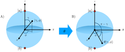
Figure 1: Time reversal on the Bloch sphere is a reflection. The state $|\gamma,\varphi\rangle$ shown in A) is reflected across the $xy$-plane to produce the time reversal in $\Theta|\gamma,\varphi\rangle=|\pi-\gamma,\varphi\rangle$ in B).

We can explore many more time-reversal symmetries by considering the continuous variety of pure states on the Bloch sphere as shown in Fig. 1. These can be parametrized by the angle $\gamma$ from $|a\rangle$ and the azimuth $\varphi$

$$|\gamma,\varphi\rangle=\cos(\gamma/2)|a\rangle+e^{i\varphi}\sin(\gamma/2)|b\rangle.$$ (21)

The natural orthogonal state to complete this basis is $|\gamma+\pi,\varphi\rangle$, which is on the opposite side of the Bloch sphere. Applying the time-reversal operator yields

$$\Theta|\gamma,\varphi\rangle=e^{-i\varphi}|\pi-\gamma,\varphi\rangle.$$ (22)

In essence, the time reversal is a reflection in the Bloch sphere across the plane that corresponds to the angle $\gamma=\pi/2$ as shown in Fig. 1.

To identify the quantum thermodynamic advantage, we consider the angle in the Bloch sphere $\gamma=\pi/4$ and identify the computational states:

$$|{\color[rgb]{0,0,1}{\bm{\mathtt{0}}}}\rangle=|\pi/4,\varphi\rangle\text{, }\;|{\color[rgb]{0,0,1}{\bm{\mathtt{1}}}}\rangle=|\pi+\pi/4,\varphi\rangle.$$ (23)

The time-reversed states are

$$|{\color[rgb]{0,0,1}{\bm{\mathtt{0}}}}^{\dagger}\rangle=|\pi-\pi/4,\varphi\rangle\text{, }\;|{\color[rgb]{0,0,1}{\bm{\mathtt{1}}}}^{\dagger}\rangle=|-\pi/4,\varphi\rangle.$$ (24)

In order to calculate the entropy production associated with an erasure, we calculate the overlap between each combination of $|s^{\dagger}\rangle$ and $|s^{\prime}\rangle$, which turns out to be the same for all state pairs:

$$p(s^{\dagger}|s^{\prime})=|\langle s^{\prime}|s^{\dagger}\rangle|^{2} =1/|\mathcal{S}|~.$$ (25)

The size of the alphabet in this case is $|\mathcal{S}|=2$. The memory basis and its time reversal are mutually unbiased [45]. In this case, and more broadly for a system of any size where the time reversal satisfies the relation $|\langle s^{\prime}|s^{\dagger}\rangle|^{2}=\frac{1}{|\mathcal{S}|}$ the entropy production simplifies to

$$\Sigma^{\text{comp}}_{s_{0},s_{\tau}}=k_{\text{B}}\ln|\mathcal{S}|+k_{\text{B}}\ln\Pr(S_{0}=s_{0}|S_{\tau}=s_{\tau}).$$ (26)

The resulting average computational entropy production is

$$\langle\Sigma^{\text{comp}}\rangle=k_{\text{B}}\ln|\mathcal{S}|-k_{\text{B}}\operatorname{H}[S_{0}|S_{\tau}],$$ (27)

where $\operatorname{H}[S_{0}|S_{\tau}]$ is the Shannon entropy of the initial state conditioned on the final state (see App. A). This entropy production never diverges, unlike computation instantiated on classical memory, whose dissipation necessarily diverges for reliable logically irreversible transformations [18].

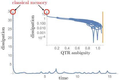
Figure 2: Thermodynamic Quantum Advantage: The dissipation ($\langle\Sigma^{\text{comp}}\rangle$ shown in units of $k_{\text{B}}$) of a three-state erasure is high ($\sim 35k_{\text{B}}$) for the classical case (identified with red circles), but is typically orders of magnitude lower ($<k_{\text{B}}$), going as low as $10^{-4}k_{\text{B}}$. Dissipation is initially very high, because the system is prepared in a classical basis, but the dissipation quickly reduces as the basis evolves unitarily. The dissipation fluctuates around values that are orders of magnitude lower than the limit for classical memory as the evolution explores quantum memory states.
(Inset): The reduction in dissipation roughly corresponds to increasing QTR ambiguity $\operatorname{H}[S^{\dagger}|S]$. The dissipation is nearly minimal for maximal values of QTR ambiguity. The orange line indicates the upper limit of the QTR ambiguity.

Exploring Efficiency of Time Symmetries

— The probability of the time-reversed state given the initial state $p(s^{\dagger}|s^{\prime})=|\langle s^{\dagger}|s^{\prime}\rangle|^{2}$ is the source of the quantum advantage for these irreversible classical computations. Unlike classical time reversals, for which the probability is highly peaked around a particular involution $p(s^{\dagger}|s^{\prime})=\delta_{s,f(s^{\prime})}$, quantum time reversals can have high ambiguity in the time-reversed state. We saw this above, where the maximally uncertain distribution and mutually unbiased basis ($p(s^{\dagger}|s^{\prime})=\frac{1}{|\mathcal{S}|}$) allows us to implement thermodynamically efficient erasure.

While we were able to find the mutually unbiased time-reversed bases for a two-state computation, it’s not clear to us how to do this in general. Thus, we explore different quantum bases for computation numerically, and compare the dissipation to the ambiguity in the time-reversed state (assuming uniform state density $p(s)=1/|\mathcal{S}|$):

$$\operatorname{H}[S^{\dagger}|S]\equiv-\sum_{n,n^{\prime}}p(s^{\dagger}_{n^{\prime}}|s_{n})p(s_{n})\ln p(s^{\dagger}_{n^{\prime}}|s_{n})~.$$ (28)

We call this the QTR ambiguity (QTR stands for Quantum Time-Reversal). The QTR ambiguity is zero iff the memory basis is classical and time-reversal is a permutation. This measure effectively quantifies the “quantumness” of the time-reversal. In the case where the QTR ambiguity is zero, we retain the classical result that entropy production diverges for a reliable erasure operation.

We explore different quantum bases for information storage numerically as discussed in App. D. The system begins in a classical basis, then it evolves according to the Schrodinger equation, creating quantum coherence in the memory. The error rate of the computation is $\epsilon=10^{-26}$, to parallel CMOS logic circuits [46, 16]. Fig. 2 shows that the computational entropy production begins at a high-point, where the time-reversal is classical, and it quickly reduces by orders of magnitude as the basis evolves to take advantage of quantum effects. For comparison the QTR ambiguity begins at zero, but increases roughly as the efficiency of the computation increases.

Conclusion

— Irreversibility in a computation incurs entropy production. This irreversibility depends on both the logical operation as well as the time-reversal symmetries of the underlying hardware. We see that quantum hardware allows us to circumnavigate divergent dissipation that occurs in logically irreversible operations. Quantum memory offers orders-of-magnitude improvements in thermodynamic efficiency beyond classical implementations of the same computation.

Appendix A Random Variable for Thermodynamic Experiments

Random variables are useful for accurately expressing complex multipartite probabilities and their relationships. Generally, we will use lower-case letters like $a$ and $b$ for realizations of probability distributions, and upper-case letters like $A$ and $B$ for their random variables, such that we can express marginal probabilities, joint probabilities, and conditionals efficiently

$$\text{Marginal probability of }A\text{ realizing }a\text{: } \Pr(A=a)$$ (29)

$$\text{Joint probability of }A\text{ and }B\text{ realizing }a\text{ and }b\text{: } \Pr(A=a,B=b)$$ (30)

$$\text{Conditional probability of }A\text{ realizing }a\text{ given that }B\text{ realizes }b\text{: } \Pr(A=a|B=b)\equiv\frac{\Pr(A=a,B=b)}{\Pr(B=b)}.$$ (31)

This also allows us to easily and efficiently express Shannon entropies (measured in nats)

$$\operatorname{H}[A]\equiv-\sum_{a\in\mathcal{A}}\Pr(A=a)\ln\Pr(A=a),$$ (32)

and conditional uncertainty

$$\operatorname{H}[A|B]\equiv\operatorname{H}[A,B]-\operatorname{H}[B].$$ (33)

Appendix B Microscopic Reversibility of Hamiltonian Control

Quantum dynamics guarantees specific relationships between the probabilities of forward experiments and reverse experiments. Specifically, if we apply Hamiltonian control $H_{\lambda_{t}}$ to a system $\mathcal{Z}$ (which in our framework is the system–environment supersystem), indexed by a vector of control parameters $\lambda_{t}$ over the time interval $[0,\tau]$, the net result is a unitary time evolution operator. Without loss of generality, we can simplify the analysis by considering a sequence of $N+1$ discrete time-steps of duration $\Delta t=\tau/N$, marked by the sequence of times $t_{n}=n\tau/N$, and take the limit of $N\to\infty$ for continuous-time control. We then obtain the unitary time evolution operator and its inverse

$$U_{\lambda_{0:\tau}} =\lim_{N\to\infty}\prod_{n=0}^{N}e^{-i\Delta tH_{\lambda_{t_{n}}}/\hbar}$$ (34)

$$U_{\lambda_{0:\tau}}^{-1} =\lim_{N\to\infty}\prod_{n=0}^{N}e^{i\Delta tH_{\lambda_{\tau-t_{n}}}/\hbar}~,$$ (35)

where the time ordering of multiplication is implied.

We can evaluate the probabilities of measurement outcomes for the final state $z_{\tau}$ given the initial state was $z_{0}$ and we perform the experiment with forward control $\lambda_{0:\tau}$:

$$\Pr(Z_{\tau}=z_{\tau}|Z_{0}=z_{0},\Lambda_{0:\tau}=\lambda_{0:\tau})=|\langle z_{\tau}|U_{\lambda_{0:\tau}}|z_{0}\rangle|^{2}.$$ (36)

Note that we have explicitly conditioned on the control parameter sequence $\lambda_{0:\tau}$ since we consider distributions from multiple different experiments.

For comparison, we evaluate the probabilities of transitions under reverse control, where we time reverse the sequence of control parameters, and we conjugate each control parameter

$$\lambda^{R}_{0:\tau}\equiv\lambda_{\tau}^{\dagger}\cdots\lambda_{0}^{\dagger}.$$ (37)

Time-reversal of the control parameter time-reverses the Hamiltonian $H_{\lambda^{\dagger}}=\Theta H_{\lambda}\Theta^{-1}$. This allows us to generalize beyond Hamiltonians that are time-reversal invariant, allowing for the possibility that $\Theta H\neq H\Theta$ [17, 23]. In the classical context, time-reversal of the Hamiltonian flips the sign of time-odd parameters like magnetic fields. However, quantum time-reversal is more nuanced. We can evaluate the probability of measurement outcome $z_{0}^{\dagger}$ after applying the control $\lambda^{R}_{0:\tau}$, given that the initial state was $z_{\tau}^{\dagger}$:

$$\Pr(Z_{\tau}=z_{0}^{\dagger}|Z_{0}=z_{\tau}^{\dagger},\Lambda_{0:\tau}=\lambda^{R}_{0:\tau}) =|\langle z_{0}^{\dagger}|U_{\lambda^{R}_{0:\tau}}|z_{\tau}^{\dagger}\rangle|^{2}.$$ (38)

To evaluate this, the unitary evolution associated with time-reversed control is

$$U_{\lambda^{R}_{0:\tau}} =\lim_{N\to\infty}\prod_{n=0}^{N}e^{-i\Delta tH_{\lambda_{\tau-t_{n}}^{\dagger}}/\hbar}$$ (39)

$$=\lim_{N\to\infty}\prod_{n=0}^{N}e^{-i\Delta t\Theta H_{\lambda_{\tau-t_{n}}}\Theta^{-1}/\hbar}$$ (40)

$$=\lim_{N\to\infty}\prod_{n=0}^{N}e^{\Theta(i\Delta tH_{\lambda_{\tau-t_{n}}}/\hbar)\Theta^{-1}}.$$ (41)

We can further simplify by noting that the exponential of a time-reverse operator is the time reversal of the exponential of that operator

$$e^{\Theta\hat{O}\Theta^{-1}} =\sum_{j=0}^{\infty}\frac{(\Theta\hat{O}\Theta^{-1})^{j}}{j!}$$ (42)

$$=\Theta\sum_{j=0}^{\infty}\frac{\hat{O}^{j}}{i!}\Theta^{-1}$$ (43)

$$=\Theta e^{\hat{O}}\Theta^{-1},$$ (44)

such that

$$U_{\lambda^{R}_{0:\tau}} =\lim_{N\to\infty}\prod_{n=0}^{N}\Theta e^{i\Delta tH_{\lambda_{\tau-t_{n}}}/\hbar}\Theta^{-1}$$ (45)

$$=\Theta U_{\lambda_{0:\tau}}^{\dagger}\Theta^{-1}.$$ (46)

Note that this is more general than the expression $U\Theta=\Theta U^{\dagger}$ that applies for time-reversal invariant Hamiltonians that obey $H\Theta=\Theta H$ [17]. Plugging this into the

$$\Pr(Z_{\tau}=z_{0}^{\dagger}|Z_{0}=z_{\tau}^{\dagger},\Lambda_{0:\tau}=\lambda^{R}_{0:\tau}) =\lim_{N\to\infty}|\langle z_{0}^{\dagger}|\prod_{n=0}^{N}\Theta e^{i\Delta tH_{\lambda_{\tau-t_{n}}}/\hbar}\Theta^{-1}|z_{\tau}^{\dagger}\rangle|^{2}$$ (47)

$$=|\langle z_{0}^{\dagger}|\Theta U^{\dagger}_{\lambda_{0:\tau}}\Theta^{-1}\Theta|z_{\tau}\rangle|^{2}$$ (48)

$$=|\langle z_{0}^{\dagger}|\Theta U^{\dagger}_{\lambda_{0:\tau}}|z_{\tau}\rangle|^{2}.$$ (49)

Because time reversal is an antiunitary operator $\langle a^{\dagger}|b^{\dagger}\rangle=(\langle a|b\rangle)^{*}$. Therefore, $|\langle b^{\dagger}|\Theta|a\rangle|^{2}=|\langle b|a\rangle|^{2}$, and we have the condition of microscopic reversibility

$$\Pr(Z_{\tau}=z_{0}^{\dagger}|Z_{0}=z_{\tau}^{\dagger},\Lambda_{0:\tau}=\lambda^{R}_{0:\tau}) =|\langle z_{0}^{\dagger}|\Theta U^{\dagger}_{\lambda_{0:\tau}}|z_{\tau}\rangle|^{2}$$ (50)

$$=|\langle z_{\tau}|U_{\lambda_{0:\tau}}|z_{0}\rangle|^{2}$$ (51)

$$=\Pr(Z_{\tau}=z_{\tau}|Z_{0}=z_{0},\Lambda_{0:\tau}=\lambda_{0:\tau})~.$$ (52)

In the main text, we write Eq. (52) more succinctly as

$$\Pr(z\stackrel{{\scriptstyle\lambda_{0:\tau}}}{{\mapsto}}z^{\prime})=\Pr(z^{\prime\dagger}\stackrel{{\scriptstyle\lambda_{0:\tau}^{R}}}{{\mapsto}}z^{\dagger})~.$$ (53)

We can further generalize this idea by constructing forward and reverse experiments that are composed of a trajectory of measurements, potentially in different measurement bases and at arbitrary times, with Hamiltonian control interspersed throughout.

We now show that $U_{\lambda_{t:t^{\prime}}}^{\dagger}=\Theta^{-1}U_{\lambda_{t:t^{\prime}}^{R}}\Theta$ and $U_{\lambda_{t:t^{\prime}}}=\Theta^{-1}U_{\lambda_{t:t^{\prime}}^{R}}^{\dagger}\Theta$ together imply a quantum version of microscopic reversibility, applicable to any unitary time evolution interrupted by arbitrary projective measurements at times $\mathcal{T}\subset(0,\tau)$:

$$\Pr_{\lambda_{0:\tau},\mathcal{M}_{\mathcal{T}}}(Z_{\tau}=z^{\prime},\mathcal{M}_{\mathcal{T}}=m_{1}m_{2}\dots m_{|\mathcal{T}|}|Z_{0}=z)=\Pr_{\lambda_{0:\tau}^{R},\mathcal{M}_{\mathcal{\tilde{T}}}}(Z_{\tau}=\Theta z,\mathcal{M}_{\mathcal{\tilde{T}}}=\tilde{m}_{|\mathcal{T}|}\dots\tilde{m}_{2}\tilde{m}_{1}|Z_{0}=\Theta z^{\prime})~,$$ (54)

where $\tilde{\mathcal{T}}=(\tau-t)_{t\in\mathcal{T}}$. The set of projectors $\{\Pi_{m}\}_{m}$ used at time $t\in\mathcal{T}$ in the forward protocol are arbitrary, except that they satisfy the typical partitioning of the joint state space: $\sum_{m}\Pi_{m}=I$. In particular, the measurement projector $\Pi_{m}$ has arbitrary rank in an arbitrary basis. The technical steps parallel the earlier derivation without measurements.

$$\Pr_{\lambda_{0:\tau},\mathcal{M}_{\mathcal{T}}} (Z_{\tau}=z^{\prime},\mathcal{M}_{\mathcal{T}}=m_{1}m_{2}\dots m_{N}|Z_{0}=z)$$

$$=\text{tr}\bigl{(}\ket{z^{\prime}}\bra{z^{\prime}}U_{\lambda_{t_{|\mathcal{T}|}:\tau}}\Pi_{m_{|\mathcal{T}|}}\dots\Pi_{m_{2}}U_{\lambda_{t_{1}:t_{2}}}\Pi_{m_{1}}U_{\lambda_{0:t_{1}}}\ket{z}\bra{z}U_{\lambda_{0:t_{1}}}^{\dagger}\Pi_{m_{1}}U_{\lambda_{t_{1}:t_{2}}}^{\dagger}\Pi_{m_{2}}\dots\Pi_{m_{|\mathcal{T}|}}U_{\lambda_{t_{|\mathcal{T}|}:\tau}}^{\dagger}\bigr{)}$$ (55)

$$=\text{tr}\bigl{(}\ket{z^{\prime}}\bra{z^{\prime}}\Theta^{-1}U_{\lambda_{t_{|\mathcal{T}|}:\tau}^{R}}^{\dagger}\Theta\Pi_{m_{|\mathcal{T}|}}\dots\Pi_{m_{2}}\Theta^{-1}U_{\lambda_{t_{1}:t_{2}}^{R}}^{\dagger}\Theta\Pi_{m_{1}}\Theta^{-1}U_{\lambda_{0:t_{1}}^{R}}^{\dagger}\Theta\ket{z}\bra{z}\Theta^{-1}U_{\lambda_{0:t_{1}}^{R}}\Theta\Pi_{m_{1}}\Theta^{-1}U_{\lambda_{t_{1}:t_{2}}^{R}}\Theta\Pi_{m_{2}}\dots\Pi_{m_{|\mathcal{T}|}}\Theta^{-1}U_{\lambda_{t_{|\mathcal{T}|}:\tau}^{R}}\Theta\bigr{)}$$ (56)

$$=\text{tr}\bigl{(}\Theta\ket{z}\bra{z}\Theta^{-1}U_{\lambda_{0:t_{1}}^{R}}\Theta\Pi_{m_{1}}\Theta^{-1}U_{\lambda_{t_{1}:t_{2}}^{R}}\Theta\Pi_{m_{2}}\dots\Pi_{m_{|\mathcal{T}|}}\Theta^{-1}U_{\lambda_{t_{|\mathcal{T}|}:\tau}^{R}}\Theta\ket{z^{\prime}}\bra{z^{\prime}}\Theta^{-1}U_{\lambda_{t_{|\mathcal{T}|}:\tau}^{R}}^{\dagger}\Theta\Pi_{m_{|\mathcal{T}|}}\dots\Pi_{m_{2}}\Theta^{-1}U_{\lambda_{t_{1}:t_{2}}^{R}}^{\dagger}\Theta\Pi_{m_{1}}\Theta^{-1}U_{\lambda_{0:t_{1}}^{R}}^{\dagger}\bigr{)}$$ (57)

$$=\text{tr}\bigl{(}\Theta\ket{z}\bra{z}\Theta^{-1}U_{\lambda_{0:t_{1}}^{R}}\Pi_{\tilde{m}_{1}}U_{\lambda_{t_{1}:t_{2}}^{R}}\Pi_{\tilde{m}_{2}}\dots\Pi_{\tilde{m}_{|\mathcal{T}|}}U_{\lambda_{t_{|\mathcal{T}|}:\tau}^{R}}\Theta\ket{z^{\prime}}\bra{z^{\prime}}\Theta^{-1}U_{\lambda_{t_{|\mathcal{T}|}:\tau}^{R}}^{\dagger}\Pi_{\tilde{m}_{|\mathcal{T}|}}\dots\Pi_{\tilde{m}_{2}}U_{\lambda_{t_{1}:t_{2}}^{R}}^{\dagger}\Pi_{\tilde{m}_{1}}U_{\lambda_{0:t_{1}}^{R}}^{\dagger}\bigr{)}$$ (58)

$$=\Pr_{\lambda_{0:\tau}^{R},\mathcal{M}_{\mathcal{\tilde{T}}}}(Z_{\tau}=\Theta z,\mathcal{M}_{\mathcal{\tilde{T}}}=\tilde{m}_{|\mathcal{T}|}\dots\tilde{m}_{2}\tilde{m}_{1}|Z_{0}=\Theta z^{\prime})~.$$ (59)

Note that the time-reversal of measurement outcome $m$ is $\tilde{m}$, detected by the projector $\Pi_{\tilde{m}}=\Theta\Pi_{m}\Theta^{-1}$.

Appendix C A Quantum Detailed Fluctuation Theorem

We can apply microscopic reversibility to a joint supersystem of a system $\mathbf{S}$ and environment $\mathbf{E}$ to derive a quantum detailed fluctuation theorem, that relates system trajectory probabilities to entropy production. We assume that the control protocol $\lambda_{0:\tau}$ induces Hamiltonian evolution on the joint system and environment, although the reduced dynamics on the system will in general be non-Hamiltonian. The parameter $\lambda_{t}$ specifies the joint Hamiltonian $H_{\lambda_{t}}$ at time $t$. Whether through observation of a state sequence in a classical system, or through a sequence of measurements, this drives the system and environment along some stochastic trajectories $s_{0:\tau}$ and $e_{0:\tau}$ with probability:

$$F(e_{0:\tau},s_{0:\tau})\equiv\Pr(E_{0:\tau}=e_{0:\tau},S_{0:\tau}=s_{0:\tau}|\Lambda_{0:\tau}=\lambda_{0:\tau},E_{0}=e_{0},S_{0}=s_{0})~.$$ (60)

We then consider the probability of reverse trajectories under reverse control $\lambda^{R}_{0:\tau}\equiv\lambda_{\tau}^{\dagger}\cdots\lambda_{0}^{\dagger}$:

$$R(e_{0:\tau},s_{0:\tau})\equiv\Pr(E_{0:\tau}=e^{R}_{0:\tau},S_{0:\tau}=s^{R}_{0:\tau}|\Lambda_{0:\tau}=\lambda^{R}_{0:\tau},E_{0}=e_{\tau}^{\dagger},S_{0}=s_{\tau}^{\dagger})~.$$ (61)

As discussed in App. B, microscopic reversibility implies that these two probabilities are equivalent:

$$R(e_{0:\tau},s_{0:\tau})=F(e_{0:\tau},s_{0:\tau}).$$ (62)

Furthermore, note that we can multiply by the probability of the environment given the trajectory and system to get the joint probability of the environment trajectory:

$$\Pr(E_{0:\tau}=e_{0:\tau},S_{0:\tau}=s_{0:\tau}|\Lambda_{0:\tau}=\lambda_{0:\tau},S_{0}=s_{0})\Pr(E_{0}=e_{0}|\Lambda_{0:\tau}=\lambda_{0:\tau},S_{0}=s_{0})^{-1} =F(e_{0:\tau},s_{0:\tau})$$ (63)

$$\Pr(E_{0:\tau}=e^{R}_{0:\tau},S_{0:\tau}=s^{R}_{0:\tau}|\Lambda_{0:\tau}=\lambda^{R}_{0:\tau},S_{0}=s_{\tau}^{\dagger})\Pr(E_{0}=e^{\dagger}_{\tau}|\Lambda_{0:\tau}=\lambda^{R}_{0:\tau},S_{0}=s^{\dagger}_{\tau})^{-1} =R(e_{0:\tau},s_{0:\tau})~.$$ (64)

Let us define surprisal flow $\phi$ like the entropy flow in the forward control as:

$$e^{-\phi(e_{0},e_{\tau}|\lambda_{0:\tau},s_{0},s_{\tau})}\equiv\frac{\Pr(E_{0}=e^{\dagger}_{\tau}|\Lambda_{0:\tau}=\lambda^{R}_{0:\tau},S_{0}=s^{\dagger}_{\tau})}{\Pr(E_{0}=e_{0}|\Lambda_{0:\tau}=\lambda_{0:\tau},S_{0}=s_{0})},$$ (65)

which combined with microscopic reversibility implies

$$\Pr(E_{0:\tau}=e_{0:\tau},S_{0:\tau}=s_{0:\tau}|\Lambda_{0:\tau}=\lambda_{0:\tau},S_{0}=s_{0})e^{-\phi(e_{0},e_{\tau}|\lambda_{0:\tau},s_{0},s_{\tau})}=\Pr(E_{0:\tau}=e^{R}_{0:\tau},S_{0:\tau}=s^{R}_{0:\tau}|\Lambda_{0:\tau}=\lambda^{R}_{0:\tau},S_{0}=s_{\tau}^{\dagger}).$$ (66)

Note that we can also express the probability of realizing a certain amount of surprisal flow $q$ conditioned on the control, environment, and system trajectories

$$\Pr(\Phi=q|E_{0:\tau}=e_{0:\tau},S_{0:\tau}=s_{0:\tau},\Lambda_{0:\tau}=\lambda_{0:\tau})=\delta_{q,\phi(e_{0},e_{\tau}|\lambda_{0:\tau},s_{0},s_{\tau})}.$$ (67)

The form of Eq. (65) means that surprisal flow flips under time reversal, such that we can also express the probability of negative entropy flow in the reverse experiment

$$\Pr(\Phi=-q|E_{0:\tau}=e^{R}_{0:\tau},S_{0:\tau}=s^{R}_{0:\tau},\Lambda_{0:\tau}=\lambda^{R}_{0:\tau}) =\delta_{-q,\phi(e^{\dagger}_{\tau},e_{0}^{\dagger}|\lambda^{R}_{0:\tau},s^{\dagger}_{\tau},s_{0}^{\dagger})}$$ (68)

$$=\delta_{-q,-\phi(e_{0},e_{\tau}|\lambda_{0:\tau},s,s_{\tau})}$$ (69)

$$=\delta_{q,\phi(e_{0},e_{\tau}|\lambda_{0:\tau},s,s_{\tau})}.$$ (70)

If we multiply both sides of Eq. (66) by this function, we are able to also evaluate the probability of surprisal flows in both cases:

$$\Pr(\Phi=q,E_{0:\tau}=e_{0:\tau},S_{0:\tau}=s_{0:\tau}|\Lambda_{0:\tau}=\lambda_{0:\tau},S_{0}=s_{0})e^{-\phi(e_{0},e_{\tau}|\lambda_{0:\tau},s_{0},s_{\tau})}$$ (71)

$$=\Pr(\Phi=-q,E_{0:\tau}=e^{R}_{0:\tau},S_{0:\tau}=s^{R}_{0:\tau}|\Lambda_{0:\tau}=\lambda^{R}_{0:\tau},S_{0}=s_{\tau}^{\dagger}).$$ (72)

Note that since this only evaluates to a nonzero number when $q=\phi(e_{0},e_{\tau}|\lambda_{0:\tau},s_{0},s_{\tau})$, we can rewrite this expression to have the specific entropy flow in the exponential:

$$\Pr(\Phi=q,E_{0:\tau}=e_{0:\tau},S_{0:\tau}=s_{0:\tau}|\Lambda_{0:\tau}=\lambda_{0:\tau},S_{0}=s_{0})e^{-q}$$ (73)

$$=\Pr(\Phi=-q,E_{0:\tau}=e^{R}_{0:\tau},S_{0:\tau}=s^{R}_{0:\tau}|\Lambda_{0:\tau}=\lambda^{R}_{0:\tau},S_{0}=s_{\tau}^{\dagger}).$$ (74)

Finally, we can sum over the possible environmental configurations to find the marginal distribution and obtain something much like Jarzynski’s DFT from Hamiltonian equations of motion

$$\Pr(\Phi=q,S_{0:\tau}=s_{0:\tau}|\Lambda_{0:\tau}=\lambda_{0:\tau},S_{0}=s_{0})e^{-q}=\Pr(\Phi=-q,S_{0:\tau}=s^{R}_{0:\tau}|\Lambda_{0:\tau}=\lambda^{R}_{0:\tau},S_{0}=s_{\tau}^{\dagger}).$$ (75)

This is true in generality, for correlated reservoirs in contact with a system that together can be either classical or quantum. In addition, we can define a quantity like the change in system entropy, which has been referred to as the “system surprisal difference” [47]:

$$e^{\Delta s_{\text{sys}}(\lambda_{0:L},s_{0},s_{\tau})}=\frac{\Pr(S_{0}=s_{0}|\Lambda_{0:\tau}=\lambda_{0:\tau})}{\Pr(S_{0}=s_{\tau}^{\dagger}|\Lambda_{0:\tau}=\lambda_{0:\tau}^{R})}.$$ (76)

We can then modify Eq. 75 to obtain a detailed fluctuation theorem for the total entropy difference $\sigma=\phi+\Delta s_{\text{sys}}$ :

$$\Pr(\Phi=q,S_{0:\tau}=s_{0:\tau}|\Lambda_{0:\tau}=\lambda_{0:\tau},S_{0}=s_{0})e^{-q} =\Pr(\Phi=-q,S_{0:\tau}=s^{R}_{0:\tau}|\Lambda_{0:\tau}=\lambda^{R}_{0:\tau},S_{0}=s_{\tau}^{\dagger})$$ (77)

$$\frac{\Pr(\Phi=q,S_{0:\tau}=s_{0:\tau}|\Lambda_{0:\tau}=\lambda_{0:\tau})}{\Pr(S_{0}=s_{0}|\Lambda_{0:\tau}=\lambda_{0:\tau})}e^{-q} =\frac{\Pr(\Phi=-q,S_{0:\tau}=s^{R}_{0:\tau}|\Lambda_{0:\tau}=\lambda^{R}_{0:\tau})}{\Pr(S_{0}=s_{\tau}^{\dagger}|\Lambda_{0:\tau}=\lambda^{R}_{0:\tau})}$$ (78)

$$\Pr(\Phi=q,S_{0:\tau}=s_{0:\tau}|\Lambda_{0:\tau}=\lambda_{0:\tau})e^{-q-\Delta s_{\text{sys}}(\lambda_{0:L},s_{0},s_{\tau})} =\Pr(\Phi=-q,S_{0:\tau}=s^{R}_{0:\tau}|\Lambda_{0:\tau}=\lambda^{R}_{0:\tau}).$$ (79)

This gives us statistics for calculating the “entropy difference” directly from entropy flow and state trajectory statistics that result from two different control protocols $\lambda_{0:\tau}$ and its reverse $\lambda_{0:\tau}^{R}$. More concisely, we can express the “total entropy difference”

$$\sigma(q,s_{0:\tau}) =\ln\frac{f(q,s_{0:\tau})}{r(q,s_{0:\tau})}$$ (80)

where we have defined the forward system process

$$f(q,s_{0:\tau})\equiv\Pr(\Phi=q,S_{0:\tau}=s_{0:\tau}|\Lambda_{0:\tau}=\lambda_{0:\tau}),$$ (81)

and the reverse system process

$$r(q,s_{0:\tau})\equiv\Pr(\Phi=-q,S_{0:\tau}=s^{R}_{0:\tau}|\Lambda_{0:\tau}=\lambda^{R}_{0:\tau}).$$ (82)

The distributions shown in Eq. (77) would be the raw information one would store by running two experiments: a forward experiment with forward control $\lambda_{0:\tau}$ and reverse control $\lambda_{0:\tau}^{R}$. We have not made any assumption of how these two experiments have been initialized, meaning that this equation for the total entropy difference applies in full generality (including initial system-environment correlation, initial environment disequilibrium). In addition, we obtain a version of the second Law of thermodynamics, where we are guaranteed non-negative average entropy difference by the fact that the average is a relative entropy between forward and reverse experimental distributions

$$\langle\sigma\rangle =\sum_{q,s_{0:\tau}}\Pr(\Phi=q,S_{0:\tau}=s_{0:\tau}|\Lambda_{0:\tau}=\lambda_{0:\tau})\ln\frac{\Pr(\Phi=q,S_{0:\tau}=s_{0:\tau}|\Lambda_{0:\tau}=\lambda_{0:\tau})}{\Pr(\Phi=-q,S_{0:\tau}=s^{R}_{0:\tau}|\Lambda_{0:\tau}=\lambda^{R}_{0:\tau})}$$ (83)

$$=\text{D}_{\text{KL}}[f\|r]~.$$ (84)

Thus we have arrived at mathematical general second Laws of thermodynamics with the only assumption being microscopic reversibility, as would result from Hamiltonian classical or quantum dynamics.

We must insist on the special properties of the initial distributions such that we can interpret this entropy $\Sigma$ physically. If we make the following assumptions about both the forward and reverse experiments:

1. The environment’s Hamiltonian doesn’t depend on the control parameter,

2. The environment is initially in metastable equilibrium $\pi(e)$,

3. The environment equilibrium state probability is preserved under time-reversal $\pi(e)=\pi(e^{\dagger})$,

4. The environment’s equilibrium doesn’t depend on the system state,

5. The initial system distribution of the reverse experiment is the conjugate distribution of the final state of the forward experiment:

   $$\Pr(S_{0}=s^{\dagger}_{\tau}|\Lambda_{0:\tau}=\lambda_{0:\tau}^{R})=\Pr(S_{\tau}=s_{\tau}|\Lambda_{0:\tau}=\lambda_{0:\tau}).$$ (85)

then the resulting total entropy difference is the total entropy production of the forward experiment.

The surprisal flow is the change in extensive variables, like the change in particle number $\Delta N_{i}$ in a reservoir, and heat flow into a reservoir $Q_{i}$ of where $i$ indexes the $i$th reservoir within the environment:

$$\phi(e_{0},e_{\tau}|\lambda_{0:\tau},s_{0},s_{\tau}) =-\ln\frac{\pi(e_{\tau})}{\pi(e_{0})}$$ (86)

$$=\sum_{i}\frac{Q_{i}(e_{0}\rightarrow e_{\tau})-\mu_{i}\Delta N_{i}(e_{0}\rightarrow e_{\tau})}{k_{\text{B}}T_{i}}.$$ (87)

The system surprisal difference is the change in system surprisal of the forward experiment

$$\Delta s_{\text{sys}}(s_{0},s_{\tau},\lambda_{0:\tau}) =\ln\frac{\Pr(S_{0}=s_{0}|\Lambda_{0:\tau}=\lambda_{0:\tau})}{\Pr(S_{\tau}=s_{\tau}|\Lambda_{0:\tau}=\lambda_{0:\tau})}.$$ (88)

With condition 5) as stated above, the surprisal difference multiplied by Boltzmann’s constant is the system entropy change that occurs from after the initial measurement to after final measurement

$$\Delta S_{s_{0},s_{\tau}} =k_{B}(\ln\langle s_{0}|\rho_{0}|s_{0}\rangle-\ln\langle s_{\tau}|\rho_{\tau}|s_{\tau}\rangle),$$ (89)

where $\rho_{0}$ is the state before the initial measurement and $\rho_{\tau}$ is the state before the final measurement for the forward process. This entropy change is for a particular pair of measurement outcomes $s_{0}$ and $s_{\tau}$, but when averaged over all trajectories, it evaluates to the change in von Neumann entropy of the system. In this case, the total entropy difference multiplied by Boltzmann’s constant is the familiar quantity of entropy production from after the initial measurement to after the final measurement

$$k_{\text{B}}\sigma=\Sigma\equiv\Delta S_{s_{0},s_{\tau}}+\sum_{i}\frac{Q_{i}-\mu_{i}\Delta N_{i}}{T_{i}}.$$ (90)

This provides a quantum definition of entropy production of a sequence of measurements that, when averaged, yields the standard definition of quantum entropy [29, 31, 30]. Note that this explicitly excludes the entropy that would be produced during the initial measurement if the initial state $\rho_{0}$ is coherent in the measurement basis. The detailed fluctuation theorem and resulting Second law requires at least the assumption of initially uncorrelated and in equilibrium.

We then consider the contribution to entropy production from a computation that maps $s_{0}$ to $s_{\tau}$, rewriting the detailed fluctuation theorem

$$f(q,s_{0:\tau})e^{-\Sigma(q,s_{0:\tau})/k_{\text{B}}}=r(q,s_{0:\tau}).$$ (91)

We then sum over all intermediate values of the trajectory $s_{0^{+}:\tau^{-}}$ and entropy flows $q$ to obtain a relation for the probabilities of start states

$$f(s_{0},s_{\tau})\sum_{q,s_{0^{+},\tau^{-}}}f(q,s_{0^{+}:\tau^{-}}|s_{0},s_{\tau})e^{-\Sigma(q,s_{0:\tau})/k_{\text{B}}}=r(s_{0},s_{\tau}),$$ (92)

where

$$f(s_{0},s_{\tau}) =\Pr(S_{0}=s_{0},S_{\tau}=s_{\tau}|\Lambda_{0:\tau}=\lambda_{0:\tau})$$ (93)

$$f(q,s_{0^{+}:\tau^{-}}|s_{0},s_{\tau}) =\Pr(\Phi=q,S_{0^{+}:\tau^{-}}=s_{0^{+}:\tau^{-}}|S_{0}=s_{0},S_{\tau}=s_{\tau},\Lambda_{0:\tau}=\lambda_{0:\tau})$$ (94)

$$r(s_{0},s_{\tau}) =\Pr(S_{0}=s_{\tau}^{\dagger},S_{\tau}=s_{0}^{\dagger}|\Lambda_{0:\tau}=\lambda^{R}_{0:\tau}).$$ (95)

Using Jensen’s inequality, we find that the average exponential entropy production is greater than or equal to the exponential of the average entropy production

$$\sum_{q,s_{0^{+},\tau^{-}}}f(q,s_{0^{+}:\tau^{-}}|s_{0},s_{\tau})e^{-\Sigma(q,s_{0:\tau})/k_{\text{B}}}\geq e^{-\Sigma_{s_{0},s_{\tau}}/k_{\text{B}}},$$ (96)

where $\Sigma_{s_{0},s_{\tau}}\equiv\sum_{q,s_{0^{+},\tau^{-}}}f(q,s_{0^{+}:\tau^{-}}|s_{0},s_{\tau})\Sigma(q,s_{0:\tau})$ is the average entropy produced when transitioning from $s_{0}$ to $s_{\tau}$. Thus, we can bound the average entropy production of a transition from $s_{0}$ to $s_{\tau}$ with the forward and reverse transition probabilities

$$\Sigma_{s_{0},s_{\tau}}\geq k_{\text{B}}\ln\frac{f(s_{0},s_{\tau})}{r(s_{0},s_{\tau})}.$$ (97)

This is the irreversibility of the computation, which we denote the computational entropy production, because it bounds the entropy produced by any process that implements this net computation

$$\Sigma^{\text{comp}}_{s_{0},s_{\tau}}\equiv k_{\text{B}}\ln\frac{f(s_{0},s_{\tau})}{r(s_{0},s_{\tau})}.$$ (98)

Appendix D Exploring Different Quantum Bases

We explore different bases by randomly choosing a Hamiltonian

$$H=\begin{bmatrix}1.119&&0.642-i0.476&&-0.324-i0.153\\ 0.642+i0.476&&0.798&&1.044+i0.393\\ -0.324+i0.153&&1.044-i0.393&&1.03\end{bmatrix}$$ (99)

in a Hilbert with dimension 3 and applying the associated time evolution operator $U(t)=e^{-iHt/\hbar}$. We do this by considering a basis $\{|n\rangle\}$ which is invariant under time reversal $|n^{\dagger}\rangle=|n\rangle$, meaning that time-reversal is complex conjugation $\Theta=K$ in this basis. We then choose a computational basis which is the result of a unitary transformation $U$:

$$|s_{n}\rangle=U|n\rangle.$$ (100)

In this case, we have the simple expression for the time reversal of each memory state:

$$|s_{n}^{\dagger}\rangle=U^{*}|n\rangle.$$ (101)

The resulting overlap between elements of the new basis is

$$\langle s_{n^{\prime}}^{\dagger}|s_{n}\rangle=\langle n^{\prime}|U^{\top}U|n\rangle.$$ (102)

We can then calculate minimum average entropy production $\langle\Sigma\rangle$ if the erasure uses this computational basis. The relevance of the time symmetries comes from the probability $p(s^{\dagger}_{n^{\prime}}|s_{n})$ of the time reversed state $s^{\dagger}_{n^{\prime}}$ given the state $s_{n}$.

References

- [1] R. Landauer. Irreversibility and heat generation in the computing process. IBM J. Res. Develop., 5(3):183–191, 1961.
- [2] J. M. R. Parrondo, J. M. Horowitz, and T. Sagawa. Thermodynamics of information. Nature Physics, 11(2):131–139, February 2015.
- [3] P. M. Riechers and M. Gu. Impossibility of achieving Landauer’s bound for almost every quantum state. Phys. Rev. A, 104:012214, Jul 2021.
- [4] Robert Alicki, Michał Horodecki, Paweł Horodecki, and Ryszard Horodecki. Thermodynamics of quantum information systems—Hamiltonian description. Open Systems & Information Dynamics, 11:205–217, 2004.
- [5] David Reeb and Michael M Wolf. An improved Landauer principle with finite-size corrections. New Journal of Physics, 16(10):103011, 2014.
- [6] G. W. Wimsatt, A. B Boyd, P. M Riechers, and J. P. Crutchfield. Refining Landauer’s stack: Balancing error and dissipation when erasing information. Journal of Statistical Physics, 183(1):1–23, 2021.
- [7] A. B. Boyd, A. Patra, C. Jarzynski, and J. P. Crutchfield. Shortcuts to thermodynamic computing: The cost of fast and faithful information processing. arXiv:1812.11241.
- [8] P. M. Riechers. Transforming metastable memories: The nonequilibrium thermodynamics of computation. In D. Wolpert, C. Kempes, P. Stadler, and J. Grochow, editors, The Energetics of Computing in Life and Machines, pages 353–380. SFI Press, 2019.
- [9] David H Wolpert, Jan Korbel, Christopher W Lynn, Farita Tasnim, Joshua A Grochow, Gülce Kardeş, James B Aimone, Vijay Balasubramanian, Eric De Giuli, David Doty, et al. Is stochastic thermodynamics the key to understanding the energy costs of computation? Proceedings of the National Academy of Sciences, 121(45):e2321112121, 2024.
- [10] G. E. Crooks. Nonequilibrium measurements of free energy differences for microscopically reversible Markovian systems. J. Stat. Phys., 90(5/6):1481–1487, 1998.
- [11] Christopher Jarzynski. Hamiltonian derivation of a detailed fluctuation theorem. Journal of Statistical Physics, 98:77–102, 2000.
- [12] Freddy A Cisneros, Nikta Fakhri, and Jordan M Horowitz. Dissipative timescales from coarse-graining irreversibility. Journal of Statistical Mechanics: Theory and Experiment, 2023(7):073201, 2023.
- [13] E. Roldan and J. M. R. Parrondo. Estimating dissipation from single stationary trajectories. PhD thesis, Universidad Complutense de Madrid, 28040 Madrid, Spain, September 2010.
- [14] Édgar Roldán and Juan MR Parrondo. Entropy production and Kullback-Leibler divergence between stationary trajectories of discrete systems. Physical Review E—Statistical, Nonlinear, and Soft Matter Physics, 85(3):031129, 2012.
- [15] Dominic J Skinner and Jörn Dunkel. Improved bounds on entropy production in living systems. Proceedings of the National Academy of Sciences, 118(18):e2024300118, 2021.
- [16] P. M. Riechers, A. B. Boyd, G. W. Wimsatt, and J. P. Crutchfield. Balancing error and dissipation in computing. Physical Review Research, 2(3):033524, 2020.
- [17] Christopher Jarzynski and Daniel K Wójcik. Classical and quantum fluctuation theorems for heat exchange. Physical review letters, 92(23):230602, 2004.
- [18] Alexander B Boyd, Paul M Riechers, Gregory W Wimsatt, James P Crutchfield, and Mile Gu. Time symmetries of memory determine thermodynamic efficiency. arXiv preprint arXiv:2104.12072, 2021.
- [19] Richard E Spinney and Ian J Ford. Nonequilibrium thermodynamics of stochastic systems with odd and even variables. Physical review letters, 108(17):170603, 2012.
- [20] Karel Proesmans and Jordan M Horowitz. Hysteretic thermodynamic uncertainty relation for systems with broken time-reversal symmetry. Journal of Statistical Mechanics: Theory and Experiment, 2019(5):054005, 2019.
- [21] Eugene P Wigner. Normal form of antiunitary operators. Journal of Mathematical Physics, 1(5):409–413, 1960.
- [22] Bryan W Roberts. Three myths about time reversal in quantum theory. Philosophy of Science, 84(2):315–334, 2017.
- [23] Jun John Sakurai and Jim Napolitano. Modern quantum mechanics. Cambridge University Press, 2020.
- [24] W Forrest Stinespring. Positive functions on c*-algebras. Proceedings of the American Mathematical Society, 6(2):211–216, 1955.
- [25] F Binder. Work, heat, and power of quantum processes. PhD thesis, University of Oxford, 2016.
- [26] Mark M Wilde. Quantum information theory. Cambridge university press, 2013.
- [27] Michele Campisi, Peter Hänggi, and Peter Talkner. Colloquium: Quantum fluctuation relations: Foundations and applications. Reviews of Modern Physics, 83(3):771–791, 2011.
- [28] Gabriel T Landi and Mauro Paternostro. Irreversible entropy production: From classical to quantum. Reviews of Modern Physics, 93(3):035008, 2021.
- [29] Paul M Riechers and Mile Gu. Initial-state dependence of thermodynamic dissipation for any quantum process. Physical Review E, 103(4):042145, 2021.
- [30] Sebastian Deffner and Eric Lutz. Nonequilibrium entropy production for open quantum systems. Physical review letters, 107(14):140404, 2011.
- [31] M. Esposito, K. Lindenberg, and C. Van den Broeck. Entropy production as correlation between system and reservoir. New Journal of Physics, 12(1):013013, jan 2010.
- [32] Édgar Roldán, Jérémie Barral, Pascal Martin, Juan MR Parrondo, and Frank Jülicher. Quantifying entropy production in active fluctuations of the hair-cell bundle from time irreversibility and uncertainty relations. New Journal of Physics, 23(8):083013, 2021.
- [33] Ignacio A Martínez, Gili Bisker, Jordan M Horowitz, and Juan MR Parrondo. Inferring broken detailed balance in the absence of observable currents. Nature communications, 10(1):3542, 2019.
- [34] Pedro E Harunari, Annwesha Dutta, Matteo Polettini, and Édgar Roldán. What to learn from a few visible transitions’ statistics? Physical Review X, 12(4):041026, 2022.
- [35] G. E. Crooks. Entropy production fluctuation theorem and the nonequilibrium work relation for free energy differences. Phys. Rev. E, 60:2721, 1999.
- [36] Kyle J Ray, Alexander B Boyd, Giacomo Guarnieri, and James P Crutchfield. Thermodynamic uncertainty theorem. Physical Review E, 108(5):054126, 2023.
- [37] Édgar Roldán and Juan MR Parrondo. Estimating dissipation from single stationary trajectories. Physical review letters, 105(15):150607, 2010.
- [38] Anna N Pearson, Yelena Guryanova, Paul Erker, Edward A Laird, G Andrew Davidson Briggs, Marcus Huber, and Natalia Ares. Measuring the thermodynamic cost of timekeeping. Physical Review X, 11(2):021029, 2021.
- [39] Andre C Barato and Udo Seifert. Thermodynamic uncertainty relation for biomolecular processes. Physical review letters, 114(15):158101, 2015.
- [40] Yoshihiko Hasegawa and Tan Van Vu. Fluctuation theorem uncertainty relation. Physical review letters, 123(11):110602, 2019.
- [41] Dominic J Skinner and Jörn Dunkel. Estimating entropy production from waiting time distributions. Physical review letters, 127(19):198101, 2021.
- [42] T. M. Cover and J. A. Thomas. Elements of Information Theory. Wiley-Interscience, New York, 1991.
- [43] Olivier Sigwarth and Christian Miniatura. Time reversal and reciprocity. AAPPS Bulletin, 32(1):23, 2022.
- [44] Paul M Riechers, Chaitanya Gupta, Artemy Kolchinsky, and Mile Gu. Thermodynamically ideal quantum state inputs to any device. PRX Quantum, 5(3):030318, 2024.
- [45] Thomas Durt, Berthold-Georg Englert, Ingemar Bengtsson, and Karol Życzkowski. On mutually unbiased bases. International journal of quantum information, 8(04):535–640, 2010.
- [46] Premkishore Shivakumar, Michael Kistler, Stephen W Keckler, Doug Burger, and Lorenzo Alvisi. Modeling the effect of technology trends on the soft error rate of combinational logic. In Proceedings International Conference on Dependable Systems and Networks, pages 389–398. IEEE, 2002.
- [47] Gregory Wimsatt, Alexander B Boyd, and James P Crutchfield. Trajectory class fluctuation theorem. arXiv preprint arXiv:2207.03612, 2022.