An examination of the extended Hong-Ou-Mandel effect
and considerations for experimental detection

Abstract

In recent works eHOM_PRA:2022 ; HOMisReallyOdd:2024 we have explored a multi-photon extension of the celebrated two-photon Hong-Ou-Mandel (HOM) effect HOM:1987 in which the quantum amplitudes for a two-photon input to a lossless, balanced 50:50 beamsplitter (BS) undergoes complete destructive interference. In the extended Hong-Ou-Mandel (eHOM) effect eHOM_PRA:2022 the multi-photon scattering of photons from the two input ports to the two output ports of the BS for Fock number basis input states (FS) $|n,m\rangle_{12}$ exhibit complete destructive interference pairwise within the quantum amplitudes containing many scattering components HOMisReallyOdd:2024 , generalizing the two-photon HOM effect. This has profound implications for arbitrary bipartite photonic input states constructed from such basis states: if the input state to one input port of the BS is of odd parity, i.e. constructed from only of odd numbers of photons, then regardless of the input state to the second 50:50 BS port, there will be a central nodal line (CNL) of zeros in the joint output probability distribution along the main diagonal for coincidence detection. The first goal of this present work is to show diagrammatically how the extended HOM effect can be seen as a succession of multi-photon HOM effects when the latter is viewed as a pairwise cancellation of mirror image scattering amplitudes. The second goal of this work is to explore considerations for the experimental realization of the extended Hong-Ou-Mandel effect. We examine the case of a single photon interfering with a coherent state (an idealized laser) on a balanced 50:50 beamsplitter and consider prospects for experimental detection of the output destructive interference by including additional effects such as imperfect detection efficiency, spatio-temporal mode functions, and time delay between the detected output photons.

I Introduction

The canonical example of quantum interference in quantum optics is the celebrated Hong-Ou-Mandel (HOM) effect HOM:1987 which is a two-photon (destructive) interference effect wherein single photons in either of the output beams of a lossless 50:50 beam splitter emerge together (probabilistically). (For an extensive historical review of HOM effect and its applications, see the recent review article by Bouchard et al. Bouchard:2021 ). Detectors placed at each of the output ports will yield no simultaneous coincident clicks. That is, the input state $|1,1\rangle_{12}$ (on modes 1 and 2), results in the output state $\tfrac{1}{\sqrt{2}}\left(|2,0\rangle_{12}+|0,2\rangle_{12}\right)$. The absence of the $|1,1\rangle_{12}$ in the output is due to the complete destructive interference between the component quantum amplitudes of the two processes (both photons transmitted, or both reflected) that potentially would lead to the state being in the output. The essence of this effect from an experimental point of view is that the joint probability $P_{12}(1,1)$ for detecting one photon in each of output beams vanishes, i.e. $P_{12}(1,1)=0$. As is well appreciated now, the HOM effect occurs because the quantum amplitude for both input photons to transmit through the BS has equal magnitude, but opposite sign, to that of the quantum amplitude for both input photons to reflect off the beamsplitter. This cancelation of quantum amplitudes was stressed by Glauber Glauber:1995 , who pointed out that in spite of its name, “multiphoton interference” does not involve the interference of photons. Rather, it is the addition of the quantum amplitudes (themselves being complex numbers, acting effectively as the square roots of a probabilities with complex phases) associated with these states that give rise to interference effects. The process that gives rise to such two-mode states of light via beam splitting is known as multiphoton interference Ou:1996 ; Ou:2007 ; Ou_Book:2017 , and serves as a critical element in several applications including quantum optical interferometry Pan:2012 , and quantum state engineering where beam splitters and conditional measurements are utilized to perform post-selection techniques such as photon subtraction Dakna:1997 ; Carranza:2012 ; Magana-Loaiza:2019 , photon addition Dakna:1998 , and photon catalysis Lvovsky:2002 ; Bartley:2012 ; Birrittella:2018 .

Recently, the authors in eHOM_PRA:2022 have shown a multi-photon extension of the HOM effect which they termed the extended HOM effect (eHOM), in which complete destructive interference of the quantum amplitudes for coincident detection output states $|\tfrac{n+m}{2},\tfrac{n+m}{2}\rangle_{12}$ for a balanced (50:50) lossless BS occurs for any Fock (number) state input $|n,m\rangle_{12}$ (FS) when $n$ and $m$ are both odd, but does not occur when $n$ and $m$ are both even (clearly their is no possibility for coincidence detection if $(n,m)$ are either (even,odd) or (odd,even)). Since the input states $|n,m\rangle_{12}$ form a complete orthonormal dual basis for all bipartite states (both pure and mixed), the eHOM effect implies that for any odd parity state (comprised of only an odd number of photons) entering the BS input port 1, then regardless of the state entering input port 2, either pure or mixed, there will be a line of zeros, a central nodal line (CNL), down the diagonal of the joint output probability for coincidence detection. This is illustrated in Fig.(1) showing the joint output probability $P(m_{a},m_{b}|n)$ to detect $m_{a}$ photons in output port 1 and $m_{b}$ photons in output port 2, given that a FS $|n\rangle_{1}$ enters input port 1, for $n=0,1,2,3$ photons. In the top row, the input into port 2 is a coherent state (CS), e.g. an idealized laser, of mean number of photons $\bar{n}_{2}=|\beta|^{2}=9$. The CNL in the second and fourth figures (from left to right) is clearly visible eHOM:PNCs:note .

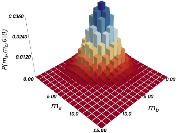
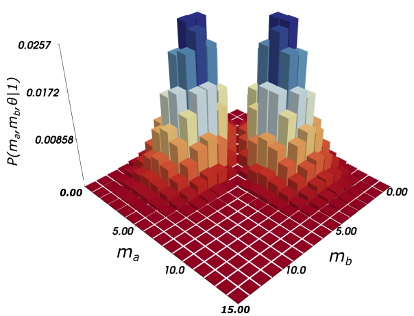
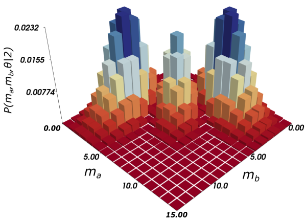
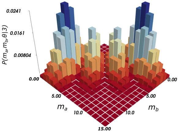
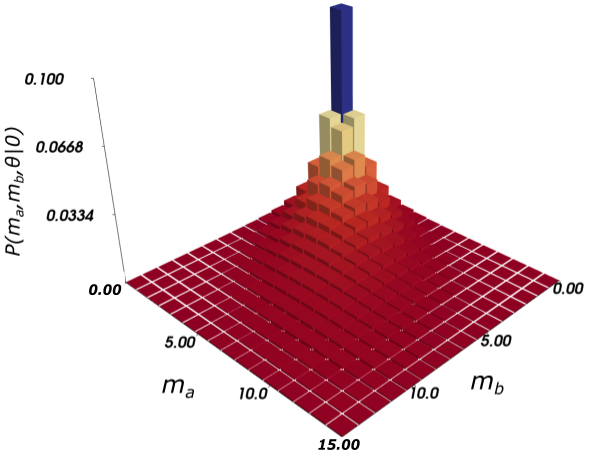
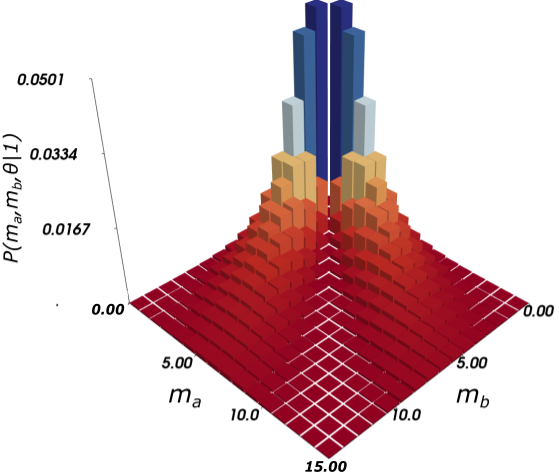
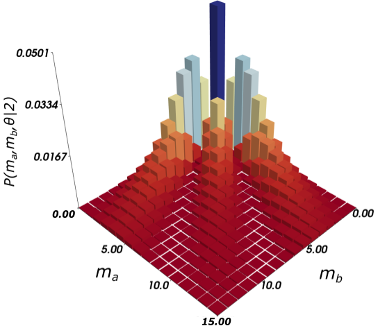
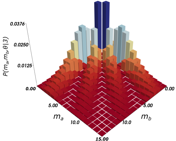
Figure 1: Joint output probability $P(m_{a},m_{b}|n)$ to measure $m_{a}$ photons in mode-1 and $m_{b}$ photons in mode-2 from a 50:50 BS for input Fock number states (FS) $|n\rangle_{1}$ in mode-1, for $n=\{0,1,2,3\}$ (top row, left to right), and an input coherent state (CS) $|\beta\rangle_{2}$ in mode-2, with mean number of photons with $\bar{n}_{2}=9$. A central nodal line (CNL) of zeros for inputs $|n,\beta\rangle_{12}$ is observed for odd $n=\{1,3\}$ indicating destructive interference of coincidence detection on all output FS/FS $|m^{\prime},m^{\prime}\rangle_{12}$. No CNL is observed for input states with even $n=\{0,2\}$ , indicating non-zero coincidence detection. (bottom row) Same as top row, but now with the CS mode-2 input state replaced by a mixed thermal state $\rho^{\textrm{thermal}}_{2}$ of average photon number $\bar{n}_{2}=9$.

The bottom row of Fig.(1) is similar to the top row, except now the input CS state is replaced by a mixed thermal state $\rho^{\textrm{thermal}}$, again of mean photon number $\bar{n}_{2}=9$, illustrating the universality of the eHOM effect.

The case of the input of a single photon and a CS $|1,\beta\rangle_{12}$ on a BS was discussed over the years by many authors, most notably Ou (of HOM fame) in 1996 Ou:1996 (and in subsequent books) Ou:2007 ; Ou_Book:2017 , and by Birrittella Mimih and Gerry BMG:2012 in 2012, but never fully explored as in eHOM_PRA:2022 (which also examined non-balanced lossless BS configurations as well). In his book “Quantum Optics for Experimentalists,” Ou_Book:2017 , Ou coins the term ”Generalized HOM effect,” (Chapter 8.3.2) in which judicious choices of the transmission coefficient (for a non-balanced lossless BS) can lead to destructive interference on chosen non-diagonal coincidence states (vs the balanced lossless BS and universality of the CNLs discussed in this work). The early work of Lai, Buz̆ek and Knight (LBK) Lai:1991 looked at the BS transformation on dual FS inputs to a fiber-coupler BS, including scattering losses (due to sidewall roughness). The work that comes closest to nearly addressing the eHOM effect was that by Campos, Saleh and Teich Campos:1989 in their extensive study of the $SU(2)$ properties of a lossless beam splitter. Once again, conditions were discussed for obtaining isolated zeros in the joint output probability distribution, for interesting special cases, but not in all generality.

In this work, we wish to consider the prospects for the experimental realization of the eHOM effect for the case of FS/CS input $|1,\beta\rangle_{12}$ to a balanced 50:50 BS. So far in the prior works of the authors eHOM_PRA:2022 ; HOMisReallyOdd:2024 the eHOM effect has been discussed in an idealized form, which has implicitly assumed that (i) the photons from both input ports arrive at the BS simultaneously, (ii) the detectors for measuring the output photons have unit efficiency, and the (iii) the photons involved are treated as monochromatic plane waves. Here we will consider the implications of these common detrimental effects likely encountered in any attempt at an experimental realization of the eHOM effect, and their degradation on the resulting destructive interference.

The outline of this paper is as follows; In Section II we briefly review the results of HOMisReallyOdd:2024 to show how the eHOM effect for FS/FS inputs $|n,m\rangle_{12}$ can be interpreted, solely diagrammatically, as a multi-photon generalization of the two-photon HOM effect. This is accomplished by keeping track of how input photons are scattered (transmitted or reflected) into output modes, and the $(-1)$ signs they encounter. In Section III we begin our examination of the prospects for an experimental realization of the eHOM effect on the $|1,1\rangle_{12}$ output coincident state, for an input consisting of a single photon FS in mode-1 and a CS (idealized laser) in mode-2. In this section we include the effects of finite (imperfect) detection efficiency. In Section IV we include the effects of the wavepacket nature of FS input photons by including spatio-temporal modes functions in our experimental examination, as well as the effect of a possible time delay between the detected output photons. For the FS/CS input, we first consider these effects on the detection of the output coincidence state $|1,1\rangle_{12}$, before examining the more involved case of detection of the general output diagonal state $|N,N\rangle_{12}$, involving photon counting theory/expressions. In Section V we present a summary and conclusion of our results.

II A diagrammatic interpretation of the extended HOM effect

Any two-port optical device such as a lossless BS is described by the unitary transformation $U$ of the input mode creation operators $a^{\dagger}_{1,in},a^{\dagger}_{2,in}$ to the output modes $a^{\dagger}_{1,out},a^{\dagger}_{2,out}$ given by

$$\hskip-36.135pt\vec{a}^{\dagger}_{out}=\left[\begin{array}[]{c}a^{\dagger}_{1,out}\\ a^{\dagger}_{2,out}\end{array}\right]=U\left[\begin{array}[]{c}a^{\dagger}_{1,in}\\ b^{\dagger}_{2,in}\end{array}\right]U^{\dagger}=\left[\begin{array}[]{cc}S_{11}&S_{12}\\ S_{21}&S_{22}\end{array}\right]\,\left[\begin{array}[]{c}a^{\dagger}_{1,in}\\ a^{\dagger}_{1,in}\end{array}\right]\equiv S\,\vec{a}^{\dagger}_{in}=\left[\begin{array}[]{c}S_{11}\,a^{\dagger}_{1,in}+S_{12}\,a^{\dagger}_{2,in}\\ S_{21}\,a^{\dagger}_{1,in}+S_{22}\,a^{\dagger}_{2,in}\end{array}\right].$$ (1)

We see that $S_{ij}$ is interpreted as the scattering of an input photon from mode-$j$ into the output mode-$i$. (Note: in the subsequent figures we have included a “backward circumflex arrow” from $j$ to $i$ to mnemonically remind the reader of the direction of the mode scattering in the amplitude $S_{ij}$). Unitarity of the $U$ requires the unitarity of $S$ which can be expressed as the requirement of the orthonormality of the columns (and rows) of $S$, yielding Skaar:2004

$$|S_{11}|^{2}+|S_{12}|^{2}=1,\quad|S_{21}|^{2}+|S_{22}|^{2}=1,\quad S_{11}\,S^{*}_{12}+S_{21}\,S^{*}_{22}=0.$$ (2)

Taking the absolute value of the last equation in Eq.(2) and using the first two equations yields $|S_{11}|=|S_{22}|$ and $|S_{12}|=|S_{21}|=\sqrt{1-|S_{11}|^{2}}$. Finally, writing each amplitude as $S_{ij}=|S_{ij}|\,e^{\theta_{ij}}$, the last equation in Eq.(2) yields the phase condition $\theta_{11}+\theta_{22}=\theta_{12}+\theta_{21}+\pi$. While there appears in the literature and textbooks many different phase conventions for a BS Loudon:2000 ; Skaar:2004 ; Agarwal:2013 ; Ou_Book:2017 ; Gerry_Knight:2023 , none of the results of the HOM or eHOM effect depends on a particular choice of phase, and so for convenience, we chose to use an anti-symmetric $2\times 2$ rotation matrix, with real entries and $S_{21}=r=-S_{12}$ eHOM_PRA:2022 . Thus, the transformation of the mode creation operators in Eq.(1) is illustrated in Fig.(2) for this phase convention, which allows us to track a single $-1$ sign change ($S_{12}$) associated with the scattering (reflection) of an input mode-2 photon off the bottom of the BS, into mode-1.

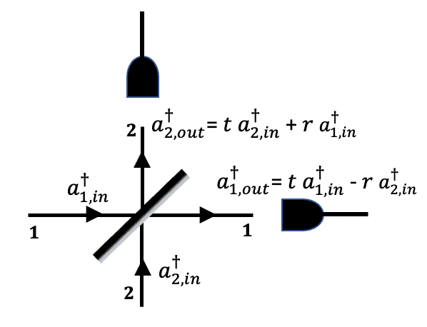
Figure 2: Output creation operators for mode-1 and mode-2 in terms of the input creation operators for a lossless beamsplitter (BS), with transmission coefficient $t$ and reflection coefficient $r$ such that $|t|^{2}+|r|^{2}\equiv T+R=1.$ In the convention employed in this work, $t$ and $r$ are taken to be real, and the $(-1)$ sign is associated with an input mode-2 photon reflecting into the output mode-1.

Again, note that in general $S_{ij}$ is defined to be Skaar:2004 the amplitude for a single photon to scatter from input mode-$j$ to output mode-$i$, as given by the rightmost BS transformation given in Eq.(1).

II.1 The Hong-Ou-Mandel effect

Before examining the eHOM effect, let us first consider the standard textbook discussion of the HOM effect Agarwal:2013 ; Ou_Book:2017 ; Gerry_Knight:2023 in terms of the scattering amplitudes of the two input photons. In Fig.(3) we consider the two-photon input state $|1,1\rangle_{12}$,

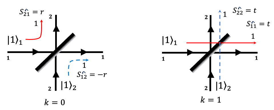
Figure 3: The 2-photon HOM effect with input $|1,1\rangle_{12}$ illustrating the two scattering amplitudes (left) $A_{k=0}$ both photons reflecting off the BS, and (right) $A_{k=1}$ both photons transmitting through the BS. Both amplitudes have equal magnitudes, yet opposite signs, that combine to create destructive interference on the coincident output state $|1,1\rangle_{12}$. In general, the integer $k\in\{0,1,\ldots,n\}$ designates the number of photons that transmit from input mode-1 to output mode-1 (with amplitude $(S_{11})^{k}$) for the FS/FS input state $|n,m\rangle_{12}$.

for the HOM effect HOM:1987 , and consider the total amplitude $A$ for coincidence on the output state $|1,1\rangle_{12}$. The total amplitude is composed of two components $A=A_{k=0}+A_{k=1}$, where, in general, $k=\{0,\ldots,n\}$ (note: without loss of generality we will only consider the cases where $n\leq m$) indicates the number of photons transmitted from input mode-1 to output mode-1 (giving rise to the contribution $(S_{11})^{k}$ in $A_{k}$). As is well known now, the HOM effect, or the complete destructive interference of the quantum amplitudes for the output on the $|1,1\rangle_{12}$, is given by the sum of the contributions where (i) both photons are reflected into opposite numbered modes by the BS, with amplitude $A_{k=0}=S_{21}\,S_{12}=(r)(-r)=-r^{2}$, and both photons transmitted into their originating numbered modes, with amplitude $A_{k=1}=S_{11}\,S_{22}=t^{2}$, as shown in Fig.(3). The crucial $(-1)$ sign in the $A_{k=0}$ amplitude comes from the contribution $(S_{12})^{1}=-r$ of the single input photon (the exponent of $S_{12}$) from mode-2 reflecting into mode-1. For a 50:50 BS where $t=r=\tfrac{1}{\sqrt{2}}$ these two amplitudes have equal magnitude, but opposite sign, and hence sum to zero: $A=A_{k=0}+A_{k=1}=(-r^{2}+t^{2})\overset{|t|=|r|}{\to}0$ (complete destructive interference) note:on:choice:of:S:in:HOM:v2 . This is the famed HOM effect HOM:1987 . Of course, this is the “textbook version” of the HOM effect, since we have implicitly assumed, that both photons (i) are completely indistinguishable (e.g. monochromatic in frequency, same spatial mode profile, etc…), (ii) have arrived at the BS at the same time (no relative time delay), and (iii) have been detected at the same time (no detection time difference). All these effects can be incorporated into the analysis of the HOM effect Legero_Rempe:2003 , and we will examine some of these considerations in later sections.

A subtle feature in Fig.(3), that is obscured by the employment of only two input photons in the HOM effect, is the $k=0$ and $k=1$ component scattering amplitudes diagrams are “mirror images” of each other. By this we mean the following. Focusing on mode-1, we see that the number of photons reflected from input mode-1 to output mode-2 (red solid arrow) for $k=0$ in Fig.(3)(left) is equal to the number of photons transmitted from input mode-1 to output mode-1(red solid arrow) for $k=1$ in Fig.(3)(right). Similarly for mode-2, the number of photons reflected from input mode-2 to output mode-1 (blue dashed arrow) for $k=0$ in Fig.(3)(left) is equal to to the number of photons transmitted from input mode-2 to output mode-2 (blue dashed arrow) for $k=1$ in Fig.(3)(right).

While this swapping of the number of photons that reflect/transmit in one diagram to number that transmit/reflect respectively in a “mirror image” diagram, but with an overall relative minus sign, may appear trivial when only two photons are involved, it actually lies at the heart of the eHOM destructive interference effect. As discussed diagrammatically in HOMisReallyOdd:2024 , for general FS/FS inputs $|n,m\rangle_{12}$ with $n$ and $m$ both odd (taking $n<m$ for concreteness, without loss of generality) there are an even number $n+1$ of component scattering amplitudes $A_{k}$, $k\in\{0,1,\ldots,n\}$ comprising the total amplitude $A=\sum_{k=0}^{n}A_{k}$, which cancel separately in pairs on the coincident output state $|\tfrac{n+m}{2},\tfrac{n+m}{2}\rangle_{12}$ via $A=\sum_{k=0}^{(n-1)/2}(A_{k}+A_{n-k})$. That is, each pair of scattering amplitudes $A_{k}+A_{n-k}$ are separately “mirror images” of each other, with equal magnitude and opposite relative minus sign when the BS is balanced (50:50), and thus cancel each other $A_{k}+A_{n-k}=0$, for $k\in\{0,1,\ldots,\tfrac{n-1}{2}\}$. Thus, one can interpret the eHOM effect as a series of HOM effects happening simultaneously on $\tfrac{n+1}{2}$ pairs of multi-photon scattering amplitudes. This can be diagrammatically shown, as in the next subsection.

Lastly, for $(n,m)$ both even there are an odd number of component scattering amplitudes, and (i) mirror image diagrams now have the same sign and therefore constructively interfere, and (ii) there is an “unpaired” non-zero scattering amplitude that is not able to cancel with any other diagram. Both these conditions imply that there cannot be destructive interference on the output coincidence state if $(n,m)$ are both even eHOM_PRA:2022 ; HOMisReallyOdd:2024 .

II.2 The extended Hong-Ou-Mandel effect

To show the pairwise cancellation of mirror image scattering amplitudes $(A_{k}+A_{k=n-k})\overset{t=r}{\to}0$ in the previous subsection for the case of a FS/FS input state $|n,m\rangle_{12}$ with $(n,m)$ both odd, consider Fig.(4) and Fig.(5) with the general odd-odd FS/FS input $|2n+1,2m+1\rangle_{12}$, with output coincident state $|n+m+1,n+m+1\rangle_{12}$.

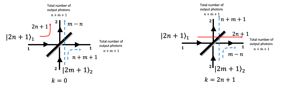
Figure 4: The odd-odd-photon eHOM effect with input state $|2n+1,2m+1\rangle_{12}$ illustrating the two “outer” scattering amplitudes $A_{k=0}$ and $A_{k=2n+1}$ (for $k\in\{0,1,\ldots,2n+1\}$), with equal magnitude and opposite signs (when $|t|=|r|$) that cancel each other, contributing to the complete destructive interference on the coincident output state $|n+m+1,n+m+1\rangle_{12}$.

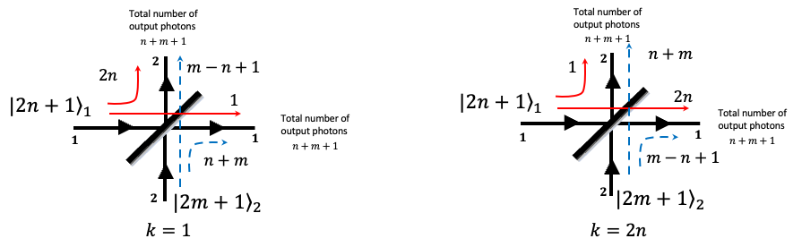
Figure 5: The odd-odd-photon eHOM effect with input $|2n+1,2m+1\rangle_{12}$ illustrating the two “penultimate outer” scattering amplitudes $A_{k=1}$ and $A_{k=2n}$ (for $k\in\{0,1,\ldots,2n+1\}$), with equal magnitude and opposite signs (when $|t|=|r|$) that cancel each other, contributing to the complete destructive interference on the coincident output state $|n+m+1,n+m+1\rangle_{12}$.

Fig.(4) considers the “outermost” pair of amplitude diagrams $A_{k=0}+A_{2n+1}$ (the minimum and maximum number of photons transmitted from input mode-1 to output mode-1, respectively), where the symmetry dictates the equality of the combinatorial factors, $C_{0}=C_{2n+1}$ HOMisReallyOdd:2024 . The amplitude for the leftmost diagram is given by $A_{k=0}=C_{0}\,(S_{11})^{0}\,(S_{21})^{2n+1}\,(S_{22})^{m-n}\,(S_{12})^{n+m+1}=C_{0}\,t^{n+m+1}\,r^{n+m+1}\,(-1)^{n+m+1}$, while the amplitude for the rightmost diagrams is given by $A_{k=2n+1}=C_{2n+1}\,(S_{11})^{2n+1}\,(S_{21})^{0}\,(S_{22})^{n+m+1}\,(S_{12})^{m-n}=C_{2n+1}\,t^{3n+m+2}\,r^{m-n}\,(-1)^{m-n}$. The sum of amplitudes for these two diagrams can be factored into the form $A_{k=0}+A_{k=2n+1}=C_{0}\,t^{n+m+1}\,r^{m-n}\,(-1)^{m-n}\,$ $[r^{2n+1}\,(-1)^{2n+1}+t^{2n+1}]\overset{|t|=|r|}{\to}0$. The crucial point of this last expression shows that while both diagrams incur multiple powers of $(-1)$ due to the scattering of mode-2 photons into mode-1 ($S_{12}$), the relative sign between the two diagrams (in the square brackets) is $(-1)^{2n+1}\equiv-1$. Thus, the pair of mirror image diagrams cancel each other for a 50:50 BS, with equal magnitude, but opposite sign.

Fig.(5) considers the “next innermost pair” of mirror image amplitude diagrams, where in a similar calculation to the above, we have $A_{k=1}+A_{k=2n}=C_{1}\,t^{m-n+2}\,r^{m-n+1}\,(-1)^{m-n+1}\,[r^{4n-2}\,(-1)^{2n-1}+t^{4n-2}]\overset{|t|=|r|}{\to}0$. Again, the symmetry of the mirror image diagrams dictates the equality of the combinatorial factors, $C_{1}=C_{2n}$. This time the relative sign between the two diagrams is $(-1)^{2n-1}\equiv-1$ (in the square brackets). Thus, once again for a 50:50 BS this pair of diagrams exhibit equal magnitudes (though different in value from that of the outermost pair) and opposite signs.

This cancellation $A_{k}+A_{2n+1-k}=0$ of mirror image scattering amplitudes for a 50:50 balanced beamsplitter occurs separately for each pair for $k\in\{0,1,\ldots,n\}$. From these observations, a simple, general analytical proof can be constructed straightforwardly, and appears in HOMisReallyOdd:2024 (see also Appendix B of eHOM_PRA:2022 for a formal, but less intuitive, proof).

III Issues for consideration for the observation of the eHOM effect with a Fock state/Coherent State input to a 50:50 BS

We now turn our attention to a consideration of experimentally realizing the eHOM effect in a laboratory setting. In a realistic experiment one has to contend with the prospects of imperfect detector efficiency, the influence of the photon mode functions in wavepackets, and potential time delay between photon detection in the output ports of the BS. In this section we consider two of these aspects in the context of a possible experimental realization of the eHOM effect for the case of a FS/CS input $|1,\beta\rangle_{12}$ with a single photon $|1\rangle_{1}$ entering port-1 of a 50:50 BS, and a coherent state $|\beta\rangle_{2}=e^{-|\beta|^{2}/2}\,\sum_{m=0}^{\infty}\tfrac{(\beta)^{m}}{\sqrt{m!}}\,|m\rangle_{2}$ of (complex) amplitude $\beta$, with mean photon number $\bar{n}_{2}=|\beta|^{2}\,$ Scully_Zubairy:1997 ; Loudon:2000 ; Agarwal:2013 ; Ou_Book:2017 ; Gerry_Knight:2023 . The coherent state represents an idealized, continuous wave (CW) laser of fixed frequency $\omega_{2}$, and has the property that it is an eigenstate of the mode-2 annihilation operator, $a_{2}\,|\beta\rangle_{2}=\beta\,|\beta\rangle_{2}$. The single photon FS could be generated for example by the heralding on one component ($1^{\prime}$) of a weak two-mode squeezed state $|TMSS\rangle_{11^{\prime}}=\frac{1}{\cosh(r)}\sum_{n=0}^{\infty}\tanh^{n}(r)|n,n\rangle_{11^{\prime}}$ where $r$ is the squeezing parameter. This state can be generated for example, by the nonlinear processes of spontaneous parametric down-conversion or by four-wave mixing Boyd:1991 ; Scully_Zubairy:1997 ; Agarwal:2013 ; Ou_Book:2017 ; Gerry_Knight:2023 ; Boyd:1991 . For a weak field TMSS, a detection in mode-$1^{\prime}$ “heralds” the correlated presence of a single photon in mode-1, which can then be fed forward into the mode-1 input port of a 50:50 BS.

III.1 Imperfect detection efficiency

The probability $P(N_{1},N_{2})$ to perfectly detect $N_{1}$ photons from mode-1 and $N_{2}$ photons from mode-2 from the output of a lossless 50:50 BS is given by $P(N_{1},N_{2})=|\mathcal{A}_{N_{1},N_{2}}|^{2}$, where the quantum amplitude is given by $\mathcal{A}_{N_{1},N_{2}}={}_{12}\langle{N_{1},N_{2}}|{1,\beta}\rangle^{out}_{12}$. For the input state $|1,\beta\rangle^{in}_{12}=a^{\dagger}_{1}\,D_{2}(\beta)|0,0\rangle_{12}$, where $D_{2}(\beta)=e^{\beta\,a^{\dagger}_{2}-\beta^{*}\,a_{2}}$ is the mode-2 displacement operator, defined such that its action on the vacuum state produces a CS, $D_{2}(\beta)|0\rangle_{2}=|\beta\rangle_{2}$ Scully_Zubairy:1997 ; Agarwal:2013 ; Ou_Book:2017 ; Gerry_Knight:2023 . The action of the BS is affected by writing the input creation operators in terms of the output creation operators (and again, dropping $in$ and $out$ subscripts for clarity) producing $|1,\beta\rangle^{out}_{12}=\frac{1}{\sqrt{2}}(a^{\dagger}_{1}+a^{\dagger}_{2})\,D_{1}(\tfrac{-\beta}{\sqrt{2}})\,D_{2}(\tfrac{\beta}{\sqrt{2}})\,|0,0\rangle_{12}=\frac{1}{\sqrt{2}}(a^{\dagger}_{1}+a^{\dagger}_{2}),|\tfrac{-\beta}{\sqrt{2}},\tfrac{\beta}{\sqrt{2}}\rangle_{12}$, where the transformation of $D_{2}(\beta)$ by the BS, and the independence of mode-1 and mode-2 operators, creates the (tensor) product of displacement of operators $D_{1}(\tfrac{-\beta}{\sqrt{2}})\,D_{2}(\tfrac{\beta}{\sqrt{2}})$, leading to a product of mode-1/mode-2 coherent states, each with reduced amplitudes $\tfrac{-\beta}{\sqrt{2}}$ and $\tfrac{\beta}{\sqrt{2}}$, respectively. Using the Hermitian conjugate of the boson operator relations that $a_{i}|N\rangle_{i}=\sqrt{N}\,|N-1\rangle_{i}$, namely ${}_{i}\langle N|\,a^{\dagger}_{i}=\sqrt{N}\,{}_{i}\langle N-1|$, it is easy to show that

$$P(N_{1},N_{2})=|{}_{12}\langle{N_{1},N_{2}}|{1,\beta}\rangle^{out}_{12}|^{2}=\frac{e^{-|\beta|^{2}}}{N_{1}!\,N_{2}!\,2^{N_{1}+N_{2}}}\,(N_{1}-N_{2})^{2},$$ (3)

which is a straightforward extension Ou:1996:Eq:4:note of a result first shown by Ou in 1996 Ou:1996 for the input state $|1,N\rangle_{12}$. The salient point here is that for $N_{1}=N_{2}$ one has a CNL of zeros along the main diagonal of the joint output probability distribution $P(N_{1},N_{2})$.

To model imperfect detection efficiency Loudon:1983 ; Scully_Zubairy:1997 ; Knight:2002 ; eHOM_PRA:2022 consider the detection of $n$ photons in the output of a single mode, with detector efficiency $0\leq\eta\leq 1$. The relevant point is that these $n$ detected photons could have resulted from $N\geq n$ photons impinging on the detector, of which only $n$ were actually registered, due the finite efficiency of the detector. The the probability that $n$ photons were detected, which $N-n$ were not, is the Bernoulli factor $\binom{N}{n}\,\eta^{n}\,(1-\eta)^{N-n}$, where the binomial coefficient indicates the indistinguishability of which $n$ of the total of the impinging $N$ photons were actually detected. The total probability $P_{\eta}(n)$ is then a sum over all possible values of $N\geq n$, namely $P_{\eta}(n)=\sum_{N=n}^{\infty}\binom{N}{n}\,\eta^{n}\,(1-\eta)^{N-n}\,P_{N}$ , where $P_{N}=|\mathcal{A}_{N}|^{2}$ is the probability to perfectly detect $N$ photons quantum:efficiency:note . Applying this to each output mode of the BS, and assuming equal detector efficiencies, the joint probability $P_{\eta}(n,n)$ to measure $n$ coincidence counts from the output of the BS for the input $|1,\beta\rangle_{12}$ is given by

$$P_{\eta}(n,n) = \sum_{N_{1}=n}^{\infty}\,\sum_{N_{2}=n}^{\infty}\,\binom{N_{1}}{n}\,\binom{N_{2}}{n}\,\eta^{2\,n}\,(1-\eta)^{N_{1}+N_{2}-2n}\,P(N_{1},N_{2}),$$ (4)

$$= 2\,\eta^{2\,n}\sum_{N_{1}>N_{2}\geq n}^{\infty}\,\binom{N_{1}}{n}\,\binom{N_{2}}{n}\,\eta^{2\,n}\,(1-\eta)^{N_{1}+N_{2}-2n}\,P(N_{1},N_{2})>0.$$

In the last line of Eq.(4) we have broken the double sum into two pieces: (i) a single diagonal sum over $N_{1}=N_{2}$, which is zero, since $P(N_{1},N_{1})=0$ by Eq.(3), and (ii) the remaining off-diagonal double sum, now with $N_{1}>N_{2}\geq n$, with a factor of $2$ out front (due to the symmetry of the entire expression under the exchange $N_{1}\leftrightarrow N_{2}$). Thus, while the presence of the CNL can be observed, it is no longer exactly zero. In addition, detecting the coincidence output state $|n,n\rangle_{12}$ is proportional to $\eta^{2\,n}\ll 1$ at very high $n$. Thus, the prospects for detecting the presence of the CNL is best for very low photon number (e.g. $n\in\{1,2\}$, and suggests the use of photon number resolving detectors, as suggested in eHOM_PRA:2022 , which can now detect and number-resolve up to 100 individual photons eaton_pfister_100_photons:2023 .

IV Space-time domain considerations

In the previous sections, we have modeled the FS/FS inputs $|n,m\rangle_{12}$ as idealized monochromatic, single frequency entities, with (i) photons from both input ports arriving at the BS simultaneously (no time delay between input photons), and similary (ii) photons detected in the output ports simultaneously (no detection time difference). Such effects can be included by considering the photons as arriving in wavepackets, with a finite frequency spread about a central frequency, and incorporating detection delay times. A general analysis in the frequency domain for an $N$-photon FS $|N\rangle$, with possible arbitrary $k$ sub-groupings of the photons into time-distinguishable groups containing $N_{k}$ photons such that $\sum_{k}N_{k}=N$, was carried out by Ou Ou:1996 ; Ou:2007 ; Ou_Book:2017 . However, for our purposes, it is sufficient to consider all photons in both input modes, to each be in their own single spatio-temporal mode (and hence indistinguishable). We can include the effects of time delays $\delta\tau$ between the input wavepackets of mode-1 and mode-2, and a difference $\tau$ in the detection time of the output mode-1 and mode-2 photons, as described in Legero et al. Legero_Rempe:2003 . While this analysis can be carried out in either the frequency or the space-time domain, the authors Legero_Rempe:2003 advocated that there is less computation involved when using the time domain, as we shall also use here. Lastly, for simplicity, in this section we will assume unit detection efficiency. The effects of finite detection efficiency can be straightforwardly included afterwards using the Bernoulli trial analysis of the previous section.

The main idea Legero_Rempe:2003 is that one assumes the Hilbert space of states is spanned by an orthonormal set of spatio-temporal modes $\zeta_{k}(t)$ such that the positive and negative electric field operators $E^{+}(t)$ and $E^{-}(t)$ (with total electric field $E(t)=E^{+}(t)+E^{-}(t)$) are given by $E^{+}(t)=\sum_{k}\zeta_{k}\,a_{k}$ and $E^{-}(t)=\sum_{k}\zeta_{k}\,a^{\dagger}_{k}$. Then, all that has to be modified from Eq.(1) for a 50:50 BS is

$$\hskip-36.135pt\left[\begin{array}[]{c}E^{+}_{1,out}\\ E^{+}_{2,out}\end{array}\right]=\frac{1}{\sqrt{2}}\,\left[\begin{array}[]{c}E^{+}_{1,in}-E^{+}_{2,in}\\ E^{+}_{2,in}+E^{+}_{1,in}\end{array}\right]=\frac{1}{\sqrt{2}}\,\left[\begin{array}[]{c}\zeta_{1}(t)\,a_{1,in}-\zeta_{2}(t)\,a_{2,in}\\ \zeta_{2}(t)\,a_{2,in}+\zeta_{1}(t)\,a_{1,in}\end{array}\right].$$ (5)

IV.1 Space-time analysis of the HOM effect: A brief summary of Legero et al. Legero_Rempe:2003

Consider the two-photon HOM input state $|\Psi_{in}\rangle_{12}=|1,1\rangle_{12}=a^{\dagger}_{1,in}\,a^{\dagger}_{2,in}\,|0,0\rangle_{12}$. The from Glauber’s detection theory Loudon:1983 ; Loudon:2000 , the joint probability $P_{1_{1},1_{2}}(t_{0},\tau)$ to detect an output photon in mode-1 at (arbitrary) time $t_{0}$, and the output photon in mode-2 at time $t_{0}+\tau$ is given by $P_{1_{1},1_{2}}(t_{0},\tau)=|\langle{\Psi_{out}}|{\Psi_{out}}\rangle|^{2}$ where $|\Psi_{out}\rangle_{12}=E^{+}_{2,out}\,E^{+}_{1,out}|\Psi_{in}\rangle_{12}$ using Eq.(5), which annihilates the two photons at two different times, separated by the time difference $\tau$. Using the boson operator identity for any mode-$i$, $a_{i}\,a^{\dagger}_{i}\equiv[a_{i},a^{\dagger}_{i}]+a^{\dagger}_{i}\,a_{i}=1+a^{\dagger}_{i}\,a_{i}$ and $a_{i}|0\rangle_{i}=0$, and the independence of mode-1 and mode-2, one can push the creation operators in $|\Psi_{in}\rangle_{12}$ to the left of the annihilation operators in electric field operators $E^{+}_{2,out}\,E^{+}_{1,out}$ (i.e. arranging the operators in normal order), to see that only the commutators $[a_{i},a^{\dagger}_{i}]|00\rangle_{12}=|00\rangle_{12}$ contribute to $|\Psi_{out}\rangle_{12}$ (since in normal order the annihilation operators will annihilate the vacuum state). A straightforward calculation produces $\langle{\Psi_{out}}|{\Psi_{out}}\rangle=\frac{1}{2}\big{(}\zeta_{1}(t_{0}+\tau)\,\zeta_{2}(t_{0})-\zeta_{2}(t_{0}+\tau)\,\zeta_{1}(t_{0})\big{)}$ for a joint output probability given by Legero et al. Legero_Rempe:2003

$$P^{(HOM)}_{1_{1},1_{2}}(t_{0},\tau)=\tfrac{1}{4}\,|\zeta_{1}(t_{0}+\tau)\,\zeta_{2}(t_{0})-\zeta_{2}(t_{0}+\tau)\,\zeta_{1}(t_{0})|^{2}.$$ (6)

As pointed out by the authors, if the photons are detected simultaneously ($\tau=0$), then $P^{(HOM)}_{1_{1},1_{2}}=0$ regardless of the form of the spatio-temporal mode functions.

The above assumes the detection time difference $\tau$ is much smaller than the mutual coherence time $\tau_{c}$ of the incoming photons. If this is not the case, then the interference terms in Eq.(6) washes out when averaged over an ensemble of different photon pairs and one has $P^{(HOM)}_{1_{1},1_{2}}(t_{0},\tau)\overset{\tau\gg\tau_{c}}{\longrightarrow}\tfrac{1}{4}\,\big{(}P_{1}(t_{0}+\tau)\,P_{2}(t_{0})+P_{2}(t_{0}+\tau)\,P_{1}(t_{0})\big{)}$ where $P_{i}(t)={}_{12}\langle\Psi_{in}|E^{-}(t)\,E^{+}(t)|\Psi_{in}\rangle$ is the probability (proportional to the intensity) to measure the photon in output port-$i$.

To study quantum beating between the two-photons in the HOM effect, Legero et al. Legero_Rempe:2003 used the normalized spatio-temporal Gaussian mode functions ($\int_{-\infty}^{\infty}|\zeta_{i}(t)|^{2}\,dt=1$)

$$\zeta_{1} = \sqrt[4]{2/\pi}\;e^{-(t-\delta\tau/2)^{2}-i\,(\omega-\Delta\omega/2)t},$$ (7a)

$$\zeta_{2} = \sqrt[4]{2/\pi}\;e^{-(t+\delta\tau/2)^{2}-i\,(\omega+\Delta\omega/2)t},$$ (7b)

where $\omega=\frac{1}{2}\,({\omega}_{1}+{\omega}_{2})$ and $\Delta{\omega}=({\omega}_{1}-{\omega}_{2})$ are the average and difference between the two mode-1 and mode-2 frequencies ${\omega}_{1}$ and ${\omega}_{2}$, respectively. Here, $\delta\tau$ is the total time delay between the center frequencies of the mode-1 and mode-2 input wavepackets. The total probability is obtained by integrating over all possible values of the arbitrary detection time $t_{0}$ of the first photon and is given by Legero_Rempe:2003

$$\hskip-14.45377ptP^{(HOM)}_{1_{1},1_{2}}(\tau,\delta\tau,\Delta{\omega})=\int\,dt_{0}\,P^{(HOM)}_{1_{1},1_{2}}(t_{0},\tau,\delta\tau,\Delta{\omega})=\frac{\cosh(2\tau\,\delta\tau)-\cos(\Delta{\omega}\,\tau)}{2\,\sqrt{\pi}}\;e^{-(\tau^{2}+\delta\tau^{2})}.$$ (8)

Other realistic experimental effects can be incorporated such as (i) inhomogeneous broadening of the frequency difference (using a normalized Gaussian distribution $f_{\delta{\omega}}(\Delta{\omega})=\tfrac{1}{\delta{\omega}\,\sqrt{\pi}}\,e^{-(\Delta{\omega}/\delta{\omega})^{2}}$), and (ii) integrating over the detection time difference $\tau$ to obtain

$$\hskip-14.45377ptP^{(HOM)}_{\textrm{total};1_{1},1_{2}}(\delta\tau,\delta{\omega})=\int\int\,d\tau\,d\Delta{\omega}\,f_{\delta{\omega}}(\Delta{\omega})\,P^{(HOM)}_{1_{1},1_{2}}(\tau,\delta\tau,\Delta{\omega})=\frac{1}{2}-\frac{e^{-\delta\tau^{2}}}{\sqrt{4+\delta{\omega}^{2}}}\overset{\delta\tau\gg\sigma_{t}}{\longrightarrow}\frac{1}{2}.$$ (9)

Eq.(9) shows that the HOM effect vanishes if the two wavepackets are delayed in time by greater than the width of their wavepackets $\sigma_{t}$, since they are then distinguishable photons.

IV.2 Space-time analysis of the Fock state/coherent state input state $|1,\beta\rangle_{12}$

In this section we once again analyze the FS/CS input state $|1,\beta\rangle_{12}$, and the possibility to observe the eHOM effect on the output coincidence state $|1,1\rangle_{12}$, but now from a space-time analysis, as in the previous section. We take as our spatio-temporal mode functions

$$\zeta_{1}(t)=\sqrt[4]{\frac{2}{\pi\,\tau^{2}_{c}}}\;e^{-i\,{\omega}_{1}\,t-t^{2}/\tau^{2}_{c}},\qquad\zeta_{2}(t)=\sqrt{\mathcal{F}}\,e^{-i\,{\omega}_{2}\,t}\,e^{i\,\theta}.$$ (10)

In the above, we have modeled the CW laser as a single frequency exponential of frequency ${\omega}_{2}$ with phase $\theta$, following Loudon Loudon:2000 . Here, $\mathcal{F}$ is the laser flux such that in frequency space $f({\omega})=\mathcal{F}\,\delta({\omega}-{\omega}_{2})$ and $\langle{a^{\dagger}_{2}\,a_{2}}\rangle_{12}=\int d{\omega}\,f({\omega})=\mathcal{F}=\int dt\,f(t)$. For the single mode-1 input wavepacket, we have taken a normalized Gaussian of FWHM  $\tau_{c}=1/\Delta{\omega}$ where $\Delta{\omega}$ is the frequency bandwidth of the mode-1 wavepacket with center frequency ${\omega}_{1}$.

Since the mode-2 input is an idealized CW laser, there is no time delay $\delta\tau$ between mode-1 and mode-2 - i.e. the monochromatic laser is technically an infinite width pulse in time. If we instead wanted to consider a laser pulse, we could use a similar normalized Gaussian mode function for mode-2 as in Eq.(10) with temporal width $\tau_{2,c}$, and consider $\tau_{2,c}\gg\tau_{1,c}$ so that the mode-1 wavepacket is always “under” the mode-2 laser “wavepacket.” To keep things simple, we instead use the mode functions in Eq.(10), effectively taking $\tau_{2,c}\to\infty$ and writing $\tau_{1,c}\to\tau_{c}$. The analysis then proceeds in a similar fashion to the HOM case considered previously, but now for the FS/CS input state $|\Psi_{in}\rangle_{12}=|1,\beta\rangle_{12}=a^{\dagger}_{1,in}\,|0,\beta\rangle_{12}$.

We then form (upon dropping the $in$ subscripts on the operators),

$$|\Psi_{out}\rangle_{12} = E_{2,out}^{+}(t_{0}+\tau)\,E_{1,out}^{+}(t_{0})\,a^{\dagger}_{1,in}\,|0,\beta\rangle_{12}$$ (11)

$$= \frac{1}{2}\Big{[}\zeta_{1}(t_{0}+\tau)\zeta_{1}(t_{0})\,a^{2}_{1}-\zeta_{2}(t_{0}+\tau)\zeta_{2}(t_{0})\,a^{2}_{2}$$

$$- \big{(}\zeta_{1}(t_{0}+\tau)\zeta_{2}(t_{0})-\zeta_{2}(t_{0}+\tau)\zeta_{1}(t_{0})\big{)}\,a_{1}\,a_{2}\Big{]}\,a^{\dagger}_{1}\,|0,\beta\rangle_{12},$$

$$= -\frac{1}{2}\,\Big{[}\zeta_{2}(t_{0}+\tau)\zeta_{2}(t_{0})\,\beta^{2}a^{\dagger}_{1}+(\zeta_{1}(t_{0}+\tau)\zeta_{2}(t_{0})-\zeta_{2}(t_{0}+\tau)\zeta_{1}(t_{0}))\,\beta\Big{]}\,|0,\beta\rangle_{12},\qquad$$

where the term linear in $\beta$ is the same interference amplitude that appeared in the HOM calculation in Section IV.2. In going from the second to the third equality, we have used the fact that $a^{2}_{1}\,a^{\dagger}_{1}\equiv[a^{2}_{1},a^{\dagger}_{1}]+a^{\dagger}_{1}\,a^{2}_{1}=2\,a_{1}+a^{\dagger}_{1}\,a^{2}_{1}$, with both terms acting to the right, annihilating the mode-1 vacuum $|0\rangle_{1}$. When forming $P_{1_{1},1_{2}}(t_{0},\tau)=|\langle{\Psi_{out}}|{\Psi_{out}}\rangle|^{2}$ only “like” powers of $(a^{\dagger}_{1})^{k}$ for $k\in\{0,1\}$ contributed to the final result (again using $a_{1}\,a^{\dagger}_{1}=1+a^{\dagger}_{1}\,a_{1})$, since all other terms involve lone operators $a_{1}$ or $a^{\dagger}_{1}$ which annihilate the mode-1 vacuum when acting to the right or left, respectively. Thus, we obtain

$$P^{|1,\beta\rangle_{12}}_{1_{1},1_{2}}(t_{0},\tau) = \frac{1}{4}\left(P^{2}_{2}(t_{0})\,\bar{n}_{2}^{2}+|\zeta_{1}(t_{0}+\tau)\zeta_{2}(t_{0})-\zeta_{2}(t_{0}+\tau)\zeta_{1}(t_{0})|^{2}\,\bar{n}_{2}\right),$$ (12a)

$$=\frac{1}{4}\,F\,\bar{n}_{2}^{2} + 2\,F\,\bar{n}_{2}\,\sqrt{\frac{2}{\pi\,\tau^{2}_{c}}}\,e^{-\tau^{2}/2\,\tau^{2}_{c}}\,e^{-2\,(t_{0}+\tau/2)^{2}/2\,\tau^{2}_{c}}\,\Big{(}\cosh(\tau(2\,t_{0}+\tau)/\tau^{2}_{c})-\cos(\Delta{\omega}\,\tau)\Big{)},\qquad\;\;$$ (12b)

where $\Delta{\omega}\overset{\textrm{def}}{=}{\omega}_{1}-{\omega}_{2}$ and $P_{2}(t_{0})=P_{2}(t_{0}+\tau)$ is the probability to detect a photon from the mode-2 input CS $|\beta\rangle_{2}$, with mean number of photons $\bar{n}_{2}=|\beta|^{2}$. The first non-interfering, DC term in Eq.(12a) arises from the squared amplitude for the process in which both of the output photons in the two-photon coincidence detection come from the CS. The second, interference term, is the probability that the output coincidence pair consists of one photon from each mode. The origin of this term is somewhat obscured by the use of a CS, which is an eigenstate of the mode-2 annihilation operator, $a_{2}|\beta\rangle_{2}=\beta\,|\beta\rangle_{2}$. A calculation similar to Eq.(11), but now with input state $|n,m\rangle_{12}$, produces three amplitudes $|\Psi_{out}\rangle_{12}^{|n,m\rangle_{12}}=\mathcal{A}_{1}+\mathcal{A}_{2}+\mathcal{A}_{3}$ with (i) $\mathcal{A}_{1}=\tfrac{1}{4}\,\big{(}\zeta_{1}(t_{0}+\tau)\,\zeta_{1}(t_{0})\,\sqrt{n(n-1)}\big{)}$, the DC amplitude for both of the output coincidence photons to come from mode-1, (ii) $\mathcal{A}_{2}=\tfrac{1}{4}\,\big{(}\zeta_{2}(t_{0}+\tau)\,\zeta_{2}(t_{0})\,\sqrt{m(m-1)}\big{)}$, the DC amplitude for both of the output coincidence photons to come from mode-2, and finally (iii) $\mathcal{A}_{3}=-\tfrac{1}{4}\,\big{(}\zeta_{1}(t_{0}~+~\tau)\,\zeta_{2}(t_{0})-\zeta_{2}(t_{0}~+~\tau)\,\zeta_{1}(t_{0})\big{)}\,\sqrt{n\,m}$, the HOM interference amplitude for the output coincidence pair to consist of one photon from mode-1 and the other photon from mode-2.

Coming back to the calculation yielding Eq.(12a) with input state $|1,\beta\rangle_{12}$, note that the first DC term in Eq.(12a) is multiplied by $(\bar{n}_{2})^{2}$, since this term arises from both of the detected photons coming from the CS, while the second, eHOM interference term is multiplied by only $\bar{n}_{2}$, since then only one photon comes from the CS. Thus, in order to observe the eHOM effect on the coincidence output state $|1,1\rangle_{12}$, one would have to measure the first term $\tfrac{1}{4}P^{2}_{2}(t_{0})\,\bar{n}_{2}^{2}$ from the input mode-2 CS alone (from direct photon counting measurements), and subtract this off from $P^{|1,\beta\rangle_{12}}_{1_{1},1_{2}}(t_{0},\tau)$ in Eq.(12a) in order to observe the HOM-like interference term proportional to $\bar{n}_{2}$. The total probability for detecting one photon in each of output ports 1 and 2 with a time difference of $\tau$ is given by integrating the HOM interference term in Eq.(12b) over all (arbitrary) values of $t_{0}$, which yields

$$P^{|1,\beta\rangle_{12}}_{1_{1},1_{2}}(\tau)=\frac{1}{4}\,F\,\bar{n}_{2}^{2}+\frac{1}{2}\,F\,\bar{n}_{2}\left(1-e^{-\tau^{2}/2\,\tau^{2}_{c}}\,\cos(\Delta{\omega}\,\tau)\right).$$ (13)

Again, for $\tau=0$ the HOM-like interference term in Eq.(13) is zero, regardless of the frequency difference $\Delta{\omega}$. In the other extreme, the second term in Eq.(13) reduces to $\frac{1}{2}\,F\,\bar{n}_{2}$ if the second term in the parentheses either (i) vanishes when $\tau\gg\tau_{c}$, even if $\Delta{\omega}=0$ (identical frequencies), or (ii) washes out if $\tau\gg 1/\Delta{\omega}$. Thus, the prospects for observing the eHOM effect on the coincidence output state $|1,1\rangle_{12}$ for the FS/CS input state $|1,\beta\rangle_{12}$ is optimal for indistinguishable photons detected simultaneously.

IV.3 Higher Order Multi-photon Counting

In this last section we provide an indication of how higher order multi-photon counting is computed using the classic quantum photon counting formula developed by Kelly and Kleiner Kelly_Kleiner:1964 ; Loudon:1983 ; Ou:1996 . This formula would be necessary for example, for measuring the output coincident state $|N,N\rangle_{12}$ for the FS/CS input state $|1,\beta\rangle_{12}$, considered in the last section, for $N>1$. For a two-port device one, has for the probability to detect $N_{1}$ photons in mode-1, and $N_{2}$ photons in mode-2, with detector efficiencies $\eta_{1}$ and $\eta_{2}$, respectivelyOu:1996 , is given by

$$\hskip-46.97505ptP_{\eta_{1},\eta_{2}}(N_{1},N_{2})=\textrm{Tr}\left[\rho_{12}\,:\tfrac{\left(\eta_{1}\,a^{\dagger}_{1,out}\,a_{1,out}\right)^{N_{1}}\,e^{-(\eta_{1}\,a^{\dagger}_{1,out}\,a_{1,out})}}{N_{1}!}\,\tfrac{\left(\eta_{2}\,a_{2,out}\,a^{\dagger}_{2,out}\right)^{N_{2}}\,e^{-(\eta_{2}\,a^{\dagger}_{2,out}\,a_{2,out})}}{N_{2}!}:\right],$$ (14)

where $\rho_{12}$ is a general bipartite density matrix (we’ve been considering the pure cases when $\rho_{12}~=~|\Psi_{in}\rangle_{12}\langle\Psi_{in}|$). In Eq.(14) the double colons $:O(a,a^{\dagger}):$ are the conventional notation for putting the operator $O(a,a^{\dagger})$ in normal order, defined by simply reordering any operator expression by placing all the creation operators to the left, and all annihilation operators to the right, without regard for the boson commutation relations. As an example, whereas $(a^{\dagger}\,a)^{2}\equiv a^{\dagger}(a\,a^{\dagger})\,a=a^{\dagger}([a,a^{\dagger}]+a^{\dagger}\,a)\,a=(a^{\dagger})^{2}\,a^{2}+a^{\dagger}\,a$, for normal ordering we simply have $:(a^{\dagger}\,a)^{2}:~\overset{\textrm{def}}{=}~(a^{\dagger})^{2}\,a^{2}$ directly, by reshuffling (normal ordering) the operators. The process of normal ordering is appropriate for physical detectors, since in expressions such as ${}_{in}\langle{(a^{\dagger})^{2}\,a^{2}}\rangle_{in}$, the annihilation operators (acting to the right) only remove photons from the input state $a^{2}|\Psi_{in}\rangle$ (as opposed to creating photons in the detector), and the term $\langle\Psi_{in}|(a^{\dagger})^{2}$ is the corresponding Hermitian conjugate of the previous term, which (acting to the left, only) removes photons from $\langle\Psi_{in}|$.

For a 50:50 BS (i) the output creation and annihilation operators in Eq.(14) are replaced by their expressions in terms of the input operators, as in Eq.(5), (with or without the spatio-temporal mode functions), (ii) the powers and exponentials of operators are expanded in terms of (binomial) series, and finally (iii) all operators in this complicated expression are normally ordered.

IV.3.1 A single mode example

To illustrate the above procedure, consider (for simplicity) just the single mode-1, and no BS, i.e. let $a_{1,out}\to a$ and $\rho_{12}\to\rho$ and $\eta_{1}\to\eta$ (this is just a detector placed in front of the input mode-1 state). Taking the trace in Eq.(14) over FS $|N\rangle$, we have schematically $\textrm{Tr}[\rho:O(a^{\dagger}\,a):]$ where $O(a^{\dagger}\,a)$ is a function of the number operator and hence diagonal in the number basis. Therefore, $\textrm{Tr}[\rho:O(a^{\dagger}\,a):]=\sum_{N}P_{N}\left(:O(a^{\dagger}\,a):\right)_{N}$ where $P_{N}\overset{\textrm{def}}{=}\langle N|\rho|N\rangle$ and $\left(:O(a^{\dagger}\,a):\right)_{N}\overset{\textrm{def}}{=}$ $\langle N|:O(a^{\dagger}\,a):|N\rangle$. Thus, the single mode version of Eq.(14) is Loudon:1983

$$P_{\eta}(n) = \sum_{N}\,P_{N}\langle N|:\,\frac{(\eta\,a^{\dagger}\,a)^{n}}{n!}\,\sum_{k=0}^{\infty}\frac{(-\eta\,a^{\dagger}\,a)^{k}}{k!}\,:|N\rangle,$$ (15)

$$= \sum_{N}\,P_{N}\,\frac{\eta^{n}}{n!}\,\sum_{k=0}^{\infty}\frac{(-\eta)^{k}}{k!}\,\langle N|(a^{\dagger})^{n+k}\,a^{n+k}|N\rangle,$$

$$= \sum_{N}P_{N}\,\frac{\eta^{n}}{n!}\,\sum_{k=0}^{\infty}\frac{(-\eta)^{k}}{k!}\,\frac{N!}{(N-(n+k))!},$$

$$\equiv \sum_{N=n}^{\infty}P_{N}\,\eta^{N}\,\frac{N!}{n!(N-n)!}\,\sum_{k=0}^{N-n}\frac{(N-n)!}{k!(N-(n+k))!}\,(1)^{(N-(n-k))}(-\eta)^{k}$$

$$= \sum_{N=n}^{\infty}P_{N}\binom{N}{n}\eta^{n}\,(1-\eta)^{N-n},$$

where in the second line we have normally ordered the operators before taking the expectation value with respect to the FS $|N\rangle$. In the third line we have used $a^{n+k}|N\rangle=\sqrt{\tfrac{N!}{(N-(n+k))!}}\,|N-(n+k)\rangle$, and in the penultimate line we have multiplied and divided by $(N-n)!$, and have used the binomial expansion of $(1-\eta)^{N-n}$ to form the last line. Eq.(15) is the single mode version of Eq.(4). A straightforward calculation reveals that the mean number $\bar{n}$ of photons registered by the detector is given by $\bar{n}\overset{\textrm{def}}{=}\sum_{n}n\,P_{\eta}(n)=\eta\,\bar{N}$, where $\bar{N}\overset{\textrm{def}}{=}\sum_{N}N\,P_{N}$ is the mean number of photons from the input source (as measured by an idealized, unit efficiency detector).

When a BS is involved the $out$ operators in Eq.(14) must be replaced by their expressions in terms of the $in$ operators per Eq.(5) (with or without the mode functions). With $\eta_{1}=\eta_{2}\overset{\textrm{def}}{=}\eta$, the normal ordered expression of the operators in Eq.(14) is given by

$$\frac{\eta^{N_{1}+N_{2}}}{N_{1}!\,N_{2}!}\,\sum_{k=0}^{\infty}\sum_{\l=0}^{\infty}\,\frac{(-\eta)^{k+\l}}{k!\,\l!}\,(a_{1,out}^{\dagger})^{N_{1}+k}\,(a_{2,out}^{\dagger})^{N_{2}+\l}\,(a_{1,out})^{N_{1}+k}\,(a_{2,out})^{N_{2}+\l}\,$$ (16)

leading to the joint output probability

$$P_{\eta}(N_{1},N_{2}) = \frac{\eta^{N_{1}+N_{2}}}{N_{1}!\,N_{2}!}\,\sum_{k=0}^{\infty}\sum_{\l=0}^{\infty}\,\frac{(-\eta)^{k+\l}}{k!\,\l!}\,{}_{12}\langle{\Psi^{k\l}_{out}}|{\Psi^{k\l}_{out}}\rangle_{12},$$ (17a)

$$|\Psi^{k\l}_{out}\rangle_{12} \overset{\textrm{def}}{=} (a_{1,out})^{N_{1}+k}\,(a_{2,out})^{N_{2}+\l}\,|\Psi_{in}\rangle_{12},$$ (17b)

$$= \frac{1}{\sqrt{2^{N_{1}+N_{2}+k+\l}}}\,\sum_{r=0}^{N_{1}+k}\sum_{s=0}^{N_{2}+\l}\,\binom{N_{1}+k}{r}\,\binom{N_{2}+\l}{r}(-1)^{N_{1}+k-r}\,$$

$$\times \zeta^{r}_{1}(t_{0})\,\zeta^{s}_{1}(t_{0}+\tau)\,\zeta^{N_{1}+k-r}_{2}(t_{0})\,\zeta^{N_{2}+\l-s}_{2}(t_{0}+\tau)\,a_{1}^{r+s}\,a_{2}^{N_{1}+N_{2}+k+\l-(r+s)}\,|\Psi_{in}\rangle_{12},\quad\qquad$$

where we have dropped the $in$ subscript on the annihilation operators after employing Eq.(5).

IV.3.2 Balanced beamsplitter with $|1,\beta\rangle_{12}$ input state

If we now consider the input state $|\Psi_{in}\rangle_{12}=|1,\beta\rangle_{12}$ with one photon in mode 1, we see that there are only two sets of contributions in the amplitude sums $a_{1}^{r+s}\,|1\rangle_{1}$ in Eq.(17b), namely $(r,s)_{1}=(0,0)$ and $(r,s)_{2}\in\{(0,1),(1,0)\}$. The first term $(r,s)_{1}=(0,0)$ yields a DC contribution $P^{(1)}_{\eta}(N_{1},N_{2})$ to the joint output probability $P_{\eta}\overset{\textrm{def}}{=}P^{(1)}_{\eta}+P^{(2)}_{\eta}$ given by

$$P^{(1)}_{\eta}(N_{1},N_{2})=\frac{p^{N_{1}}\,e^{-p}}{N_{1}!}\,\frac{p^{N_{2}}\,e^{-p}}{N_{2}!}\,P^{2}_{2}(t_{0})\,\bar{n}_{2},\qquad p\overset{\textrm{def}}{=}\frac{1}{2}\,\eta\,\bar{n}_{2}\,P_{2}(t_{0}),$$ (18)

where we have used $P_{2}(t_{0})=|\zeta_{2}(t_{0})|^{2}=P_{2}(t_{0}+\tau)$ for the CS $|\beta\rangle_{2}$, using Eq.(10). For this contribution all the detected photons come from the CS since $(r,s)_{1}=(0,0)$ indicates that no mode-1 photons are annihilated by the detector, and the resulting state in the amplitude Eq.(17b) is proportional to $|1,\beta\rangle_{12}$,

The second set of amplitude contributions in Eq.(17b) arises from the pair $(r,s)_{2}\in\{(0,1),(1,0)\}$, and yields a state proportional to $|0,\beta\rangle_{12}$. Here, the mode-1 photon is annihilated along with mode-2 photons, allowing for the possibility of interference. The two amplitude contributions have a relative minus sign due to the factor $(-1)^{r}=\{1,-1\}$ for $r=\pm 1$ in Eq.(17b) for the two terms. The total joint probability is then given by

$$P_{\eta}(N_{1},N_{2}) = \frac{\eta^{2}\,\bar{n}_{2}}{4N_{1}N_{2}}\frac{p^{N_{1}-1}}{(N_{1}-1)!}\,\frac{p^{N_{2}-1}}{(N_{2}-1)!}\,\sum_{k=0}^{\infty}\,\sum_{\l=0}^{\infty}\,\frac{(-p)^{k}}{k!}\,\frac{(-p)^{\l}}{\l!}\,$$

$$\times \left[P_{2}(t_{0})\,P_{2}(t_{0}+\tau)\,\bar{n}_{2}+\left|(N_{2}+\l)\,\zeta_{1}(t_{0}+\tau)\,\zeta_{2}(t_{0})-(N_{1}+k)\,\zeta_{1}(t_{0})\,\zeta_{2}(t_{0}+\tau)\right|^{2}\right],\qquad$$

$$\overset{\textrm{def}}{=} P^{(1)}_{\eta}(N_{1},N_{2})+P^{(2)}_{\eta}(N_{1},N_{2}).$$

The interference term appears as the second term in the large square parentheses in Eq.(IV.3.2), which is readily apparent when we set $N_{1}=N_{2}=N$ to examine the diagonal of the joint output probability. The second term in the square brackets becomes $\left|N\mathcal{A}+\l\,\zeta_{1}(t_{0}+\tau)\,\zeta_{2}(t_{0})-k\,\zeta_{1}(t_{0})\,\zeta_{2}(t_{0}+\tau)\right|^{2}$ with $\mathcal{A}=\zeta_{1}(t_{0}+\tau)\,\zeta_{2}(t_{0})-\zeta_{1}(t_{0})\,\zeta_{2}(t_{0}+\tau)$ the HOM interference amplitude from the previous sections.

The somewhat involved expression for $P_{\eta}(N_{1},N_{2})$ in Eq.(IV.3.2) arises from the fact that we are asking for the interference from an input state $|1,\beta\rangle_{12}$ with only a single photon in mode-$1$, yet we are observing $N_{1}$ photons in the output of mode-$1$. Thus, $N_{1}-1$ photons in the observed output mode-$1$ must be coming from the input CS in mode-$2$. The interference term in Eq.(IV.3.2) describes all the possible ways that the single mode-$1$ input photon can interfere with each of the $N_{1}-1$ CS mode-$2$ input photons.

To make connection to the idealized eHOM effect in Section II (and in eHOM_PRA:2022 ), we set $\tau=0$, which in all practical purposes is experimentally realizable to within a full width half maximum set by the “jitter time” $\tau_{\textrm{jitter}}$ of the detector, i.e. $\tau\geq\tau_{\textrm{jitter}}$, where $\tau_{\textrm{jitter}}$ can be as low as $\sim 15-25\textrm{ps}$ for some detectors. Since $\mathcal{A}\overset{\tau\to 0}{=}0$ regardless of the form of the mode functions $\zeta_{1}$ and $\zeta_{2}$, the interference term in the square brackets above reduces to $P_{1}(t_{0})\,P_{2}(t_{0})\,(\l-k)^{2}$. Using $\sum_{k=0}^{\infty}k\tfrac{(-p)^{k}}{k!}=(-p)\,e^{-p}$ and $\sum_{k=0}^{\infty}k^{2}\tfrac{(-p)^{k}}{k!}=p(p-1)\,e^{-p}$ (and similarly for the sums over $\l$), the joint output probability in Eq.(IV.3.2) for $N_{1}=N_{2}=N$ reduces to

$$P_{\eta}(N,N) \overset{\tau\to 0}{=} \frac{\eta^{2}\,\bar{n}_{2}}{4N^{2}}\left(\frac{p^{N-1}}{(N-1)!}\right)^{2}\,e^{-2\,p}\,P^{2}_{2}(t_{0})\,\bar{n}_{2}\,[1-\eta\,P_{1}(t_{0})],$$ (20b)

$$\overset{\eta,\,P_{1}\to 1}{\longrightarrow}0.$$

Eq.(20b) indicates that in the idealized limit of (i) perfect detection efficiency $\eta\to 1$, (ii) no time delay in the coincidence detection $\tau\to 0$, and (iii) ignoring the spatio-temporal mode function $\zeta_{1}\to 1$ ($P_{1}=|\zeta_{1}|^{2}\to 1$) of the input single mode-1 photon $|1\rangle_{1}$ (all approximations implicitly assumed in eHOM_PRA:2022 , and in Section II), there exist a central nodal line (CNL) of zeros along the diagonal of the joint output probability distribution $P(N,N)=0$ for the FS/CS input state $|1,\beta\rangle_{12}$.

The analysis for arbitrary input state $|\Psi_{in}\rangle_{12}$, proceeds similarly using Eq.(17a) and Eq.(17b). However, for more than one photon in mode-1, care must be taken to account for all the amplitude contributions from $a_{1}^{r+s}$ acting on $|\Psi_{in}\rangle_{12}$, before the sums over $k$ and $\l$ are performed.

V Summary and Conclusion

The two photon HOM effect with input state $|11\rangle_{12}$ to a lossless 50:50 BS with detection on the output coincidence state $|11\rangle_{12}$ reveals that the total quantum amplitude contains two terms, of equal magnitude but of opposite sign, hence summing to zero. By default of the choice of the input state, the two amplitude contribution diagrams in question are automatically “mirror-images” of each other, namely swapping the number of photon transmitted/reflected by the mode-1 photon, with the number reflected/transmitted.

What the eHOM effect unveils is that for higher order odd-odd FS/FS inputs $|n,m\rangle_{12}$, the total amplitude for the output coincident state $|\tfrac{n+m}{2},\tfrac{n+m}{2}\rangle_{12}$ consists of a sum of pairs of mirror-image amplitude contribution diagrams, again swapping the number of photons transmitted/reflected by the mode-1 photon, with the number reflected/transmitted, which have equal magnitude, but opposite sign. Thus, the total amplitude cancels pairwise on multiple mirror-image amplitude contributions. In a sense, this is a series of HOM-like effects on each of the $\frac{1}{2}(n+1)$ mirror-image pair amplitude contributions.

For even-even FS/FS inputs $|n,m\rangle_{12}$, the total amplitude for the output coincident state contains an odd number of terms consisting of $\frac{1}{2}\,n$ mirror-image pairs, and a lone un-paired “middle” term. However, since this time $n$ is even, the mirror-image pair amplitude contributions are equal in magnitude with the same sign, and so constructively (vs destructively) interfere. Regardless, the un-paired middle term is non-zero, so the net result is that for a 50:50 BS, there will always be a non-zero constructive interference, when $n$ is even.

The implication of this result, is that for any odd-parity state (consisting of only odd number of photons) entering the mode-1 input port, then regardless of the state entering the mode-2 input port, be it pure or mixed, there will always be a central nodal line (CNL) of zeros (destructive interference) along the the diagonal of the joint output probability distribution. This the statement of eHOM effect eHOM_PRA:2022 .

In this work we have explained diagrammatically how the eHOM effect can be seen a multi-photon generalization of the standard two-photon HOM effect through successive pairwise cancellation of mirror image scattering amplitudes that occur in the former process. We considered the prospects for realization of the eHOM effect on the $|1,1\rangle_{12}$ output coincidence state for the experimentally accessible FS/CS input state $|1,\beta\rangle_{12}$. We first explored the modification of the effect due to imperfect detection efficiency, and then explored the modifications due to frequency difference of the two input states, and a time difference between the output single photon detections. Lastly, we used the Kelly-Kleiner photon counting formula to examine the effects produced by the mode function of the single input photon, as well as a possible time delay between the detected output coincident photons (of arbitrary $N$). We showed that in the appropriate idealized limit, these more experimentally realistic results reduced to the CNL of zeros (complete destructive interference) in the joint output probability considered in eHOM_PRA:2022 .

The lesson of the HOM and eHOM effects highlights the fundamental importance of the discreetness of photonic quanta (which can be observed by photon counting) in quantum interference effects, and the power of the non-classicality of quantum states, for even a single photon to have a measurable effect on a macroscopic classical-like state (the CS “laser” $|\beta\rangle$).

- (1) P. M. Alsing, R. J. Birrittella, C. C. Gerry, J. Mimih, and P. L. Knight, “Extending the Hong-Ou-Mandel Effect: the power of nonclassiciality,” Phys. Rev. A, vol. 105, p. 013712, 2022.
- (2) P. M. Alsing, R. J. Birrittella, C. C. Gerry, J. Mimih, and P. L. Knight, “The Hong-Ou-Mandel effect is really odd,” arxiv:2401.11800v1, 2024.
- (3) C. K. Hong, Z. Y. Ou, and L. Mandel, “Measurement of subpicosecond time intervals between two photons by interference,” Phys. Rev. Lett., vol. 59, p. 2044, 1987.
- (4) F. Bouchard, A. Sit, Y. Zhang, R. Fickler, F. M. Miatto, Y. Yao, F. Sciarrino, and E. Karimi, “Two-photon interference: The Hong-Ou-Mandel effect,” Rep. Prog. Phys., vol. 84, p. 012402, 2021.
- (5) R. Glauber, “Letter to the editor,” Am. J. Phys., vol. 63, p. 12, 1995.
- (6) Z. Ou, “Quantum multiparticle interference due to a single photon,” Quant. and Semiclass Opt., vol. 8, p. 315, 1996.
- (7) Z. Ou, Multi-photon Quantum Interference. New York: Springer-Verlag US, 2007.
- (8) Z. Ou, Quantum Optics for Experimentalists, (Chap. 6.2.2, p162 and 8.3.2, p246). Singapore: World Scientific, 2017.
- (9) J. Pan, Z. Chen, C. Lu, and H. Weinfurter, “Multiphoton entanglement and interferometry,” Revs. Mod. Phys., vol. 84, p. 777, 2012.
- (10) M. Dakna, T. Anhut, T. Opatrny, L. Knöll, and D. Welsh, “Generating schrodinger cat-like states by means of conditional measurements of a beam splitter,” Phys. Rev. A, vol. 55, p. 3184, 1997.
- (11) R. Carranza and C. C. Gerry, “Photon-subtracted two-mode squeezed vacuum states and applications to quantum optical interferometry,” J. Opt. Soc. Am. B, vol. 29, p. 2581, 2012.
- (12) O. S. Magaña-Loaiza, R. León-Montiel, A. Perez-Leija, A.B., U’Ren, C. You, K. Busch, A. Lita, S. Nam, R. Mirin, and T. Gerrits, “Multiphoton quantum-state engineering using conditional measurements,” NPJ Quant. Info., vol. 5, p. 80, 2019.
- (13) M. Dakna, L. Knöll, and D. Welsh, “Photon-added state preparation via conditional measurement on a beam splitter,” Opt. Comm., vol. 145, p. 309, 1998.
- (14) A. Lvovsky and J. Mlynek, “Quantum-optical catalysis: Generating nonclassical states of light by means of linear optics,” Phys. Rev. Lett., vol. 88, p. 250401, 2002.
- (15) T. Bartley, G. Donati, J. Spring, X. Min, M. Barbieri, A. Datta, B. Smith, and I. A. Walmsley, “Multiphoton state engineering by heralded interference between single photons and coherent states,” Phys. Rev. A, vol. 86, p. 043820, 2012.
- (16) R. J. Birrittella, M. El-Baz, and C. C. Gerry, “Photon catalysis and quantum state engineering,” JOSA B, vol. 35, p. 1514, 2018.
- (17) The non-diagonal curves that furcate all joint output probability distributions in Fig.(1) were termed Pseudo Nodal Curves (PNC) and explored in detail by the authors of eHOM_PRA:2022 . The PNCs act as “valleys” (local minima curves) where isolated zeros of also sparsely occur. The more involved PNCs are not explored in this present work.
- (18) R. J. Birrittella, J. Mimih, and C. C. Gerry, “Multiphoton quantum interference at a beam splitter and the approach to Heisenberg-limited interferometry,” Phys. Rev. A, vol. 86, p. 063828, 2012.
- (19) W. Lai, V. Buz̆ek, and P. Knight, “Nonclassical fields in a linear directional coupler,” Phys. Rev. A, vol. 43, p. 6323, 1991.
- (20) R. Campos, B. Saleh, and M. Teich, “Quantum-mechanical lossless beam spitter: SU(2) symmetry and photon statistics,” Phys. Rev. A, vol. 40, p. 1371, 1989.
- (21) J. Skaar, J. Escartin, and H. Landro, “Quantum mechanical description of linear optics,” Am. J. Phys., vol. 72, p. 1385, 2004.
- (22) R. Loudon, Quantum Theory of Light, 3rd ed. New York: Oxford University Press, 2000.
- (23) G. S. Agarwal, Quantum Optics. Cambridge: Cambridge University Press, 2013.
- (24) C. C. Gerry and P. L. Knight, Introductory Quantum Optics, 2nd Ed. Cambridge University Press,Cambridge, 2023.
- (25) Note that if we had used the an asymmetric matrix representation of for the BS Skaar:2004 , we would have had the total HOM amplitude given by . If we instead had used the a complex symmetric representation of Agarwal:2013 ; Gerry_Knight:2023 , we would have obtained . This demonstrates that the particular choice of the phases in the representation of does not effect the HOM complete destructive interference effect, as long as those phases satisfy the last (rightmost) equation in Eq.(2). The same holds true for the eHOM effect as well.
- (26) T. Legero, T. Wilk, A. Kuhn, and G. Rempe, “Time-resolved two-photon quantum interference,” Appl. Phys. B, vol. 77, pp. 797–802, 2003.
- (27) M. O. Scully and M. S. Zubairy, Quantum Optics, (Chap. 9). Cambridge: Cambridge University Press, 1997.
- (28) R. Boyd, Nonlinear Optics. New York: Academic Press, 1991.
- (29) Ou Ou:1996 derived that for the input state . For a general mode-2 input state with , one simply multiplies by . For a CS, , which when multiplied by Ou’s result yields the expression given in Eq.(3).
- (30) R. Loudon, Quantum Theory of Light, 2nd ed., (Sections: 6.6-6.8). New York: Oxford University Press, 1983.
- (31) M. S. Kim, W. Son, V. Buek, and P. L. Knight, “Entanglement by a beam splitter: Nonclassicality as a prerequisite for entanglement,” Phys. Rev. A, vol. 65, p. 032323, 2002.
- (32) It is worth noting that the quantum efficiency of the detector is given by (see Section 6.8 of Loudon Loudon:1983 ) , where is the detector efficiency, is the integration time of the detector of photons of frequency , and is a quantization volume. Here is the effective cross section for the detection process of the photons. The use of over allows one to incorporate the effect of very long integration times . The net effect is that in the expression for one replaces so that , which reduces to the expression given in the text when and one can approximate and , with . In the limit of very large one has . For most detectors in current use with , the expression in the text is adequate and appropriate.
- (33) M. Eaton, A. Hossameldin, R. J. Birrittella, P. M. Alsing, C. C. Gerry, H. Dong, C. Cuevas, and O. Pfister, “Resolution of 100 photons and quantum generation of unbiased random numbers,” Nature Photonics, vol. 17, pp. 106–111, 2023.
- (34) P. L. Kelly and W. H. Kleiner, “Theory of Electromagnetic field measurements and photonelectron counting,” Phys. Rev., vol. 136, p. A 316, 1964.