Adaptive stratified Monte Carlo using decision trees

Abstract

It has been known for a long time that stratification is one possible strategy to obtain higher convergence rates for the Monte Carlo estimation of integrals over the hyper-cube $[0,1]^{s}$ of dimension $s$. However, stratified estimators such as Haber’s are not practical as $s$ grows, as they require $\mathcal{O}(k^{s})$ evaluations for some $k\geq 2$. We propose an adaptive stratification strategy, where the strata are derived from a decision tree applied to a preliminary sample. We show that this strategy leads to higher convergence rates, that is the corresponding estimators converge at rate $\mathcal{O}(N^{-1/2-r})$ for some $r>0$ for certain classes of functions. Empirically, we show through numerical experiments that the method may improve on standard Monte Carlo even when $s$ is large.

1 Introduction

1.1 General motivation

This paper is concerned with the unbiased estimation of intractable integrals with respect to the unit hyper cube of dimension $s\geq 1$:

$$I(f)=\int_{[0,1]^{s}}f(x)\mathop{}\!\mathrm{d}x.$$

A well-known approach to this problem is the Monte Carlo estimator:

$$\widehat{I}_{\mathrm{MC}}=\frac{1}{N}\sum_{n=1}^{N}f(X_{n})$$

which relies on $N$ independent and identically distributed variables, $X_{n}\sim\mathcal{U}([0,1]^{s})$. The RMSE (root mean square error) of $\hat{I}_{\text{MC}}$ is $\mathcal{O}(N^{-1/2})$. We wish to derive estimators with a faster convergence rate (at least for certain classes of functions).

Before moving on, we briefly recall the advantages of unbiased estimators of integrals over other (deterministic or stochastic) approximations of integrals. First, one may evaluate several realisations of an unbiased estimator (possibly in parallel) and compute (a) their average to obtain a more accurate estimator; and (b) their empirical variance to assess the numerical error. Second, several numerical schemes in optimisation and sampling may remain valid when an intractable quantity is replaced by an unbiased approximation. This is the case for instance in pseudo-marginal samplers (Andrieu and Roberts,, 2009), which are Markov chain Monte Carlo samplers where an intractable target density (or a similar quantity) is replaced by an unbiased estimate; or in stochastic approximation algorithms (Robbins and Monro,, 1951) which are gradient-based root-finding algorithms, where the gradient is also replaced by an unbiased estimate.

1.2 Control variates, optimal rates, and complexity

A well-known approach to derive lower-variance estimators is to use control variates, that is:

$$\hat{I}_{\text{CV}}=\frac{1}{N}\sum_{n=1}^{N}\left\{f(X_{n})-\widehat{f}_{N}(X_{n})\right\}+I(\widehat{f}_{N})$$ (1)

for a function $\widehat{f}_{N}$ whose integral may be computed exactly. Since

$$\mathrm{var}\left[\hat{I}_{\text{CV}}\right]\leq\frac{1}{N}\|f-\widehat{f}_{N}\|_{\infty}^{2}$$ (2)

one may obtain a higher convergence rate by setting $\widehat{f}_{N}$ to some approximation of $f$, based on $N$ preliminary evaluations of function $f$, in such a way that $\|f-\widehat{f}_{N}\|_{\infty}=\mathcal{O}(N^{-\alpha})$ for some $\alpha>0$. Note that this approach requires therefore $2N$ evaluations of $f$.

This idea actually goes back to the very beginning of the history of the Monte Carlo method. In particular, Bahvalov, (1959) established that (loosely speaking) the optimal convergence rate of any estimator based on $N$ evaluations of $f$ is $\mathcal{O}(N^{-1/2-r/s})$ for functions $f\in\mathcal{C}^{r}\left([0,1]^{s}\right)$, the set of $r-$times continuously differentiable functions. His proof relies explicitly on (1), and the fact that the optimal rate for function approximations is $N^{-r/s}$ on $\mathcal{C}^{r}\left([0,1]^{s}\right)$. See Novak, (2016) for a more precise statement and a discussion of Bahvalov, (1959)’ results.

More recently, (1) have received renewed interest as a way of deriving practical estimators of integrals, using also a preliminary sample of size $N$, and various non-parametric estimation techniques to obtain $\widehat{f}_{N}$. Oates et al., (2017) use a Bayesian approach based on a Gaussian process prior. The main drawback of their approach is that computing $\widehat{f}_{N}$ has $\mathcal{O}(N^{3})$ complexity. Leluc et al., (2023) uses instead a $k-$nearest neighbour estimator for $\widehat{f}_{N}$; but computing $\widehat{f}_{N}(X_{n})$ for each $n$ typically has complexity $\mathcal{O}(N^{2})$. These approaches remain appealing when $f$ is expensive to compute. In that case, the $2N$ evaluations of $f$ may remain more expensive than the computation of $\widehat{f}_{N}$ for practical values of $N$, even if the latter part has a larger complexity. Still, one may want to derive estimators that have a linear, or close-to-linear complexity in $N$. This is one of the objectives of this paper.

We mention one last possible control variate strategy: assume $N=k^{s}$, for some integer $k\geq 2$, and split the hyper-cube $[0,1]^{s}$ into $N$ hyper-cubes of edge length $1/k$ (and hence volume $1/N$). Let $C_{n}$, $n=1,\dots,N$, denote these $N$ ‘sub-cubes’, let $c_{n}$ be the centre of $C_{n}$, and define $\widehat{f}_{N}$ as

$$\widehat{f}_{N}(x)=\sum_{n=1}^{N}f(c_{n})\mathds{1}_{C_{n}}(x).$$

See Fig.˜1 for a pictorial representation.

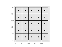
Figure 1: Cubic stratification in dimension $s=5$, with $k=5$, $N=25$. The black dots represent the centers $c_{n}$.

If $f\in\mathcal{C}^{1}\left([0,1]^{s}\right)$, then $\|f-\widehat{f}_{N}\|_{\infty}=\mathcal{O}(k^{-1})=\mathcal{O}(N^{1/s})$, and, by (2), the corresponding estimator is optimal for $r=1$. It turns out that one can obtain the same rate with a simpler estimator, as explained in the next section. Still, it will be useful in what comes next to keep this particular control variate in mind.

1.3 Stratification and optimal rates

Stratification is another well-known variance reduction strategy in Monte Carlo, see, e.g. Chap. 4 of Lemieux, (2009) or Chap. 8 of Owen, (2018). It amounts to splitting the integration domain into $P$ strata, and (assuming that the strata have the same volume, and that $P$ divides $N$), to generate in each stratum $N/P$ points.

Consider in particular as strata the $N$ sub-cubes mentioned in the previous section; that is, consider the following estimator:

$$\widehat{I}_{\mathrm{Haber}}=\frac{1}{N}\sum_{n=1}^{N}f(X_{n}),\qquad X_{n}\sim\mathcal{U}\left(C_{n}\right).$$

This estimator has been proposed by Haber, (1966) and is commonly referred to as the Haber estimator of order one. Note the similarity with the control variate estimator mentioned at the end of the previous section. It is easy to check that it has the same convergence rate, $\mathcal{O}(N^{-1/2-1/s})$, for $f\in\mathcal{C}^{r}\left([0,1]^{s}\right)$, and is therefore optimal as well (for $r=1$). In practice, Haber’s estimator is cheaper to compute (as it relies on $N$ evaluations, rather than $2N$), and has lower variance (as can be shown by a simple Rao-Blackwell argument). More generally, it is worth noting that control variates and stratification are very close in spirit, and especially so when the considered control variate is piecewise constant.

Haber’s estimator has been generalised to $r=2$ by Haber, (1967), and to $r\geq 3$ by Chopin and Gerber, (2024). The main drawback of these estimators is that they are defined only for $N=k^{s}$, $k=2,\ldots$. This is impractical whenever $s\gg 10$. Even when $s\leq 10$, dividing the domain into equal strata may be sub-optimal whenever $f$ vary more in certain directions than in others. Consider the extreme case where $s=2$, and $f$ is constant in the first component of $x$, but in the second. Then it would make more sense to slice the domain $[0,1]^{2}$ into $N$ horizontal slices, i.e., $[0,1]\times[(n-1)/N,n/N]$ for $n=1,\dots,N$.

1.4 Proposed approach

We develop in this paper an adaptive stratified Monte Carlo approach, where the strata are automatically adapted to the integrand $f$. To that effect, we generate a preliminary sample of size $N$ (as in control variates), and we train a decision (regression) tree on this data to construct the strata.

Decision trees are particularly convenient in our context, for two reasons, one fundamental, and one computational. The fundamental reason is that the regression function derived from a decision tree is piecewise constant, with ‘pieces’ constructed recursively in order to minimise the variance of the estimator. We use these ‘pieces’ as strata.

The practical one is that it learning and evaluating regression trees have complexity $\mathcal{O}(N\log N)$. Thus, the overall complexity of our approach will also be $\mathcal{O}(N\log N)$, which is more appealing than the polynomial complexity of approaches based on non-parametric control variates (again, see Oates et al.,, 2017; Leluc et al.,, 2023).

Finally, our approach will work for any sample size $N=2^{k}$, and could be extended easily to any arbitrary value of $N$, as we shall explain.

1.5 Plan and notations

Section˜2 presents decision trees, and describes the proposed estimator. Section˜3 develops some supporting theory for the proposed estimator. Section˜4 presents a numerical study to determine how practical and efficient is the proposed estimator. Section˜5 discusses future research. An appendix contains proofs of the main results.

We use the short-hand $1:N$ for the set of integers $\{n:\,1\leq n\leq N\}$. For $x\in\mathbb{R}^{s}$, we write its $j$-th component as $x[j]$. For any finite set $\mathcal{A}$ of points in $\mathbb{R}^{s}$, of size $|\mathcal{A}|$, we denote by $\operatorname{Average}(\mathcal{A})$ their average (empirical mean), assuming $|\mathcal{A}|\geq 1$, and by $\operatorname{EmpVar}(\mathcal{A})$ their empirical variance:

$$\operatorname{EmpVar}(\mathcal{A})=\frac{1}{|\mathcal{A}|-1}\sum_{x\in\mathcal{A}}\{x-\operatorname{Average}(\mathcal{A})\}^{2}$$

assuming $|\mathcal{A}|\geq 2$. In case $|\mathcal{A}|\leq 1$, we abuse notations and set $\operatorname{EmpVar}(\mathcal{A})=+\infty$. This non-standard convention will be convenient in the specific context of this paper.

We denote by $\operatorname{RMSE}\left(\widehat{I}_{\mathrm{}}\right)$ the RMSE of an estimator $\widehat{I}_{\mathrm{}}$. Since we deal only with unbiased estimator, this quantity is always the square root of $\mathrm{var}(\widehat{I})$, the variance of $\widehat{I}$.

2 Proposed algorithm

2.1 Decision trees

Decisions trees are classical supervised learning methods, which go back to Morgan and Sonquist, (1963). We focus on regression decision trees, which, given data $(X_{n},Y_{n})_{n=1,\dots,N}$, taking values in $[0,1]^{s}\times\mathbb{R}$, constructs a piecewise constant predictor:

$$\widehat{f}_{N}(x)=\sum_{p=1}^{P}y_{p}\times\mathds{1}\{x\in R_{p}\},\qquad y_{p}=\operatorname{Average}\{Y_{n}:\,X_{n}\in R_{p}\}$$ (3)

based on a partition of the feature space, $[0,1]^{s}$, which corresponds to a collection $\mathcal{R}=(R_{p})_{p=1,\dots,P}$ of rectangles (multi-variate intervals).

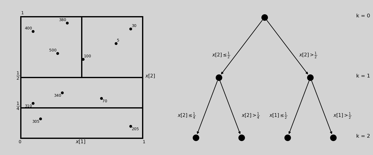
Figure 2: Partition of $[0,1]^{2}$ into rectangles (left) that correspond to a decision tree (right).

This collection is constructed by growing greedily (recursively) a tree, where each node corresponds to a simple rule, $X[j]\leq a$ or $X[j]>a$, and the leaves of the tree defines the rectangles $R_{p}$; see Fig.˜2. Given a rectangle $R$, let $R[j]^{+}$ and $R[j]^{-}$ define the two (equal size) sub-rectangles obtained by splitting $R$ in the middle, along axis $j$. That is, if $R=\prod_{i=1}^{s}[a_{i},b_{i}]$, then $R[j]^{-}=\prod_{i=1}^{s}[a_{i}^{\prime},b_{i}^{\prime}]$, with $(a_{i}^{\prime},b_{i}^{\prime})=\left(a_{i}^{\prime},b_{i}^{\prime}+(b_{i}^{\prime}-a_{i}^{\prime})/2\right)$ if $i=j$, $(a_{i}^{\prime},b_{i}^{\prime})=(a_{i},b_{i})$ otherwise; and $R[j]^{+}$ is defined similarly.

We initialise $\mathcal{R}$ as follows: $\mathcal{R}\leftarrow\{[0,1]^{s}\}$. Then, recursively, we replace each rectangle $R$ in $\mathcal{R}$ by $R[j_{\star}]^{+}$ and $R[j_{\star}]^{-}$, where $j_{\star}=\arg\min_{j\in 1:s}\widehat{\Delta}(R,j)$, and $\widehat{\Delta}(R,j)$ is the so-called CART (classification and regression tree) criterion:

$$\widehat{\Delta}(R,j):=\frac{1}{2}\operatorname{EmpVar}\{Y_{j}:X_{j}\in R[j]^{+}\}+\frac{1}{2}\operatorname{EmpVar}\{Y_{j}:X_{j}\in R[j]^{-}\}.$$ (4)

In words, we are trying to construct recursively a partition such that the $Y_{i}$ have as little variability as possible within each stratum.

We stop the splitting when the have reached a (pre-specified) depth $d$ (in that case, the volume of the considered rectangle is $2^{-d}$). In case of equality (more than one component $j$ achieves the smallest CART criterion), we choose randomly. This happens in particular when a given rectangle contains less than two points; then $\widehat{\Delta}(R,j)=\infty$ for all $j$, and again we choose randomly $j_{\star}$ among $1,\dots,s$.

We have described only one particular, simple way to learn a decision tree. Variants may be obtained by considering a criterion different from (4); by allowing to split at an arbitrary location (rather than in the middle); or by introducing pruning procedures (where the tree is grown until it reaches a certain depth, then some of its branches are pruned according to another criterion). For more details on all these variants, we refer to Chap. 9 of Hastie et al., (2009). The particular version we have focused on this section happens to fit well with our approach, as we explain in next section.

2.2 Proposed estimator

We now describe our approach. We assume $N=2^{k}$, for a certain integer $k\geq 1$. We proceed in two steps.

In the first step, we generate $N$ independent random variates $X_{n}\sim\mathcal{U}[0,1]^{s}$, we let $Y_{n}=f(X_{n})$, and we use the data $(X_{n},Y_{n})_{n\in[N]}$ to learn a decision tree, as explained in the previous section. We obtain a collection of rectangles $(R_{p})_{p\in 1:P}$. By construction, the volume of $R_{p}$ is $2^{-d}$ where $d$ is the depth of the tree, and $P=2^{d}$.

In a second step, we generate independently, for each $p$, and for $n=1,\dots,N_{p}:=N2^{-d}$, variate $\tilde{X}_{n,p}\sim\mathcal{U}(R_{p})$. The proposed estimator (called AdaStrat, for adaptive stratification) is then:

$$\widehat{I}_{\mathrm{AdaStrat}}=\frac{1}{N}\sum_{p=1}^{P}\sum_{n=1}^{N_{p}}f(\tilde{X}_{n,p})\qquad\tilde{X}_{n,p}\sim\mathcal{U}(R_{p}),$$ (5)

and it requires $2N$ evaluations of function $f$.

The whole procedure depends on a single tuning parameter, $d$, the maximum depth of the tree. In practice, we set $d=k$, which means that $P=N$. In a standard use of decision trees, this would presumably lead to over-fitting, in particular because rectangles obtained at a depth close to $k$ may contain too few points to estimate properly the optimal splitting directions. Note however that, in our context, splitting a retangle (i.e. replacing one stratum by two smaller strata) always reduce the variance of the stratified estimator. We will return to his point in our convergence study, in Section˜3.

2.3 Generalisation to any $N$

One limitation of our approach is that it requires $N$ to be a power of two, $N=2^{k}$. To generalise it to an arbitrary $N$, we can adapt the first step as follows. We initialise again our collection of rectangles as $\mathcal{R}=\left\{[0,1]^{s}\right\}$. Then we split recursively the rectangles in $\mathcal{R}$ in a way that ensures that the volume of each rectangle is always of the form $n_{R}/N$, where $n_{R}\in\mathbb{N}^{+}$.

Specifically, given a rectangle $R$ of volume $n_{R}/N$, let $R[n^{+},j]^{+}$ and $R[n^{-},j]^{+}$, be the two sub-rectangles obtained by splitting $R$ along axis $j$, at cut-point $n^{-}/n_{R}$; the volume of $R[n^{+},j]^{+}$ (resp. $R[n^{-},j]^{-}$) is then $n^{+}/N$ (resp. $n^{-}/N$), with $n^{+}+n^{-}=n_{R}$. In practice, we choose $(n^{+},j)$ so as to minimise:

$$\widehat{\Delta}(R,n^{+},j):=\frac{n^{+}}{n_{R}}\operatorname{EmpVar}\{Y_{j}:X_{j}\in R[n^{+},j]^{+}\}\\ +\frac{(n_{R}-n^{-})}{n_{R}}\operatorname{EmpVar}\{Y_{j}:X_{j}\in R[n_{R}-n^{+},j]^{-}\}.$$

This is very close to the standard variant of decision trees where one optimises with respect to both the direction, $j$, and the cut-point. However, in our case, we need to impose that the cut-point is $n^{+}/n_{R}$ for a certain $n^{+}\in\mathbb{N}^{+}$. In this way, when the tree is fully grown, we obtain a partition made of rectangles $R$, whose volume again is of the form $n_{R}/N$, and, in the second step, we may simply generate $n_{R}$ uniform variates in each rectangle $R$.

For the sake of simplicity, we focus on the $N=2^{k}$ version from now on.

3 Convergence study

Our objective in this section is to establish that the RMSE of (5) converges at a rate faster than $\mathcal{O}(N^{-1/2})$ for certain classes of functions. We proceed in two steps: first, we obtain convergence rates for a estimator based on an oracle tree; that is a tree which would be constructed as in Section˜2.1, but with empirical variances replaced by true variances. And, second, we study the impact of replacing the oracle tree by an ‘estimated’ one.

Before we start, we discuss very briefly the state of the art regarding the convergence of decision trees, and its relevance to our study.

3.1 Relation to the existing literature

Given the connection between stratification and control variates discussed in the introduction, see Section˜1.2, we thought initially of adapting existing results on the consistency (and rates of convergence) of decision trees to obtain RMSE rates for our stratified estimators. However, we found it easier in the end to establish ours results directly, from first principles. We think this is due to two factors.

First, establishing the consistency of approaches that rely on trees and greedy algorithms is challenging. We refer in particular to the the review of Biau and Scornet, (2016), who discusses the important gap between theory and practice for such methods (including random forests, which are a generalisation of decision trees), and to Scornet et al., (2015), who establishes the consistency of the corresponding estimates when the true function is additive. In other words, existing results apply to small classes of functions.

Second, our settings are actually simpler in several ways that the ones considered in the statistical literature: the true function $f$ is observed without noise in our case; we only allow binary splits in a given direction (rather than splits at an arbitrary cut-point); and, while pruning is essential in the standard use of decision trees (in order to avoid over-fitting), it is unnecessary in our case. This is because splitting a stratum into two strata always reduce the variance of our estimator. The pruning step is one of the factors that make the study of decision tree estimates challenging.

3.2 Oracle trees

We call oracle tree a tree obtained by the same procedure as in Section˜2.1, except that criterion $\widehat{\Delta}(R,j)$, see (4), is replaced by its theoretical counterpart:

$$\Delta(R,j):=\frac{1}{2}\Delta\left(R[j]^{+}\right)+\frac{1}{2}\Delta\left(R[j]^{-}\right),\quad\text{ with }\Delta(R):=\mathrm{var}\left[f(X)\middle|X\in R\right],$$

and the depth of the tree is set to $k$, so that the number of rectangles in the final partition is exactly $N=2^{k}$, and each rectangle has volume $1/N$. Let

$$\widehat{I}_{\mathrm{oracle}}=\frac{1}{N}\sum_{n=1}^{N}f(\widetilde{X}_{n}),\quad\widetilde{X}_{n}\sim\mathcal{U}(R_{n})$$

be the corresponding estimator.

Of course, this estimator is not implementable in practice, but its convergence rate gives us a lower bound on the error rate for the actual procedure. We start with a basic result.

Theorem 1.

Assume $f(x)=\lambda^{\top}x$, with $\lambda\in\mathbb{R}^{s}$ such that $\|\lambda\|_{0}=s_{0}\leq s$. Then

$$\operatorname{RMSE}\left(\widehat{I}_{\mathrm{oracle}}\right)=\mathcal{O}(N^{-1/2-r(s_{0})})$$

with $r(s_{0})=-\log(1-3/4s_{0})/2\log(2)\geq 0.541/s_{0}$.

This result strongly suggests that, while our approach may lead to higher convergence rates, it is not able to achieve the best possible rate, $1/2+1/r$ (assuming $s_{0}=s$) on the class of $\mathcal{C}^{1}\left([0,1]^{s}\right)$ functions.

On the other hand, the fact that the rate depends on $s_{0}$, the ‘actual’ dimension of $f$ indicates that our procedure is sparsity adaptive. This is hardly surprising, giving how the oracle tree is constructed: if $\lambda[j]=0$, then $\Delta(R,j)=0$ for any rectangle $R$, so one never splits along the $j$-th axis. Still, it is worth pointing out that, contrary to Haber’s estimator, or other methods based on a fixed stratification, our approach will automatically detect irrelevant dimensions.

We now turn our attention to a more general class of functions.

Theorem 2.

Assume $f$ is strictly increasing (with respect to each component), and that there exist real numbers $0<\alpha_{i}<\beta_{i}$, $i=1,\ldots,s$, such that, for all $x,y\in[0,1]^{s}$,

$$\Big{(}\sum_{i=1}^{s}\alpha_{i}^{2}(x_{i}-y_{i})^{2}\Big{)}^{1/2}\leq\left|f(x)-f(y)\right|\leq\Big{(}\sum_{i=1}^{s}\beta_{i}^{2}(x_{i}-y_{i})^{2}\Big{)}^{1/2}.$$

Then we have

$$\operatorname{RMSE}\left(\widehat{I}_{\mathrm{oracle}}\right)=\mathcal{O}(N^{-1/2-r(s)})$$

with

$$r(s)=\frac{1}{2\log 2}\log\left(\frac{\frac{3}{4}+\sum_{i=1}^{s}\frac{\beta^{2}_{i}}{\alpha^{2}_{i}}}{\sum_{i=1}^{s}\frac{\beta^{2}_{i}}{\alpha^{2}_{i}}}\right).$$

Note that for large $s$ and $\beta_{i}\to\alpha_{i}$, we obtain essentially the same rate as in ˜1.

The strongest assumption in ˜2 is the fact that $f$ must be strictly increasing in every direction. One may wonder whether this condition is really needed to obtain higher convergence rates. The following example shows that this is indeed the case.

Example 1.

Take $s=2$, and $f(x)=\lambda x[1]+\sin(2\pi x[2])$, for some $\lambda>0$. Then it is easy to see that the oracle tree will never split along the second direction, because doing so would keep the variance unchanged. As a result, the variance of $\widehat{I}_{\mathrm{oracle}}$ cannot converge faster than $\mathcal{O}(N^{-1/2})$.

We note in passing that is is easy to extend ˜2 to sparse functions, that is functions that are constant in certain components $i$; for such $i$, replace $\alpha_{i}$, $\beta_{i}$ and $\beta_{i}/\alpha_{i}$ by 0 in the expressions in that theorem. In that sense, that result is also "sparsity adaptive", as ˜1.

3.3 Estimated trees

To determine the behaviour of the actual estimator, we wish to study the probability that the estimated tree (constructed as explained in Section˜2.1) matches the oracle tree. This raises two issues however. First, if we split recursively the strata too many times, we end up with strata that contain a small number of points. The quantities $\widehat{\Delta}(R,j)$, used to decide along which axis one should split may become too noisy to ensure that the right direction is chosen. This suggests studying instead the probability that the oracle tree and the estimated tree matches only until a certain depth $L_{k}\ll k$.

Second, even we do so, we may have cases where the choice of the direction is a ‘close call’, that is, there exists $j\neq j^{\star}$ such that $\Delta(R,j)-\Delta(R,j^{\star})\ll 1$. (Consider for instance the first splitting operation when $f(x)=x[1]+0.99x[2]$.) In such a case, it is difficult to make the probability of taking the right decision large.

To deal with this technical issue, we define (for any $\varepsilon>0$) the notion of an $\varepsilon$-oracle tree, which is a tree constructed essentially as the oracle tree (using the theoretical criterion $\Delta(R,j)$ to decide which direction $j$ to pick), except in cases when, while splitting rectangle $R$, there exists a direction $j$ such that

$$\Delta(R,j)\leq\Delta(R,j^{\star})\frac{1+\varepsilon}{1-\varepsilon}.$$ (6)

In this situation, the $\varepsilon$-oracle is allowed to choose an arbitrary direction $j$ (among those $j$ such that (6) holds). We are able to show that the stratified estimator based on an $\varepsilon$-oracle converges at a slightly slower rate than the one based on the oracle tree.

With this approach, we are able to obtain convergence rates for our actual estimator under essentially the same conditions as for the oracle estimator.

Theorem 3.

Consider the set-up of ˜2. Then, one has

$$\operatorname{RMSE}\left(\widehat{I}_{\mathrm{AdapStrat}}\right)=\mathcal{O}(N^{-1/2-r^{\prime}})$$

for any $0<r^{\prime}<r(s)$, where $r(s)$ is defined as in ˜2.

4 Numerical experiments

In this section, we compare our adaptive stratification estimator with the standard Monte Carlo estimator, $\widehat{I}_{\mathrm{MC}}$, and Haber estimator or order one, $\widehat{I}_{\mathrm{Haber}}$ when possible (recall that the last estimator is defined only for $N=k^{s}$, $k\geq 2$). Our comparison is in terms of relative RMSE (RMSE divided by true value, or an estimate based on a grand mean), and how it varies as a function of $N$. The RMSE is evaluated over 256 independent realisations of the estimators.

4.1 Toy example

We consider the following linear function $f(x)=\exp\{\sum_{i=1}^{s}\lambda_{i}x_{i}\}$, with decreasing weights, $\lambda_{i}=i^{-2}$. This way, component $i$ contributes less and less to the overall variance as $i$ grows; this is a favourable case for our adaptive stratification strategy.

Fig.˜3 compares the performance (i.e. RMSE vs $N$) of the following unbiased estimators when $s=5$: standard Monte Carlo, $\widehat{I}_{\mathrm{MC}}$, Haber of order one (defined in Section˜1), and our stratified estimator based on a decision tree grown either until depth $d=k$. Interestingly, our approach outperforms even Haber’s estimator, although the latter is supposed to converge at a higher rate. The dashed lines represents the theoretical convergence rates of the considered estimators.

Fig.˜4 does the same comparison for $s=15$ and $s=50$, but this time Haber’s estimate is omitted, as it is only defined for $N=k^{s}$, $k\geq 2$, and thus it cannot be computed for reasonable values of $N$ whenever $s\gg 10$. We note that our approach leads to a measurable improvement even when $s=50$.

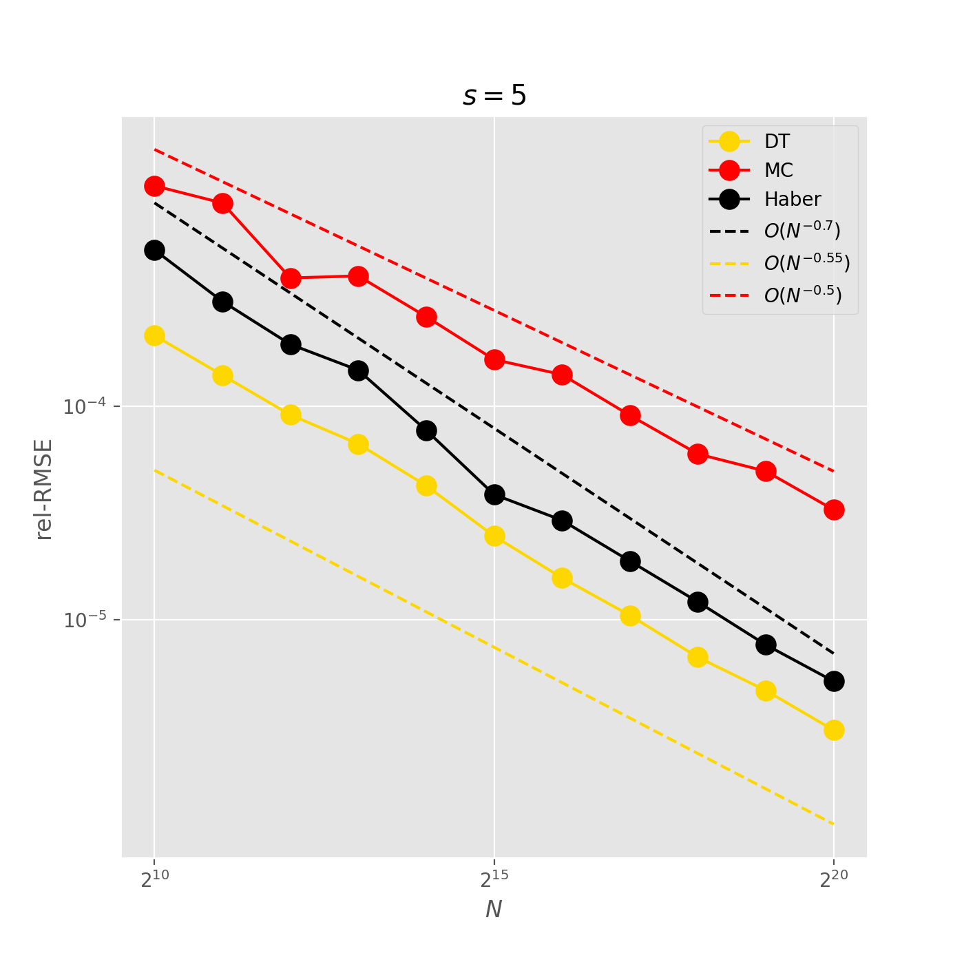
Figure 3: Toy example, $s=5$. RMSE vs $N$ (estimated from 256 independent realisations) for the following unbiased estimators: standard Monte Carlo (MC, red), Haber of order one (Haber, black), and our adaptive decision-tree strategy (DT, yellow). Dashed lines represent the theoretical convergence rates of these three estimators.

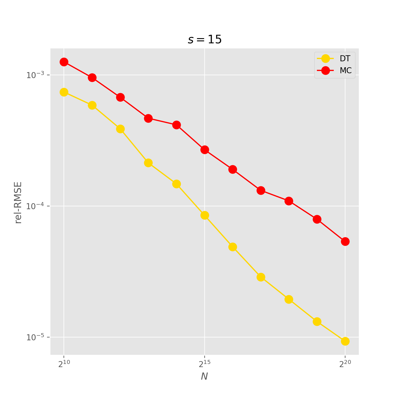
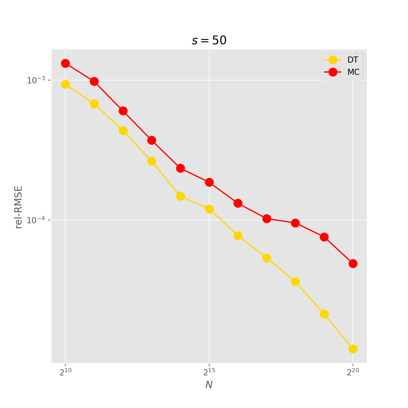
Figure 4: Toy example, $s=15$ (left) and $s=50$ (right). Same plot as Fig.˜3 except Haber estimator of order one has been excluded, and the theoretical convergence rates are not plotted for the sake of readability.

One advantage of stratification that we have not discussed in the body of the paper is that it is easy to estimate the variance of a stratified estimator, by generating two (instead of one) point in each stratum. The variance estimate is the sum (over the strata) of the empirical variance within each stratum. This idea was discussed in relation to Haber and related estimators in Chopin and Gerber, (2024). Figure˜5 compares box-plots of such variance estimates when $N=2^{10}$ and $s=5$ with the variance estimate of standard Monte Carlo. One can see that one obtains variance estimates that are far more stable.

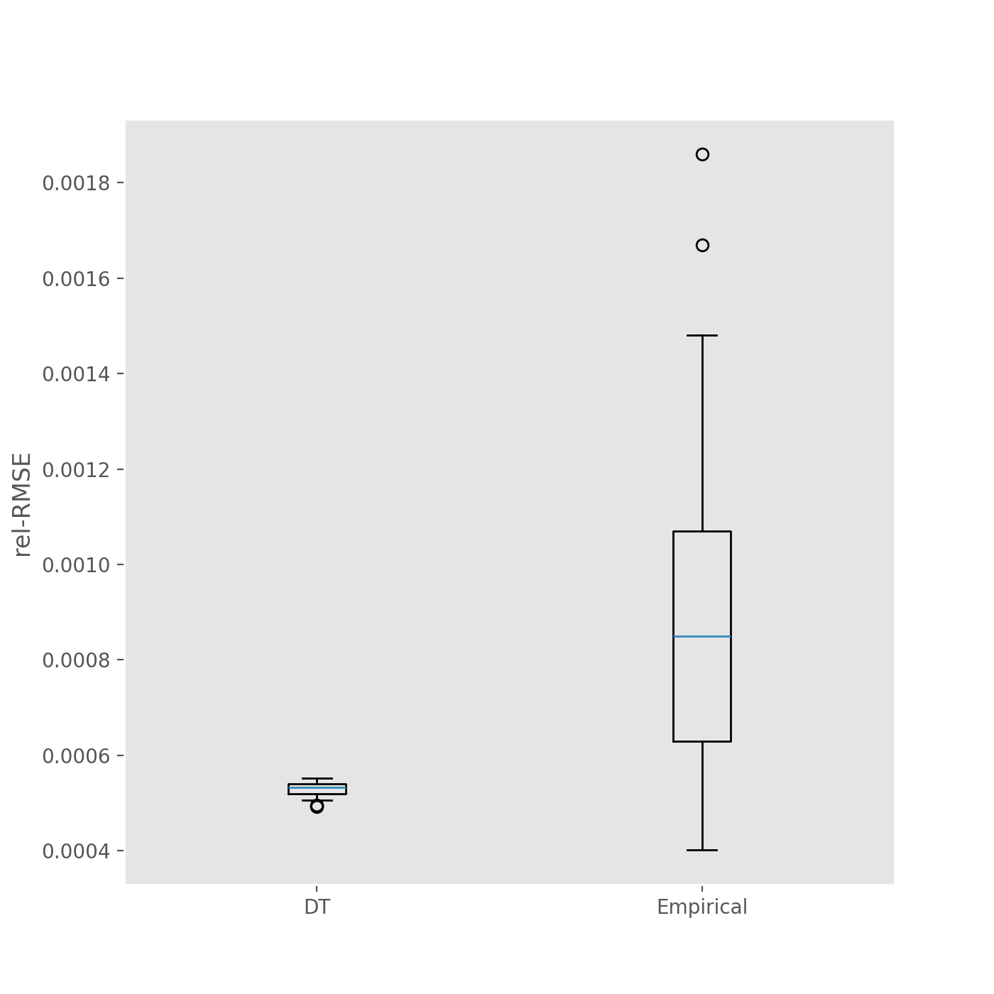
Figure 5: Toy example, $s=5$, $N=2^{10}$. Box-plots of variance estimates for the Monte Carlo estimator and our adaptive stratified estimator.

4.2 Bayesian model choice

We consider a Bayesian statistical model, with parameter $\beta\in\mathbb{R}^{d}$, prior distribution $p(\beta)$, and likelihood $L(y|\beta)$. We wish to approximate unbiasedly the marginal likelihood $p(y)=\int p(\beta)L(y|\beta)\,d\beta$. This quantity may be used to perform model choice. We adapt the importance sampling approach described in Chopin and Ridgway, (2017) to approximate marginal likelihoods as follows: we obtain numerically the mode $\hat{\beta}$, and the Hessian at $\beta=\hat{\beta}$, of the function $h(\beta)=\log\{p(\beta)L(y|\beta)\}$; hence $h(\beta)\approx h(\hat{\beta})-(1/2)(\beta-\hat{\beta})^{T}H(\beta-\hat{\beta})$. Then we set the importance density to $q(\beta)=N(h(\hat{\beta}),H^{-1})$. Finally, we rewrite the integral

$$p(y)=\mathbb{E}_{q}\left[\frac{p(\beta)L(y|\beta)}{q(\beta)}\right]=\int_{[0,1]^{s}}f(x)\mathop{}\!\mathrm{d}{x}$$

where $f(x)=\hat{\beta}+C\Phi^{-1}(x)$, $CC^{\top}=H^{-1}$ is the Cholesky decomposition of $H^{-1}$, and $\Phi^{-1}(x)$ is the vector of $\Phi^{-1}(x_{i})$’s, with $\Phi^{-1}$ being the the quantile (inverse CDF) function associated to the $N(0,1)$ distribution.

Specifically, we assume a Gaussian prior (with zero mean and covariance $5^{2}I_{s}$), and a logistic regression model: $L(y|\beta)=\prod_{i=1}^{n}F(y_{i}\beta^{T}x_{i})$, $F(z)=1/(1+e^{-z})$, and the data $(x_{i},y_{i})_{i=1}^{n}$ consist of predictors $x_{i}\in\mathbb{R}^{s}$ and labels $y_{i}\in\{-1,1\}$. We use the German credit dataset from the UCI machine learning repository, and the $s$ first predictors, for $s=5$, $10$, $15$, $20$. Predictors are rescaled to have mean zero and variance one.

Figure 6 compares our estimators with the standard MC (Monte Carlo) estimator for $s=5$, 10, 15 and 20. Whatever the dimension, we see a distinctive improvement with our method.

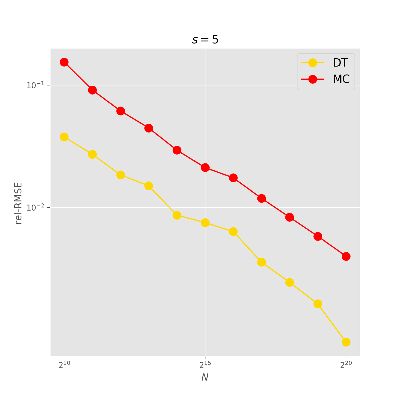
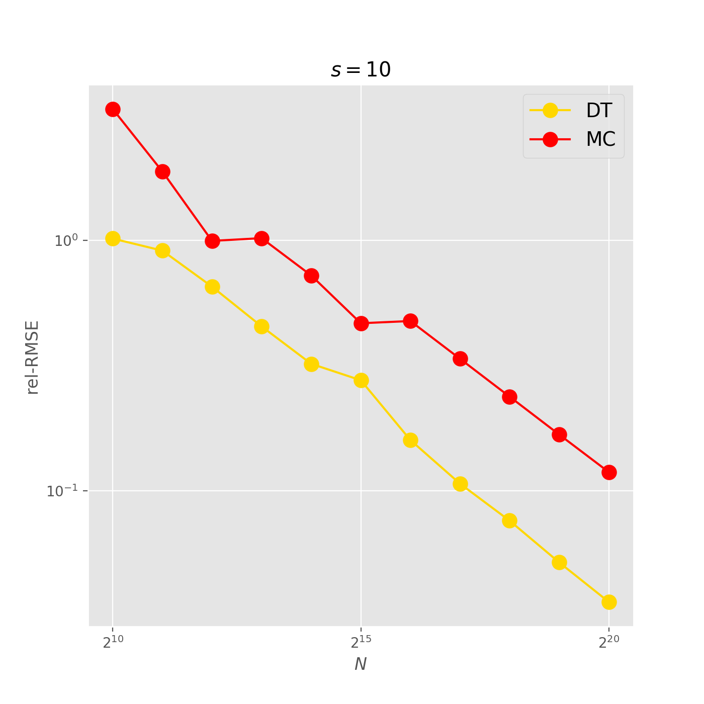
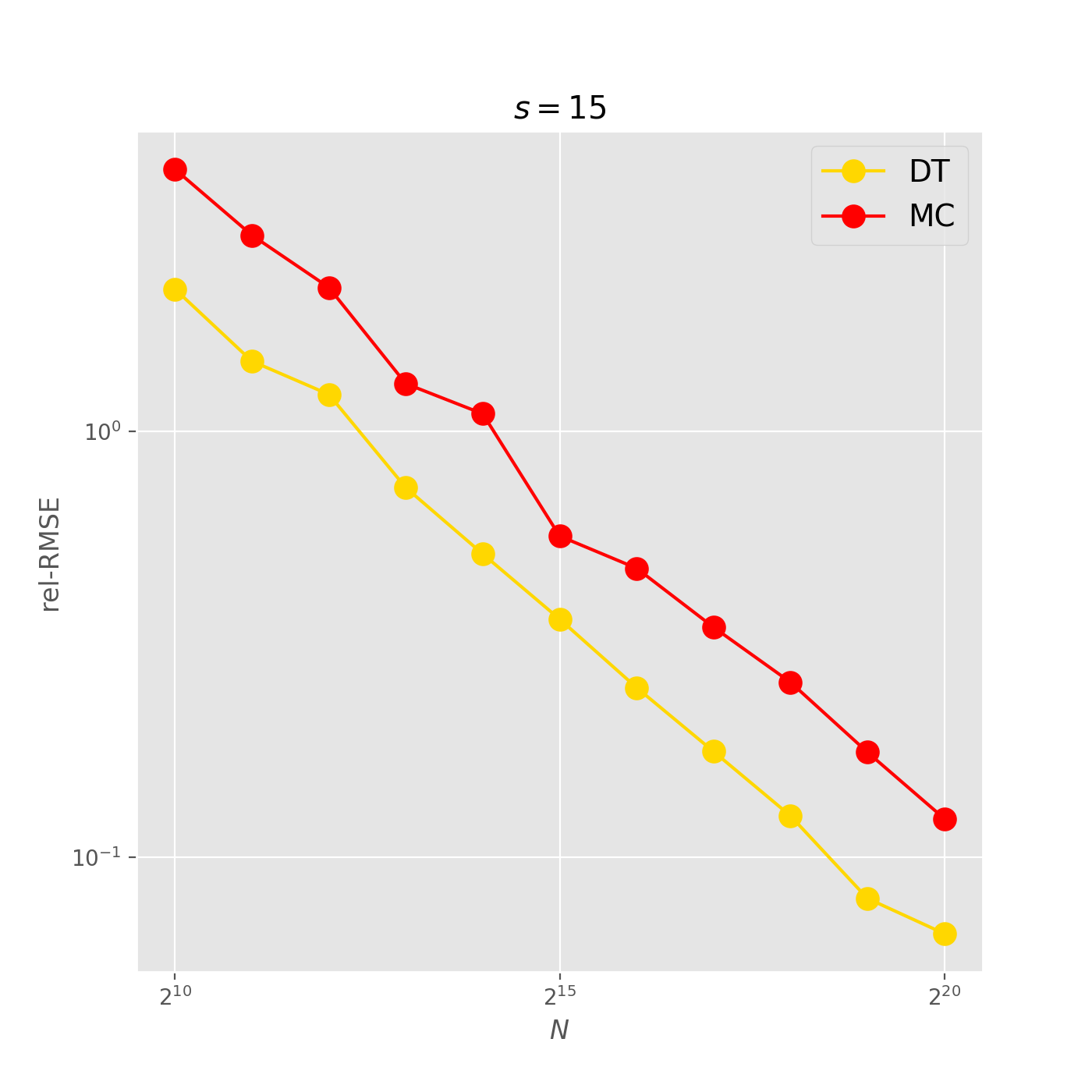
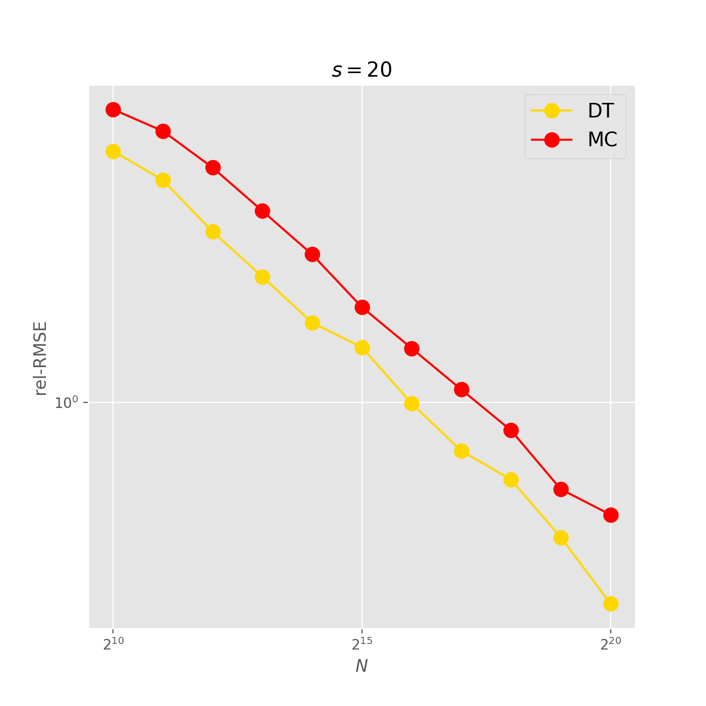
Figure 6: Bayesian model choice example, $s=5$, $10$, $15$, $20$: RMSE (over 256 independent realisations) versus $N$ for the following unbiased estimators: standard Monte Carlo (MC, red), and our adaptive stratified Monte Carlo estimators (DT, yellow).

5 Discussion and future work

The strategy developed in this paper represents an important step towards making stratified Monte Carlo more practical, especially in moderate to high dimensions. Its main limitation is that it does not reach the optimal convergence rate for $\mathcal{C}^{r}$ functions, even for $r=1$. It remains to be seen whether one can obtain such rates with a tree-based approach. More generally, we suspect that the decision trees and their generalisations such as random forest may find other uses in Monte Carlo computation (e.g., control variates), in particular because of the low complexity of their learning procedures.

Proofs

Proof of ˜1

We consider a sequence of stratified estimators, $\widehat{I}_{0},\widehat{I}_{1},\dots$, which corresponds to a sequence of sets of rectangles $\mathcal{R}_{0},\mathcal{R}_{1},\dots$, starting at $\mathcal{R}_{0}=\{[0,1]^{s}\}$ (hence $\widehat{I}_{0}=\widehat{I}_{\mathrm{MC}}$) and corresponding to the successive splitting operations performed while growing the tree, as described in Section˜2.1: that is, at each iteration, takes a rectangle $R$ in $\mathcal{R}_{t}$ and replace it by two rectangles, $R[j^{\star}]^{+}$ and $R[j^{\star}]^{-}$, where $j^{\star}$ is the index that leads to greatest variance reduction.

These stratified estimators $\widehat{I}_{0}$, $\widehat{I}_{1}$, $\dots$ are defined as

$$\widehat{I}_{t}=\frac{1}{N}\sum_{R\in\mathcal{R}_{t}}\sum_{n=1}^{n_{R}}f(X_{p,n}),\qquad X_{p,n}\sim\mathcal{U}(R_{p}),$$

where $n_{R}=N\times\operatorname{Vol}(R)$, hence their variance has the form:

$$\frac{1}{N}\sum_{R\in\mathcal{R}_{t}}\operatorname{Vol}(R)\times\Delta(R)$$

where $\Delta(R)=\mathrm{var}\left[f(X)\middle|X\in R\right]$, where the conditional distribution is taken with respect to $X\sim\mathcal{U}([0,1])$. Thus, splitting a particular rectangle amounts to replacing one term in this expression by a sum of two terms, leading to the variance reduction factor:

$$\frac{\Delta(R[j^{\star}]^{+})+\Delta(R[j^{\star}]^{-})}{2\Delta(R)}.$$ (7)

Elementary calculations show that, if $f(x)=\lambda^{T}x$, and rectangle $R$ has dimensions $\mu_{1}\times\dots\times\mu_{s}$, then $\Delta(R)=\sum_{j=1}^{s}\mu_{j}^{2}\lambda_{j}^{2}/12$. In that case, ratio (7) equals:

$$\frac{\Delta(R[j^{\star}]^{+})+\Delta(R[j^{\star}]^{-})}{2\Delta(R)}=1-\frac{3\mu_{j^{\star}}^{2}\lambda_{j^{\star}}^{2}}{4\sum_{j=1}^{s}\mu_{j}^{2}\lambda_{j}^{2}}\leq 1-\frac{3}{4s_{0}}.$$

The inequality comes from $j^{\star}=\arg\min_{j=1,\dots,s}\{\Delta(R[j]^{+})+\Delta(R[j]^{-})\}$, and the fact that the maximum of $s$ number is larger than their average.

At the end of the splitting process, where one has obtained $N$ rectangles of volume $1/N$ (recall that $d=k$ hence $P=2^{d}=2^{k}=N$), we get

$$\mathrm{var}[\widehat{I}_{\mathrm{oracle}}]\leq\left(1-\frac{3}{4s_{0}}\right)^{k}\mathrm{var}[\widehat{I}_{0}]$$

with $\mathrm{var}[\widehat{I}_{0}]=\mathcal{O}(N^{-1})$, and, since $N=2^{k}$,

$$\left(1-\frac{3}{4s_{0}}\right)^{k}=\exp\left\{\log(N)\times\frac{\log(1-3/4s_{0})}{\log 2}\right\}=N^{-2\alpha(s_{0})}$$

with $\alpha(s_{0})=-\log(1-3/4s_{0})/(2\log 2)\geq 3/(8s_{0}\log 2)$, since $\log(1+x)\leq x$.

Proof of ˜2

We follow the same lines as in the previous proof: given a rectangle $R$, we wish to bound variance reduction factor (7). We use the law of total variance formula to get (for any $j\in 1:s$):

$$\Delta(R)=\mathrm{var}\left[f(X)\middle|X\in R\right]=C_{1}+C_{2}$$ (8)

with

$$C_{1} :=\frac{1}{4}\Big{\{}\mathbb{E}\left[f(X)\middle|X\in R[j]^{+}\right]-\mathbb{E}\left[f(X)\middle|X\in R[j]^{-}\right]\Big{\}}^{2},$$

$$C_{2} :=\frac{1}{2}\mathrm{var}\left[f(X)\middle|X\in R[j]^{+}\right]+\frac{1}{2}\mathrm{var}\left[f(X)\middle|X\in R[j]^{-}\right].$$

To bound the first term, we remark that (assuming the dimensions of $R$ are $\mu_{1}\times\dots\times\mu_{s}$):

$$\mathbb{E}\left[f(X)\middle|X\in R[j]^{+}\right]-\mathbb{E}\left[f(X)\middle|X\in R[j]^{-}\right]\\ =\mathbb{E}\left[\left\{f(X+\frac{\mu_{j}}{2}e_{j})-f(X)\right\}\middle|X\in R[j]^{-}\right]\geq\frac{\alpha_{i}\mu_{j}}{2}$$

hence $C_{1}\geq\alpha_{j}^{2}\mu_{j}^{2}/16$.

To bound the second term, we remark that:

$$\mathrm{var}\left[f(X)\middle|X\in R\right] =\frac{1}{2}\mathbb{E}\left[\left\{f(X^{\prime})-f(X)\right\}^{2}\middle|X,X^{\prime}\in R\right]\leq\frac{1}{12}\sum_{i=1}^{s}\beta_{i}^{2}\mu_{i}^{2}.$$

If we apply this inequality to $R[j]^{+}$ and $R[j]^{-}$, we obtain:

$$C_{2} \leq\frac{1}{12}\sum_{i=1}^{s}\beta^{2}_{i}\mu_{i}^{2}=\frac{\alpha^{2}_{j}\mu^{2}_{j}}{12}\sum_{i=1}^{s}\frac{\beta^{2}_{i}}{\alpha^{2}_{i}}\,\frac{\alpha_{i}^{2}\mu_{i}^{2}}{\alpha^{2}_{j}\mu^{2}_{j}}.$$

Then, we can bound (7) as follows:

$$\frac{\Delta(R[j]^{+})+\Delta(R[j]^{-})}{2\Delta(R)}=\frac{C_{2}}{C_{1}+C_{2}} \leq\frac{\frac{\alpha^{2}_{j}\mu^{2}_{j}}{12}\sum_{i=1}^{s}\frac{\beta^{2}_{i}}{\alpha^{2}_{i}}\,\frac{\alpha_{i}^{2}\mu_{i}^{2}}{\alpha^{2}_{j}\mu^{2}_{j}}}{\frac{\alpha_{j}^{2}\mu_{j}^{2}}{16}+\frac{\alpha^{2}_{j}\mu^{2}_{j}}{12}\sum_{i=1}^{s}\frac{\beta^{2}_{i}}{\alpha^{2}_{i}}\,\frac{\alpha_{i}^{2}\mu_{i}^{2}}{\alpha^{2}_{j}\mu^{2}_{j}}}=\frac{\frac{4}{3}\sum_{i=1}^{s}\frac{\beta^{2}_{i}}{\alpha^{2}_{i}}\,\frac{\alpha_{i}^{2}\mu_{i}^{2}}{\alpha^{2}_{j}\mu^{2}_{j}}}{1+\frac{4}{3}\sum_{i=1}^{s}\frac{\beta^{2}_{i}}{\alpha^{2}_{i}}\,\frac{\alpha_{i}^{2}\mu_{i}^{2}}{\alpha^{2}_{j}\mu^{2}_{j}}}.$$

This inequality holds for all $j=1,\dots,s$, and in particular it holds for $j^{\star}=\arg\min\{\Delta(R[j]^{+})+\Delta(R[j]^{-})$. Therefore, noting that if we let $k=\mathrm{argmax}_{j\in\{1,\dots,s\}}\alpha_{j}^{2}\mu_{j}^{2}$ we have

$$\frac{\frac{4}{3}\sum_{i=1}^{s}\frac{\beta^{2}_{i}}{\alpha^{2}_{i}}\,\frac{\alpha_{i}^{2}\mu_{i}^{2}}{\alpha^{2}_{j}\mu^{2}_{j}}}{1+\frac{4}{3}\sum_{i=1}^{s}\frac{\beta^{2}_{i}}{\alpha^{2}_{i}}\,\frac{\alpha_{i}^{2}\mu_{i}^{2}}{\alpha^{2}_{j}\mu^{2}_{j}}}\geq\frac{\frac{4}{3}\sum_{i=1}^{s}\frac{\beta^{2}_{i}}{\alpha^{2}_{i}}\,\frac{\alpha_{i}^{2}\mu_{i}^{2}}{\alpha^{2}_{k}\mu^{2}_{k}}}{1+\frac{4}{3}\sum_{i=1}^{s}\frac{\beta^{2}_{i}}{\alpha^{2}_{i}}\,\frac{\alpha_{i}^{2}\mu_{i}^{2}}{\alpha^{2}_{k}\mu^{2}_{k}}},\quad\forall j\in\{1,\dots,s\}$$

it follows that

$$\frac{\Delta(R[j^{\star}]^{+})+\Delta(R[j^{\star}]^{-})}{2\Delta(R)} \leq\frac{\frac{4}{3}\sum_{i=1}^{s}\frac{\beta^{2}_{i}}{\alpha^{2}_{i}}\,\frac{\alpha_{i}^{2}\mu_{i}^{2}}{\alpha^{2}_{k}\mu^{2}_{k}}}{1+\frac{4}{3}\sum_{i=1}^{s}\frac{\beta^{2}_{i}}{\alpha^{2}_{i}}\,\frac{\alpha_{i}^{2}\mu_{i}^{2}}{\alpha^{2}_{k}\mu^{2}_{k}}}\leq\frac{\frac{4}{3}\sum_{i=1}^{s}\frac{\beta^{2}_{i}}{\alpha^{2}_{i}}}{1+\frac{4}{3}\sum_{i=1}^{s}\frac{\beta^{2}_{i}}{\alpha^{2}_{i}}}$$

where the second inequality uses the fact that $(\alpha_{i}^{2}\mu_{i}^{2})/(\alpha_{k}^{2}\beta_{k}^{2})\leq 1$ for all $i\in\{1,\dots,s\}$ and the fact that the function $x\mapsto x/(1+x)$ is non-decreasing on $[0,\infty)$.

We can now conclude in the same way as in the previous proof:

$$\mathrm{var}\left[\widehat{I}_{\mathrm{oracle}}\right] \leq\left(\frac{\sum_{i=1}^{s}\frac{\beta^{2}_{i}}{\alpha^{2}_{i}}}{\frac{3}{4}+\sum_{i=1}^{s}\frac{\beta^{2}_{i}}{\alpha^{2}_{i}}}\right)^{k}\mathrm{var}\left[\widehat{I}_{\mathrm{MC}}\right]$$ (9)

$$=\mathcal{O}(N^{-1-2r(s)})$$

with

$$r(s)=\frac{1}{2\log 2}\log\left(\frac{\frac{3}{4}+\sum_{i=1}^{s}\frac{\beta^{2}_{i}}{\alpha^{2}_{i}}}{\sum_{i=1}^{s}\frac{\beta^{2}_{i}}{\alpha^{2}_{i}}}\right).$$

Proof of ˜3

We consider some fixed $\varepsilon\in(0,1)$ throughout.

We first recall a concentration inequality due to Maurer and Pontil, (2009).

Proposition 1 (Theorem 10 in Maurer and Pontil,, 2009).

Let $Z_{1},\ldots,Z_{N}$ be IID random variables taking values in $[0,1]$, $\Delta=\mathrm{var}(Z)$, and

$$\widehat{\Delta}=\frac{1}{N-1}\sum_{n=1}^{N}(Z_{n}-\bar{Z})^{2},$$

the empirical variance. Then:

$$\mathbb{P}\left(\widehat{\Delta}^{1/2}>\Delta^{1/2}+\varepsilon\right) \leq\exp\left\{-\frac{(N-1)\varepsilon^{2}}{2}\right\},$$ (10)

$$\mathbb{P}\left(\widehat{\Delta}^{1/2}<\Delta^{1/2}-\varepsilon\right) \leq\exp\left\{-\frac{(N-1)\varepsilon^{2}}{2}\right\}.$$

A simple corollary of the above result is:

Lemma 1.

Let $Z_{1},\dots,Z_{N}$ IID variables taking values in some compact interval $[a,b]$, $\Delta$, $\widehat{\Delta}$ be defined as above, and $\gamma:=(1+\varepsilon)^{1/2}-1$. Then (assuming $\Delta>0$):

$$\mathbb{P}\left(\frac{\widehat{\Delta}}{\Delta}>1+\varepsilon\right) \leq\exp\left\{-\frac{(N-1)\Delta\gamma^{2}}{2(b-a)^{2}}\right\},$$

$$\mathbb{P}\left(\frac{\widehat{\Delta}}{\Delta}<1-\varepsilon\right) \leq\exp\left\{-\frac{(N-1)\Delta\gamma^{2}}{2(b-a)^{2}}\right\}.$$

Proof.

Inequality $\widehat{\Delta}>\Delta(1+\varepsilon)$ is equivalent to

$$\widehat{\Delta}^{1/2}>\Delta^{1/2}+\Delta^{1/2}\{(1+\varepsilon)^{1/2}-1\}$$

the probability of which may be bounded by applying Eq.˜10 to the rescaled variables $Z_{n}^{\prime}=(Z_{n}-a)/(b-a)$, and replacing $\varepsilon$ with $\Delta^{1/2}\gamma$, with $\gamma=(1+\varepsilon)^{1/2}-1$. ∎

We can now apply this lemma to the set of $f(X_{n})$ for those $X_{n}$ that fall in a given rectangle $R$.

Lemma 2.

Let $R$ a rectangle included in $[0,1]^{s}$, of volume $2^{-l}$. Then, under the same conditions as in ˜2,

$$\mathbb{P}\left(\frac{\widehat{\Delta}(R)}{\Delta(R)}\geq 1+\varepsilon\right)\leq e^{\kappa}\left[1-2^{-l}(1-e^{-\kappa})\right]^{N}$$

where $\kappa:=\gamma^{2}\alpha^{2}/12\beta^{2}$, $\gamma=(1+\varepsilon)^{1/2}-1$, $\alpha=\inf_{i\in\{1,\dots,s\}}\alpha_{i}$ and $\beta\max_{i\in\{1,\dots,s\}}\beta_{u}$. This inequality also holds for $\mathbb{P}\left(\frac{\widehat{\Delta}(R)}{\Delta(R)}\leq 1-\varepsilon\right)$.

Proof.

Let $N(R)=\sum_{n=1}^{N}\mathds{1}\{X_{n}\in R\}$. Conditional on $N(R)=n$, the $n$ variates $X_{n}$ that fall in $R$ follow an uniform distribution with respect to $R$. Therefore, from ˜1, one has:

$$\mathbb{P}\left(\frac{\widehat{\Delta}(R)}{\Delta(R)}\geq 1+\varepsilon\middle|N(R)=n\right) \leq\exp\left\{-\frac{(n-1)\Delta(R)\gamma^{2}}{2D(R)}\right\}$$

$$\leq\exp\left\{-(n-1)\frac{\gamma^{2}\alpha^{2}}{12\beta^{2}}\right\}$$

$$\leq e^{\kappa}\exp\left\{-n\kappa\right\}$$

where in the first line, $D(R)=\left(\sup_{x,y\in R}|f(y)-f(x)|\right)^{2}$, and, in the second line, we have used

$$\Delta(R)\geq\frac{\alpha^{2}}{2}\mathbb{E}\left[\|X-Y\|^{2}\middle|X,Y\in R\right]=\frac{\alpha^{2}}{12}\sum_{i=1}^{s}\mu_{i}^{2}$$ (11)

and $D(R)\leq\beta^{2}\sum_{i=1}^{s}\mu_{i}^{2}$, assuming that $R$ has dimensions $\mu_{1}\times\dots\times\mu_{s}$. Since $N(R)\sim\mathrm{Bin}(N,2^{-l})$, one has, for any $c>0$: $\mathbb{E}[\exp\{-cN(R)\}]=[1-2^{-l}+2^{-l}\exp(-c)]^{N}$, which gives the desired result. The second inequality may be established in the same way. ∎

We can now proceed with the proof of the theorem. The gist of the proof is to show that the probability that the estimated tree is an $\varepsilon$-oracle is close to one. Consider a rectangle $R$, of volume $2^{-l}$ (i.e., it has been obtained through $l$ splitting operations), and assume that (6) does not hold for any $j$. Then, one chooses the right coordinate, $j^{\star}=\arg\min_{j=1,\dots,s}\Delta(R,j)$ as soon as: for all $j\neq j^{\star}$, $\widehat{\Delta}(R[j]^{+})\geq\Delta(R[j]^{+})(1-\varepsilon)$, the same is true for $R[j]^{-}$, and, in addition, $\widehat{\Delta}(R[j^{\star}]^{+})\leq\Delta(R[j^{\star}]^{+})(1+\varepsilon)$, and the same holds for $R[j^{\star}]^{-}$.

Conversely, using the union bound and ˜2, we see that the probability of not choosing the right coordinate (when splitting $R$) is bounded by

$$2se^{\kappa}\left(1-2^{-l-1}e^{-\kappa}\right)^{N}$$

with the constant $\kappa>0$ as defined in ˜2.

More generally, the probability $p_{k,L}$ of making at least one ‘wrong’ decision while constructing the tree (i.e. constructing a tree that is an $\varepsilon$-oracle), until depth $L$, is such that

$$\begin{split}p_{k,L}\leq 2se^{\kappa}\sum_{l=1}^{L}2^{l}\left(1-2^{-l}e^{-\kappa}\right)^{N}&\leq 2se^{\kappa}L2^{L}\left(1-2^{-L}e^{-\kappa}\right)^{N}\\ &\leq 2se^{\kappa}\exp\left\{\log L+L\log 2-2^{k-L}e^{-\kappa}\right\}.\end{split}$$ (12)

Remark that for all $\delta\in(0,\infty)$ we have

$$\exp\big{(}-\delta 2^{k-L}\big{)}\leq 2^{-2k}\Leftrightarrow L\leq k-\frac{\log(2k/\delta)}{\log(2)}-\frac{\log(\log(2))}{\log(2)}.$$

Take $L_{k}=\lfloor k-c\log(k)^{1+\gamma}\rfloor$ for some constants $c\in(0,\infty)$ and $\gamma\in(0,1)$. Then

$$\exp\big{(}-2^{k-L_{k}}e^{-\kappa}\big{)}\leq 2^{-2k}=N^{-2}.$$ (13)

In words, the probability that the estimated tree and the $\varepsilon-$oracle tree differ before depth $L_{k}$ is $\mathcal{O}(N^{-2})$. Beyond depth $L_{k}$, we let the $\varepsilon-$oracle tree choose arbitrarily the split decisions; this leads to variance reduction factors which equal 1 in the worst case (splitting always reduce the variance).

We conclude the proof by remarking that replacing the oracle by an $\varepsilon$-oracle degrades the convergence rate by a certain amount. More precisely, adapting (9) leads to

$$\mathrm{var}\left[\widehat{I}_{\varepsilon-\mathrm{oracle}}\right] \leq\left(\frac{\sum_{i=1}^{s}\frac{\beta^{2}_{i}}{\alpha^{2}_{i}}}{\frac{3}{4}+\sum_{i=1}^{s}\frac{\beta^{2}_{i}}{\alpha^{2}_{i}}}\times\frac{1+\varepsilon}{1-\varepsilon}\right)^{L_{k}}$$

$$=\left\{\left(\frac{\sum_{i=1}^{s}\frac{\beta^{2}_{i}}{\alpha^{2}_{i}}}{\frac{3}{4}+\sum_{i=1}^{s}\frac{\beta^{2}_{i}}{\alpha^{2}_{i}}}\times\frac{1+\varepsilon}{1-\varepsilon}\right)^{1-(1-L_{k}/k)}\right\}^{k}$$

$$\leq\left\{\left(\frac{\sum_{i=1}^{s}\frac{\beta^{2}_{i}}{\alpha^{2}_{i}}}{\frac{3}{4}+\sum_{i=1}^{s}\frac{\beta^{2}_{i}}{\alpha^{2}_{i}}}\times\frac{1+\varepsilon}{1-\varepsilon}\right)^{1-\varepsilon}\right\}^{k}$$

where the last inequality holds for $k$ large enough. This shows that $\mathrm{var}[\widehat{I}_{\mathrm{MC}}]=\mathcal{O}(N^{-1-2r^{\prime}_{\varepsilon}})$ with

$$r_{\varepsilon}^{\prime}=-\frac{1-\varepsilon}{2\log 2}\log\left(\frac{\sum_{i=1}^{s}\frac{\beta^{2}_{i}}{\alpha^{2}_{i}}}{\frac{3}{4}+\sum_{i=1}^{s}\frac{\beta^{2}_{i}}{\alpha^{2}_{i}}}\times\frac{1+\varepsilon}{1-\varepsilon}\right)<r(s).$$

Since $\varepsilon\in(0,1)$ is arbitrary one can make $r_{\varepsilon}^{\prime}$ as close as $r(s)$ as desired.

References

- Andrieu and Roberts, (2009) Andrieu, C. and Roberts, G. O. (2009). The pseudo-marginal approach for efficient Monte Carlo computations. Ann. Statist., 37(2):697–725.
- Bahvalov, (1959) Bahvalov, N. S. (1959). Approximate computation of multiple integrals. Vestnik Moskov. Univ. Ser. Mat. Meh. Astr. Fiz. Him., 1959(4):3–18.
- Biau and Scornet, (2016) Biau, G. and Scornet, E. (2016). A random forest guided tour. TEST, 25(2):197–227.
- Chopin and Gerber, (2024) Chopin, N. and Gerber, M. (2024). Higher-order Monte Carlo through cubic stratification. SIAM J. Numer. Anal., 62(1):229–247.
- Chopin and Ridgway, (2017) Chopin, N. and Ridgway, J. (2017). Leave Pima Indians alone: binary regression as a benchmark for Bayesian computation. Statist. Sci., 32(1):64–87.
- Haber, (1966) Haber, S. (1966). A modified Monte-Carlo quadrature. Mathematics of Computation, 20(95):361–368.
- Haber, (1967) Haber, S. (1967). A modified Monte-Carlo quadrature. ii. Mathematics of Computation, 21(99):388–397.
- Hastie et al., (2009) Hastie, T., Tibshirani, R., and Friedman, J. (2009). The elements of statistical learning, volume 2 of Springer Series in Statistics. Springer, New York, second edition. Data mining, inference, and prediction.
- Leluc et al., (2023) Leluc, R., Portier, F., Segers, J., and Zhuman, A. (2023). Speeding up Monte Carlo Integration: Control Neighbors for Optimal Convergence. arxiv 2305.06151.
- Lemieux, (2009) Lemieux, C. (2009). Monte Carlo and Quasi-Monte Carlo Sampling (Springer Series in Statistics). Springer.
- Maurer and Pontil, (2009) Maurer, A. and Pontil, M. (2009). Empirical Bernstein bounds and sample-variance penalization. In COLT 2009 - The 22nd Conference on Learning Theory, Montreal, Quebec, Canada, June 18-21, 2009.
- Morgan and Sonquist, (1963) Morgan, J. N. and Sonquist, J. A. (1963). Problems in the analysis of survey data, and a proposal. J. Am. Stat. Assoc., 58:415–434.
- Novak, (2016) Novak, E. (2016). Some results on the complexity of numerical integration. Monte Carlo and Quasi-Monte Carlo Methods, pages 161–183.
- Oates et al., (2017) Oates, C. J., Girolami, M., and Chopin, N. (2017). Control functionals for Monte Carlo integration. J. R. Stat. Soc. Ser. B. Stat. Methodol., 79(3):695–718.
- Owen, (2018) Owen, A. B. (2018). Monte Carlo theory, methods and examples (in progress, available on the author’s web-page).
- Robbins and Monro, (1951) Robbins, H. and Monro, S. (1951). A stochastic approximation method. Ann. Math. Statistics, 22:400–407.
- Scornet et al., (2015) Scornet, E., Biau, G., and Vert, J.-P. (2015). Consistency of random forests. Ann. Statist., 43(4):1716–1741.