Planing It by Ear: Convolutional Neural Networks for Acoustic Anomaly Detection in Industrial Wood Planers

Abstract

In recent years, the wood product industry has been facing a skilled labor shortage. The result is more frequent sudden failures, resulting in additional costs for these companies already operating in a very competitive market. Moreover, sawmills are challenging environments for machinery and sensors. Given that experienced machine operators may be able to diagnose defects or malfunctions, one possible way of assisting novice operators is through acoustic monitoring. As a step towards the automation of wood-processing equipment and decision support systems for machine operators, in this paper, we explore using a deep convolutional autoencoder for acoustic anomaly detection of wood planers on a new real-life dataset. Specifically, our convolutional autoencoder with skip connections (Skip-CAE) and our Skip-CAE transformer outperform the DCASE autoencoder baseline, one-class SVM, isolation forest and a published convolutional autoencoder architecture, respectively obtaining an area under the ROC curve of 0.846 and 0.875 on a dataset of real-factory planer sounds. Moreover, we show that adding skip connections and attention mechanism under the form of a transformer encoder-decoder helps to further improve the anomaly detection capabilities.

I Introduction

In practice, problems and anomalies in wood-processing equipment could be detected by ear by experienced operators. In recent years, however, the wood-product industry has been facing a skilled labor shortage. This results in an increase of abnormal behavior in wood machinery and causes additional costs to companies [1].

One promising answer is acoustic monitoring. Acoustic monitoring is a relatively cheap and easy solution to help automatically detect these anomalies and can be seen as a tool to help novice operators to better understand their machinery. Acoustic anomaly detection consists of determining if a given sound segment is anomalous or not. Generally, this task is done using unsupervised learning and deep neural networks [2, 3]. One of the challenges is that factories are noisy environments where the abnormal sounds might be damped by other noises, such as other machine operations. Moreover, some anomalies are subtle and hard to detect, even for experienced operators. Detecting such anomalies is thus a challenging task for algorithms.

In this paper, we contribute with an industrial acoustic dataset of a functioning wood planer where anomalous events were flagged by an expert. We present two neural network architectures for acoustic anomaly detection on this new industrial dataset—a convolutional autoencoder with skip connections (Skip-CAE), and a Skip-CAE transformer. On our dataset, both approaches outperform other models such as DCASE autoencoder baseline, one-class SVM, isolation forest and a convolutional autoencoder (CAE) from the literature. To summarize, our contributions are the following:

• An open industrial dataset containing real-life factory planing sounds.

• A new convolutional autoencoder architecture that uses skip connections to improve its learning capabilities to detect anomalies.

• A new convolutional autoencoder with skip connections and a transformer architecture to detect anomalies.

• Comparative analysis of the two new models with existing approaches on a new industrial dataset.

II Background on Wood-Processing Equipment Monitoring and Acoustic Anomaly Detection

Wood processing equipment monitoring can be done using multiple means, such as power consumption measurement, accelerometers, displacement, temperature and acoustic emission sensors, as well as airborne sound by ultrasound sensors and microphones [4, 5].

The potential of the acquired data is mainly focused on predicting the quality of the wood products to suggest adjustments of equipment settings [6, 7]. Regarding acoustic monitoring, most researchers in wood machining use acoustic emission sensors [8, 9]. However, Iskra et al. [10, 11] used PCB microphones to predict the wood surface roughness and determine the feed rate with neural networks during CNC routing. They found that other sensors such as dynamometers are inconvenient since they need to be mounted near or on the tools which can impact wood cutting negatively. Microphones are less invasive and do not affect the final product. Acoustic monitoring of wood processing equipment can include abnormal emergency event detection, often called anomaly detection, such as explosion, fire and glass breaking.

As the last machining center in the lumber production line, wood planers, complex machines equipped with at least four cutting heads with numerous knives, play an important role in adding value to lumber pieces just before the grading step. Despite the planer’s degree of automation, it has no feedback system based on product quality or equipment conditions. Moreover, planer operators adjust and calibrate planer components according to their level of expertise, with little standardization from one operator to another. As a result, the planer’s performance is highly dependent on the skill level of the human resources available in the plant. In addition, certain decision-making information, such as the real position of cutting tools and their wear levels, are not measured systematically or automatically. To date, there has not been enough research on monitoring of wood planing systems in the sawmilling industry [12]. Hence the importance of further application of Industry 4.0 techniques, such as acoustic monitoring.

In a more general industrial setting, Duman et al. [2] propose a deep convolutional autoencoder to detect such events/anomalies in industrial processes. They show that deep learning outperforms classical approaches such as one-class support vector machine (SVM). The one-class SVM is often used for this kind of event detection [13, 14, 15] as well as isolation forest [16]. Generative adversarial neural networks are also used to detect anomalies in noisy factories [17, 18]. For acoustic anomaly detection, Nunes [3] systematic review and the latest DCASE challenge [19] show that most existing approaches use mel spectograms for feature extraction from raw signals. The most common approaches used are autoencoders [20] and convolutional autoencoders [2].

III Real Planing Mill Dataset

Our new dataset consists of 7,562 10-second-single-channel recordings of an industrial planer (Gilbert High Speed Planer) sampled at 20 kHz for a total of approximately 21 hours of recordings with an ICP microphone model 377A21. The recordings contain real background noises coming from the planer mill and each one contains the sound of zero or more boards being planed and includes the machine start and shutdown. Some recordings have been labeled by an expert to identify anomalies. However, since the recordings come from real-life operations, some anomalies might not be labeled in the evaluation set. Table I presents the description of our industrial dataset with the number of data for each type of board according to the North American Lumber Grading Standards (2 inches by 3 inches, 2 by 4 and 2 by 6). The data are split in a training set and a evaluation set. The training set contains recordings with no anomalies that were recorded shortly after knives jointing operations or head change. It thus contains data representing normal planer operating sounds. The evaluation set data span two days of operation at a real planing mill, each day is started with new cutting heads. Evaluation data contains 105 anomalies—four broken boards passing through the planer, 29 boards being stuck in the planer, and 72 uneven or thick boards going through the planer. All of them result in different abnormal sounds.

TABLE I: Dataset description with the number of recordings per board type and the total number of anomalies per set

	# 2$\times$3	# 2$\times$4	# 2$\times$6	# Anomalies
Training set	90	1897	2340	0
Evaluation set	0	0	3235	105

Each data has been pre-processed into mel spectograms with a frame size of 50 ms with a hop length of 25 ms and 80 mel bins. As a result, each data contains 32,080 values.

IV Building the Anomaly Detection Models

For our neural networks, we built autoencoders, and convolutional autocencoders. The autoencoder [21] is a deep feedforward neural network described as the baseline in the DCASE challenge of 2024 [19] (note that the DCASE MobileNetV2 baseline is not included since our dataset contains only one section). It has three parts: the encoder, the bottleneck and the decoder. The encoder has four fully connected layers of 128 neurons. The bottleneck has one layer of eight neurons and the decoder has four fully connected layers of 128 neurons. There is batch normalization between each layer. All activation functions are ReLU. We changed its input and output for mel spectograms leading to 32,080 neurons.

The convolutional autoencoder (CAE) model was introduced by Duman et al. [2]. Its encoder has 10 convolutional 3 by 3 layers and four max pooling 2 by 2 layers. Its decoder has 12 convolutional 3 by 3 layers and four upsampling 2 by 2 layers. All activation functions are ReLU. We changed the entry size to fit the size of the mel spectograms of our dataset and the number of channels after each convolution has been reduced by a factor of four to obtain a more compact latent representation. The upsamplings are done using bilinear upsampling.

We also use a convolutional autoencoder with skip connections (Skip-CAE) inspired by the CAE of Duman et al. [2]. Figure 1 presents its architecture. We used leaky ReLU—instead of ReLU—to improve the convergence and prevent vanishing gradient. Moreover, we added batch normalization before each max pooling and upsampling layers. When the number of channels is not the same between two layers of a skip connection (for example the entry that has one channel and the first batch normalization that has four channels), the skip connection is only done on the minimum number of channels (first channel for the example).

Figure 1: Architecture of the CAE with skip connections

Figure 2: Architecture of the CAE with skip connections and transformer

We also use a convolutional autoencoder with skip connections and transformer (Skip-CAE-Transformer). Figure 2 presents its architecture. Compared to the CAE with skip connections of Figure 1, we added a TransformerEncode block and a TransformerDecode block to the model. Each of these block has 10 heads and a single layer. These transformers are the pytorch implementation of Vaswani et al. [22]. The connection between the TransformerEncode and the TransformerDecode represents the memory of the transformer. Moreover, the skip connections before the last batch normalization and the second transposed convolution pass through a fully connected layer to let the network decide if the values of these connections are interesting or not. This model can also be seen as a means to reduce the dimensionality of the input before using a transformer architecture.

All neural networks are trained for 500 epochs using Adam with decoupled weight decay (AdamW) optimizer [23]. The same hyperparamters are used for training: a batch size of 32, an initial learning rate of $110-3$, a cosine scheduler [24] with a minimum learning rate of $110-5$, a maximum learning rate of $110-3$ and five warm-up restart steps. An early stopping is done if the validation loss has not improved for 30 epochs and the best validation loss model is restored at the end of the training. We used the mean squared error (MSE) loss, defined as the average of the square of the differences between the data values for the mel spectogram and its reconstruction. We use 10% of the training set as the validation set.

We also built models using one-class SVM and isolation forest. One-class SVM, called OneClassSVM in scikit-learn [25], is a commonly used anomaly detection algorithm. Apart from using a RBF kernel, all parameters are set to the default scikit-learn values. Isolation forest is a common anomaly detection algorithm based on random forest. We use the scikit-learn implementation with 100 estimators and default values for the other parameters [25].

V Experiments: Evaluating the Models

The main objective of the experiments is to compare and evaluate the proposed models. Similar to the DCASE challenge, we use two metrics: the area under the receiver operating characteristic curve (AUC ROC), and the partial AUC (pAUC) with $p=0.1$. The reason for using the pAUC is that an anomaly detector that has many false positives cannot be trusted. All models are trained on an Intel Core i7-8750H CPU @ 2.20 GHz, 6 cores, 16 GB of RAM and an NVIDIA GeForce GTX 1050 GPU with 4 GB of memory.

V-A Results for all anomalies

Figure 3 presents the ROC curves of the different models. The legend shows the AUC and pAUC of each model. Isolation forest is the worst performing model with an AUC (pAUC) of $0.518$ ($0.474$). The DCASE baseline performs poorly with an AUC of $0.520$ ($0.477$). One-class SVM also performs poorly with an AUC of $0.683$ ($0.516$). Compared with the CAE of Duman et al. [2], the Skip-CAE performs significantly better with an AUC of $0.846$ ($0.787$) compared to $0.798$ ($0.720$). The Skip-CAE-Transformer performs the best with an AUC of $0.875$ ($0.785$). Skip-CAE and Skip-CAE-Transformer are the only two models that can identify anomalies without false positives with a true positive rate of 20%. Figure 4 shows a mel spectogram corresponding to a broken board anomaly. It also shows the reconstructed mel spectograms of the different neural network models and their reconstruction errors. Our Skip-CAE and Skip-CAE-Transformer show a deeper understanding of the data compared to the baseline networks. For example, the sound of each planed board is clearly distinguishable in the reconstructed mel spectograms of our models while it is not for the two other models.

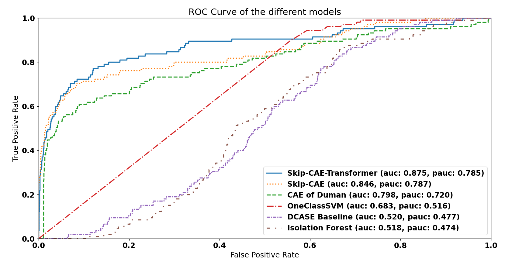
Figure 3: ROC curves, AUC and pAUC of the different models on the evaluation set

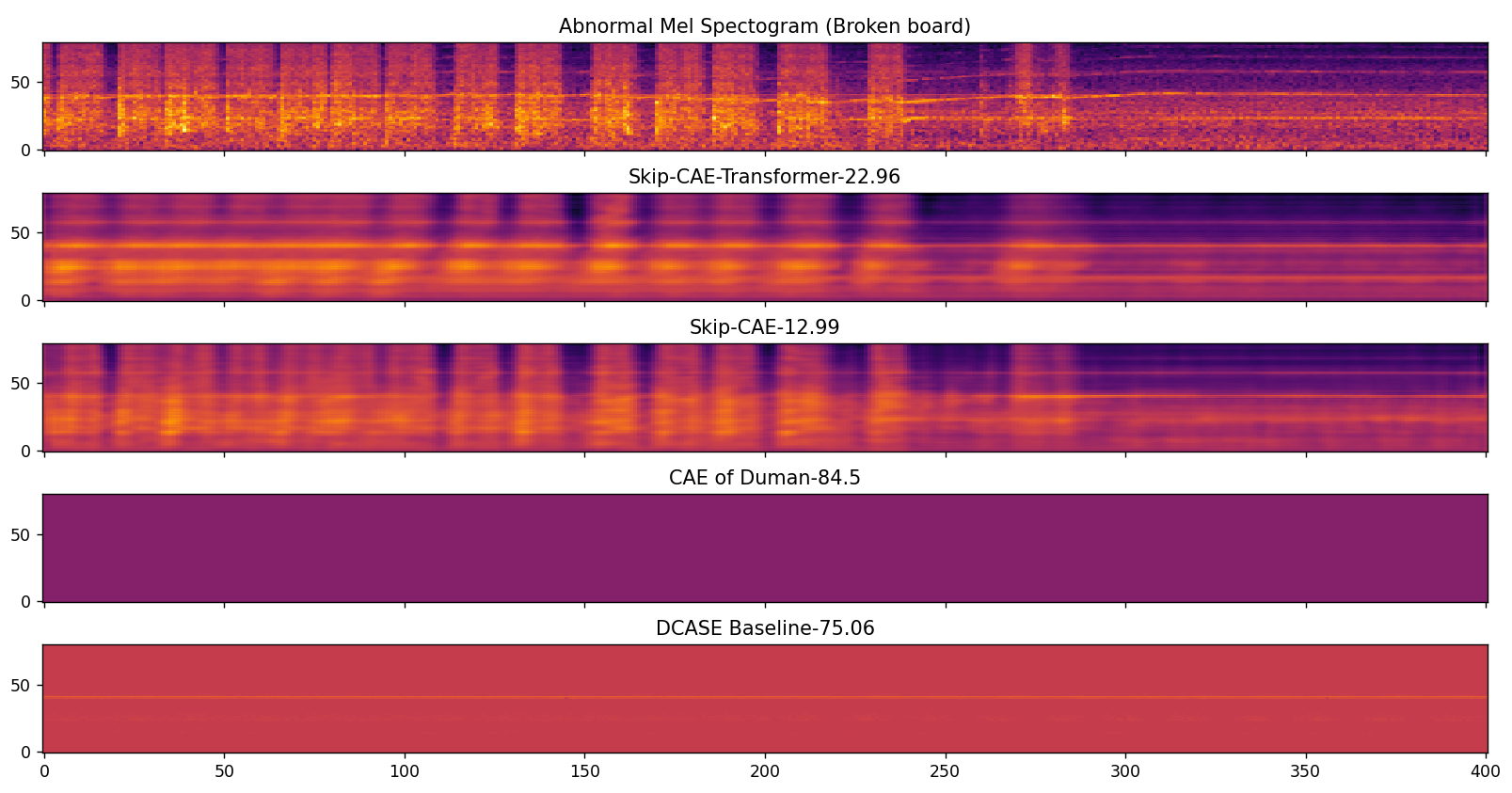
Figure 4: Mel spectogram of an anomaly (broken board) and the reconstructed mel spectograms of the neural network models with their reconstruction errors

V-B Results per anomaly type

Table II presents the AUC and pAUC of the different models for each type of anomaly. The best result for each metric is in bold. The CAE with skip connections and transformer (Skip-CAE-Transformer) outperforms all other models in AUC or pAUC for all of the anomaly types.

TABLE II: AUC and pAUC score of each model for each anomaly type

	Broken Board		Board Stuck		Uneven or Thick Wood
	AUC	pAUC	AUC	pAUC	AUC	pAUC
Skip-CAE-Transformer	0.743	0.677	0.778	0.744	0.921	0.807
Skip-CAE	0.777	0.618	0.723	0.729	0.900	0.820
CAE of Duman et al. [2]	0.757	0.644	0.639	0.676	0.864	0.742
OneClassSVM	0.558	0.509	0.707	0.519	0.681	0.515
DCASE Baseline	0.441	0.474	0.620	0.480	0.484	0.476
Isolation Forest	0.437	0.474	0.613	0.474	0.485	0.474

VI Conclusion

We developed two deep neural network models inspired by a CAE introduced by Duman et al. [2] to detect anomalies in audio signals from an industrial wood planer. The first model, Skip-CAE, is a CAE with skip connections to improve the convergence. The second, Skip-CAE-Transformer, has additional transformer encode and decode layers. For the experiments, we built a new public dataset of real-life-recorded wood planer operations containing 105 anomalies corresponding to stuck boards, broken boards and uneven or thick boards. We compared, on this dataset, the proposed neural networks to baselines such as one-class SVM, isolation forest, the CAE of Duman et al. [2], and a traditional autoencoder used in the DCASE 2024 challenge. Our best model, the Skip-CAE-Transformer, outperforms the other models obtaining an AUC of $0.875$. Grouping results by anomaly type reveals that the Skip-CAE-Transformer outperforms other models to detect stuck boards and uneven or thick wood. Our models thus demonstrate that it is feasible to detect abnormal events on industrial planers. Furthermore, acoustic anomaly detection is close to how operators function. As such, our models have the potential to gain the trust of expert operators who can understand their outcomes, but it can also help new operators understand the reason for the alarms/anomalies detected.

References

- [1] U. Buehlmann and R. E. Thomas, “Impact of human error on lumber yield in rough mills,” Robotics and Computer-Integrated Manufacturing, vol. 18, no. 3-4, pp. 197–203, 2002.
- [2] T. B. Duman, B. Bayram, and G. İnce, “Acoustic anomaly detection using convolutional autoencoders in industrial processes,” in 14th International Conference on Soft Computing Models in Industrial and Environmental Applications (SOCO 2019) Seville, Spain, May 13–15, 2019, Proceedings 14. Springer, 2020, pp. 432–442.
- [3] E. C. Nunes, “Anomalous sound detection with machine learning: A systematic review,” arXiv preprint arXiv:2102.07820, Feb. 2021.
- [4] A. Mohammadpanah, B. Lehmann, and J. White, “Development of a monitoring system for guided circular saws: an experimental investigation,” Wood Material Science & Engineering, vol. 14, no. 2, pp. 99–106, 2019.
- [5] M. Derbas, A. Jaquemod, S. Frömel-Frybort, K. Güzel, H.-C. Moehring, and M. Riegler, “Multisensor data fusion and machine learning to classify wood products and predict workpiece characteristics during milling,” CIRP Journal of Manufacturing Science and Technology, vol. 47, pp. 103–115, 2023.
- [6] J.-T. Sexton, M. Morin, R. Georges, F. Abasian, and J. Gaudreault, “Wood planer control: Predictive and prescriptive approaches via automatic state matching gaussian processes,” Engineering Applications of Artificial Intelligence, vol. 132, p. 107843, 2024.
- [7] M. Derbas, S. Frömel-Frybort, C. Laaber, H.-C. Möhring, and M. Riegler, “Supervised classification of wood species during milling based on extracted cut events from ultrasonic air-borne acoustic signals,” Wood Material Science & Engineering, vol. 18, no. 6, pp. 2040–2048, 2023.
- [8] V. Nasir, J. Cool, and F. Sassani, “Acoustic emission monitoring of sawing process: artificial intelligence approach for optimal sensory feature selection,” The International Journal of Advanced Manufacturing Technology, vol. 102, pp. 4179–4197, 2019.
- [9] R. Zhuo, Z. Deng, B. Chen, G. Liu, and S. Bi, “Overview on development of acoustic emission monitoring technology in sawing,” The International Journal of Advanced Manufacturing Technology, vol. 116, pp. 1411–1427, 2021.
- [10] P. Iskra and R. E. Hernández, “Toward a process monitoring of CNC wood router. Sensor selection and surface roughness prediction,” Wood Science and Technology, vol. 46, no. 1, pp. 115–128, Jan. 2012.
- [11] P. Iskra and C. Tanaka, “A comparison of selected acoustic signal analysis techniques to evaluate wood surface roughness produced during routing,” Wood Science and Technology, vol. 40, no. 3, pp. 247–259, Mar. 2006.
- [12] J.-T. Sexton, M. Morin, R. Georges, F. Abasian, and J. Gaudreault, “Automatic state matching gaussian process ensemble for wood planer control,” IFAC-PapersOnLine, vol. 55, no. 10, pp. 625–630, 2022.
- [13] A. R. Hilal, A. Sayedelahl, A. Tabibiazar, M. S. Kamel, and O. A. Basir, “A distributed sensor management for large-scale IoT indoor acoustic surveillance,” Future Generation Computer Systems, vol. 86, pp. 1170–1184, 2018.
- [14] Z. Mnasri, S. Rovetta, and F. Masulli, “Anomalous sound event detection: A survey of machine learning based methods and applications,” Multimedia Tools and Applications, vol. 81, no. 4, pp. 5537–5586, Feb. 2022.
- [15] Z. Li, R. Liu, and D. Wu, “Data-driven smart manufacturing: Tool wear monitoring with audio signals and machine learning,” Journal of Manufacturing Processes, vol. 48, pp. 66–76, Dec. 2019.
- [16] M. Antonini, M. Vecchio, F. Antonelli, P. Ducange, and C. Perera, “Smart audio sensors in the Internet of things edge for anomaly detection,” IEEE Access, vol. 6, pp. 67 594–67 610, 2018.
- [17] C. Cooper, J. Zhang, R. X. Gao, P. Wang, and I. Ragai, “Anomaly detection in milling tools using acoustic signals and generative adversarial networks,” Procedia Manufacturing, vol. 48, pp. 372–378, 2020.
- [18] Y. Tagawa, R. Maskeliūnas, and R. Damaševičius, “Acoustic anomaly detection of mechanical failures in noisy real-life factory environments,” Electronics, vol. 10, no. 19, p. 2329, 2021.
- [19] T. Nishida, N. Harada, D. Niizumi, D. Albertini, R. Sannino, S. Pradolini, F. Augusti, K. Imoto, K. Dohi, H. Purohit, T. Endo, and Y. Kawaguchi, “Description and discussion on DCASE 2024 challenge task 2: First-shot unsupervised anomalous sound detection for machine condition monitoring,” In arXiv e-prints: 2406.07250, 2024.
- [20] D. Y. Oh and I. D. Yun, “Residual error based anomaly detection using auto-encoder in SMD machine sound,” Sensors, vol. 18, no. 5, p. 1308, 2018.
- [21] N. Harada, D. Niizumi, D. Takeuchi, Y. Ohishi, and M. Yasuda, “First-shot anomaly detection for machine condition monitoring: A domain generalization baseline,” Proceedings of 31st European Signal Processing Conference (EUSIPCO), pp. 191–195, 2023.
- [22] A. Vaswani, N. Shazeer, N. Parmar, J. Uszkoreit, L. Jones, A. N. Gomez, Ł. Kaiser, and I. Polosukhin, “Attention is All you Need,” Advances in Neural Information Processing Systems, 2017.
- [23] I. Loshchilov and F. Hutter, “Decoupled weight decay regularization,” in International Conference on Learning Representations, 2019.
- [24] ——, “SGDR: Stochastic gradient descent with warm restarts,” in International Conference on Learning Representations, 2017. [Online]. Available: https://openreview.net/forum?id=Skq89Scxx
- [25] F. Pedregosa, G. Varoquaux, A. Gramfort, V. Michel, B. Thirion, O. Grisel, M. Blondel, P. Prettenhofer, R. Weiss, V. Dubourg, J. Vanderplas, A. Passos, D. Cournapeau, M. Brucher, M. Perrot, and E. Duchesnay, “Scikit-learn: Machine learning in Python,” Journal of Machine Learning Research, vol. 12, pp. 2825–2830, 2011.