The effect of finite mass in cavity-QED calculations
Abstract
The effect of finite nuclear mass is investigated in coupled light matter systems in cavity quantum electrodynamics (cavity QED) using the Pauli-Fierz Hamiltonian. Three different systems, the He atom, the H- ion and the H ion is investigated. There are small, but significant differences in the behavior of the binding energies as the function of the coupling strength. The probability of coupling to light is found to be very small but even this small coupling has a very strong effect on the energies of the systems.
I Introduction
Cavity quantum electrodynamics is a powerful platform for implementing quantum sensors [1, 2], memories[3, 4], and networks [5, 6, 7, 8, 9, 10]. In cavity QED, a quantum emitter, such as an atom, molecule or a quantum dot, is coupled to the electromagnetic modes confined within a cavity. Strong interactions between cavity photons and molecular systems can result in the formation of hybrid light-matter states called polaritons. These polaritons can exhibit significantly different chemical and physical properties compared to their individual components. The strongly coupled light-matter states can dramatically change physical and chemical processes. For example, a cavity can enhance the energy transport in molecules [11], suppress photochemical reactions [12], or induce catalytic processes [13, 14]. Cavities can also change reactivity [15, 16], photoisomerisation [17], ionization [18], excited states [19] or electron captures processes [20].
The ability to manipulate the physical and chemical characteristics of materials through interaction with light has sparked significant experimental [21, 22, 23, 24, 25, 26, 27, 28, 29, 30, 31, 32] and theoretical [33, 34, 35, 36, 37, 38, 39, 40, 41, 42, 43, 44, 45, 46, 47, 48, 49, 50, 51, 52, 53, 54, 55, 56, 57, 58, 59, 60, 61, 62, 63, 64, 61, 47, 65, 66, 67, 68, 69, 70, 71, 72, 73, 74, 75, 76, 77, 78, 79, 80, 81, 82, 83] interest. Several excellent review articles have been published, highlighting the current state of experimental and theoretical approaches related to light-matter interactions in cavities. These include reviews about the properties of hybrid light-matter states [84, 85], ab initio calculations [46, 86] and molecular polaritonics [87, 88, 89].
The theoretical and computational description of the coupled light-matter system is challenging because the already complex solution of the quantum many-body problem of the interaction between electrons and nuclei is further complicated by the addition of photon degrees of freedom. In recent years, a variety of approaches have been proposed that go beyond the simple two-level atom model [90]. Most of these approaches are based on successful many-body quantum methods adapted to the interaction with photons. The use of the Pauli-Fierz (PF) non-relativistic QED Hamiltonian has been found to be the most useful framework [46, 91, 50, 63, 71] for practical calculations. The PF Hamiltonian is a sum of electronic and photonic Hamiltonians, along with a cross-term describing the electron-photon interaction. Due to this cross term, one has to use a coupled electron-photon wave function,
| (1) |
where are the spatial coordinates of the electrons and nuclei and are the quantum numbers of the photon modes. The occupation number basis, , is used to represent the bosonic Fock-space of photon modes.
Wave function based approaches [92, 93, 94, 59, 95, 96, 97, 80, 81, 82, 83] typically use coupled electron-photon wave functions and the product form significally increases the dimensionality. The coupled cluster (CC) [94, 59, 95, 57] approach used in this context defines a reference wavefunction as a direct product of a Slater determinant of Hartree-Fock states and a zero-photon number state. The ground state QED-CC wavefunction is then obtained by applying an exponentiated cluster operator to this product state. The key benefit of this approach is its systematic improbability. Another approach, the recently introduced cavity quantum electrodynamics complete active space configuration method [97, 96, 98] uses linear combination of determinants of electronic orbitals and photon-number states to describe the system. Approaches using perturbation theory are also developed [99, 100, 83].
Density based approaches such as the quantum electrodynamics density functional theory (QEDFT) [60, 65, 66, 101, 102, 62, 103]. combine the very efficient density functional methods with the photon degrees of freedom. QEDFT is an exact reformulation of the PF Hamiltonian-based many-body wave theory. In practical QEDFT applications, one must develop good approximations of the fields and currents so that the auxiliary non-interacting system generates the same physical quantities as the interacting system. An alternative approach [104] uses a tensor product of real space density functional theory representation and photon-number states bringing the QEDFT closer to the wave function based approaches.
The PF Hamiltonian can be solved numerically exactly for a one electron atom or ion using product states of Gaussian basis functions and photon number states [105]. The properties of small atoms and molecules can also be accurately calculated by using a product state of correlated gaussian basis states [106] and photon number states [92, 93].
In this work, the stochastic variational method [107, 108, 92] will be used to optimize light-matter coupled wave functions. The calculations can reach the same accuracy as conventional high precision calculations for small system [92, 93].
The main aim of this work is to study the difference between the Born-Oppenheimer (infinite nuclear mass) and the non Born-Oppenheimer (finite nuclear mass) approaches. In most calculations [92, 93, 94, 59, 95, 80, 81, 82, 83] the nuclear masses assumed to be infinite and the nuclei are not treated quantum mechanically. The PF Hamiltonian, however, also contains a nuclei-photon coupling term and the dipole self-interaction (DSI) depend on the nuclear coordinates as well. This work will elucidate the role of these terms using small molecules and ions as test cases.
The spatial wave functions will be represented by Explicitly Correlated Gaussian (ECG) basis functions [106]. The advantage of the approach is that the matrix elements are analytically available [107, 109, 110] and it allows very accurate calculations of energies and wave functions [106, 111, 112, 113, 114, 115, 116].
II Formalism
II.1 Hamiltonian
The Hamiltonian of the system is
| (2) |
is the usual electronic Coulomb Hamiltonian, and is the electron photon interaction. The electron-photon interaction is described by using the PF nonrelativistic QED Hamiltonian. The PF Hamiltonian can be derived [46, 91, 50, 63, 71] by applying the Power-Zienau-Woolley gauge transformation [117], with a unitary phase transformation on the minimal coupling () Hamiltonian in the Coulomb gauge,
| (3) | |||||
where is the dipole operator. The photon fields are described by quantized oscillators. is the displacement field and is the conjugate momentum. This Hamiltonian describes photon modes with frequency and coupling . The coupling term is usually written as [101]
| (4) |
where is the mode function at position and is the transversal polarization vector of the photon modes. The three components of the electron-photon interaction are as follows: The photonic part is
| (5) |
and the interaction term is
| (6) |
The dipole self-interaction is defined as
| (7) |
and the importance of this term for the existence of a ground state is discussed in Ref. [91].
In the following, we will assume that there is only one important photon mode with frequency and coupling . Thus the suffix is omitted in what follows. The formalism can be easily extended for many photon modes but here we concentrate on calculating the matrix elements and it is sufficient to use a single-mode.
For one photon mode Eqs. (5), (6), and (7) can be simplified and the Hamiltonian becomes
| (8) |
In the following we assume that the system has particles with position , mass and charge . The position of the particles with infinite mass will be fixed at . The kinetic operator is
| (9) |
If the system only contains particles with finite mass, the kinetic energy operator can be rewritten as a sum of the kinetic energy operators of the relative and center of mass motion and the center of mass motion can be easily eliminated [107]. is the Coulomb interaction
| (10) |
is the nuclear potential in the case of fixed (infinite mass) nuclei
| (11) |
and the dipole moment of the system is defined as
| (12) |
The operators act in real space, except which acts on the photon space
II.2 Trial functions
Introducing the shorthand notations , and where is the number of photons in photon mode , the variational trial wave function is written as a linear combination of products of spatial and photon space basis functions
| (14) |
The spatial part of the wave function is expanded into ECGs for each photon state as
| (15) |
where is an antisymmetrizer, is the particle spin function (coupling the spin to ), and , and are nonlinear parameters.
The DSI introduces a non-spherical term into the Hamiltonian. The solution of this non-spherical problem is very difficult and slowly converging. To avoid this we introduce in Eq. (15) to eliminate the DSI term from Eq. (6) altogether. In the exponential, is a matrix with elements chosen in such a way that when the kinetic energy acts on the trial function, the resulting expression cancels the DSI term [92].
The necessary matrix elements can be analytically computed for both the spatial and the photon components [93, 92], and the resulting Hamiltonian and overlap matrices are highly sparse.
We will optimize the basis functions by selecting the best spatial basis parameters and photon components using the Stochastic Variational method (SVM) [107, 108]. In the SVM approach, a large number of candidate basis functions are randomly generated, and the ones that yield the lowest energy are chosen [92, 107, 108]. The basis size can be increased by adding the best states one by one, and a K-dimensional basis can be refined by replacing states with randomly selected better basis functions. This approach is very efficient in finding suitable basis functions.
III Results and discussion
Three systems, the and ions and the He atom is used as example. Atomic units will be used (=1, and =1) and the mass of the proton and the He nucleus is expressed in in electron mass . To calculate the binding energies we also have to calculate the energy of the H atom and He+ ion. The nuclei with infinite mass are positioned at the origin, except for the H ion the positions are and . For the coupling is chosen, and will be varied between and . The experimentally achievable value is somewhere below and most calculations use the 0.01-0.1 range. The basis size is 100 for one-particle cases (,H atom, H and He+ ions with infinite nuclear mass) 400 for two-particle cases (, H-, He with infinite mass) and 1000 for the three-particle systems. The nonlinear parameters are optimized until the energy converged in the first 6 decimals.
III.1 The H atom
| 0.01 | -0.499675 | -0.499691 | 0.999975 | 2.5 |
| 0.02 | -0.499521 | -0.499590 | 0.999900 | 1.0 |
| 0.03 | -0.499275 | -0.499421 | 0.999776 | 2.2 |
| 0.04 | -0.498925 | -0.499184 | 0.999605 | 3.9 |
| 0.05 | -0.498484 | -0.498883 | 0.999388 | 6.1 |
| 0.06 | -0.497933 | -0.498515 | 0.999120 | 8.7 |
| 0.07 | -0.497308 | -0.498071 | 0.998820 | 1.2 |
| 0.08 | -0.496585 | -0.497579 | 0.998468 | 1.5 |
| 0.09 | -0.495773 | -0.497014 | 0.998081 | 1.9 |
| 0.10 | -0.494873 | -0.496385 | 0.997660 | 2.3 |
Table 1 shows the energy of the H atom as a function of for the finite proton mass case. The first energy, , is the energy of the atom without coupling to photon spaces, the energy change in this case is purely due to the DSI term . The second energy, , in Table 1 is the energy of the system coupled to photon spaces , . We also show the probability of the wave function in the zero photon space () and the one photon space . As the DSI term is positive, the energy of the H atom increases with for both and . The probability of the photon space is small but increasing with . The probabilities of the higher photon spaces (not shown) are typically 10-3 times smaller, . These probabilities also increase with and for photon spaces up to contribute to the energy in the 5th or 6th decimals.
| 0.01 | -0.499932 | -0.499946 | 0.999976 | 2.4 |
| 0.02 | -0.499789 | -0.499844 | 0.999909 | 9.0 |
| 0.03 | -0.499542 | -0.499678 | 0.999793 | 2.1 |
| 0.04 | -0.499189 | -0.499447 | 0.999615 | 3.8 |
| 0.05 | -0.498737 | -0.499132 | 0.999386 | 6.1 |
| 0.06 | -0.498191 | -0.498783 | 0.999126 | 8.7 |
| 0.07 | -0.497569 | -0.498348 | 0.998824 | 1.2 |
| 0.08 | -0.496840 | -0.497850 | 0.998477 | 1.5 |
| 0.09 | -0.496027 | -0.497282 | 0.998095 | 1.9 |
| 0.10 | -0.495115 | -0.496655 | 0.997679 | 2.3 |
The infinite mass case (Table 2) shows very similar tendency, the photon space probabilities barely changed, the energies are slightly decreased due to the the increased mass.
III.2 The H- ion
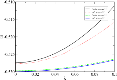
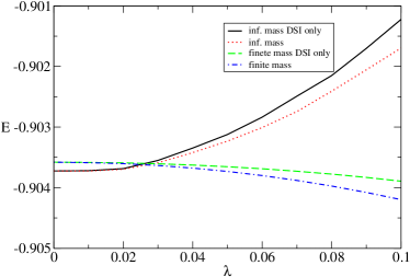
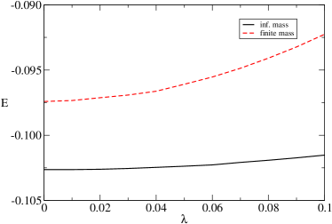
First, we show the calculation for the H- ion with finite proton mass. The effect of the cavity is much larger on the H- ion, as expected (see Table 3). This system is weakly bound, the dipole moment is larger and couples to the light much more strongly. The DSI ( column in Table 3) strongly increases the energy. The energy of the light-matter coupled system, , also increases with but not as strongly as . The coupling changes the energy in the second decimal and the probability of the zero photon space decreases to 0.95. The tendency is very similar for the infinite mass case but the energies are significantly different. This is illustrated in Fig. 1. The energy of the finite and infinite mass case changes to a different extent in the H- ion case, while in the case of the H atom the two energies change much less with and behave almost identically.
| 0.01 | -0.527025 | -0.527276 | 0.999152 | |
| 0.02 | -0.525849 | -0.526777 | 0.996681 | |
| 0.03 | -0.524030 | -0.525946 | 0.992822 | |
| 0.04 | -0.521667 | -0.524794 | 0.987690 | |
| 0.05 | -0.518830 | -0.523313 | 0.981802 | |
| 0.06 | -0.515572 | -0.521512 | 0.975452 | |
| 0.07 | -0.511936 | -0.519387 | 0.968746 | |
| 0.08 | -0.507957 | -0.516961 | 0.962100 | |
| 0.09 | -0.503653 | -0.514233 | 0.955476 | |
| 0.10 | -0.499061 | -0.511135 | 0.950017 |
| 0.01 | -0.527377 | -0.527632 | 0.999159 | |
| 0.02 | -0.526318 | -0.527268 | 0.996756 | |
| 0.03 | -0.524660 | -0.526551 | 0.993994 | |
| 0.04 | -0.522501 | -0.525778 | 0.988958 | |
| 0.05 | -0.520096 | -0.524732 | 0.983072 | |
| 0.06 | -0.517207 | -0.523379 | 0.980888 | |
| 0.07 | -0.514182 | -0.521570 | 0.975456 | |
| 0.08 | -0.510917 | -0.519876 | 0.966552 | |
| 0.09 | -0.507437 | -0.517978 | 0.961433 | |
| 0.10 | -0.503754 | -0.515700 | 0.956274 |
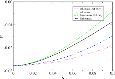
Fig. 2 shows the binding energy of the H- ion in the finite and infinite proton mass cases. The binding energy decreases as increases and the binding energy of the finite mass case decreases faster then the infinite one. The binding energy change due to the DSI alone behave similarly and the difference between the difference between the DSI total binding energy curves show the importance of the coupling to the light spaces.
III.3 The He atom
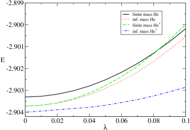
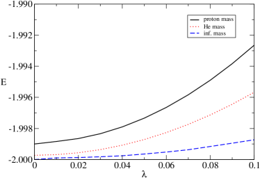
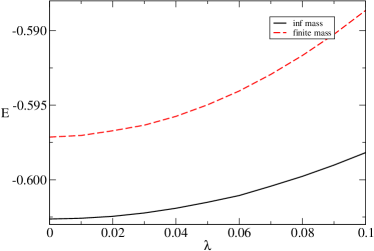
The energies of the He atom with finite and infinite nuclear mass are listed in Tables 5 and 6. Compared to the H- ion the electrons are strongly bound in the He atom and the energy change is much less when is increased. The photon space probabilities also remain very low about 10-4. The energy of the He atom and the He+ ion is also shown as the function of in Fig. 3. The energy curves of the finite and infinite mass He atom are very similar, but the dependence of the energy of finite and infinite mass He+ are significantly different. This is further investigated in Fig. 4, where we add a calculation using a smaller artificial mass (taken to be equal to the mass of a proton). Fig. 4 shows that the energy is increasing faster as the function of for lighter particles. This leads to a very interesting case for the binding energies shown in Fig. 5. The binding energy decreases with increasing for the infinite mass case, while the binding energy increases with increasing for the finite mass case. This is true for both the SDI and the full coupled Hamiltonian. As the binding energy of the infinite mass case is larger than the finite mass case there is a crossover at around .
| 0.00 | -2.903305 | -2.903305 | 1.0 | 0.0 |
| 0.01 | -2.903267 | -2.903273 | 0.999995 | 5.0 |
| 0.02 | -2.903153 | -2.903179 | 0.999980 | 2.0 |
| 0.03 | -2.902966 | -2.903022 | 0.999954 | 4.6 |
| 0.04 | -2.902703 | -2.902802 | 0.999919 | 8.1 |
| 0.05 | -2.902365 | -2.902510 | 0.999874 | 1.3 |
| 0.06 | -2.901953 | -2.902175 | 0.999820 | 1.8 |
| 0.07 | -2.901467 | -2.901768 | 0.999755 | 2.4 |
| 0.08 | -2.900907 | -2.901299 | 0.999685 | 3.2 |
| 0.09 | -2.900274 | -2.900768 | 0.999606 | 3.9 |
| 0.10 | -2.899569 | -2.900176 | 0.999527 | 4.7 |
| 0.00 | -2.903724 | -2.903724 | 1.0 | 0. |
| 0.01 | -2.903669 | -2.903677 | 0.999997 | 3.1 |
| 0.02 | -2.903556 | -2.903586 | 0.999984 | 1.6 |
| 0.03 | -2.903370 | -2.903422 | 0.999961 | 3.9 |
| 0.04 | -2.903102 | -2.903202 | 0.999924 | 7.5 |
| 0.05 | -2.902766 | -2.902915 | 0.999883 | 1.2 |
| 0.06 | -2.902354 | -2.902567 | 0.999834 | 1.7 |
| 0.07 | -2.901860 | -2.902168 | 0.999759 | 2.4 |
| 0.08 | -2.901310 | -2.901667 | 0.999710 | 2.9 |
| 0.09 | -2.900649 | -2.901123 | 0.999647 | 3.5 |
| 0.10 | -2.899953 | -2.900558 | 0.999512 | 4.8 |
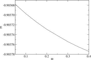
Finally, a note about the dependence on the cavity frequency. We have used in the calculations so far, but the results would barely change for different . As shown in Fig. 6 the change in the energy is very small for a wide range of , the binding energy only changes in the fifth digit.
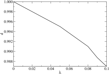
IV The H ion
The final example is the H molecular ion. In this case, for the infinite mass case we first calculated the equilibrium bond length as the function of and then fixed the distance between the two protons at the equilibrium and calculated the energy of the ion. As shown in Fig. 7 the bond length gets slightly lower with increasing . Figs. 8 and 9 shows the total energies and the binding energies of the finite and infinite mass cases as a function of . In this case, the energies behave very similarly except for an overall shift (the infinite mass case have larger total and binding energy), and the energy of the finite mass case changes somewhat more.
V Summary
The effect of finite nuclear mass is investigated in coupled light-matter systems in cavity QED using the Pauli-Fierz Hamiltonian. Three different systems are investigated: the helium atom, the hydrogen negative ion (H-), and the hydrogen molecular ion (H). The study finds small but significant differences in the behavior of the binding energies as a function of the coupling strength. The binding energy decreases for H and H- as increases for both finite and infinite mass in a similar way. For the He atom, however, the binding energy decreases for infinite mass and increases for finite mass. These differences are due to the competition of the kinetic energy terms and the dipole moment depending parts of the Hamiltonian. In the infinite mass case the nuclei are fixed and the nuclear coordinates do not contribute to the total dipole of the system. In the finite nuclear mass case the nuclear motion also effects the dipole moment and there is a balance between the kinetic energy of the nuclei and the nuclear dipole dependence of the PF Hamiltonian.
Additionally, the probability of coupling to light is found to be very small, but even this small coupling has a strong effect on the energies of the systems. For tightly bound systems like the H or He atoms 99% of the wave function is in the zero photon space for realistic values of . For weakly bound systems this probability drops to 95% and higher photons spaces become important as well.
These very accurate test calculations can serve as benchmark cases of QEDFT, QED-CC [94, 59, 95, 57] or configuration interaction [97, 96, 98] calculations. These calculations also show that the nuclear motion can be very important in cavity QED calculations. The infinite mass approximation can be corrected by the Born-Oppenheimer expansion in molecular calculations. Similar approach has been worked out for the cavity QED case [66]. The solution of the coupled nucleus-electron-photon case, however, is complicated.
Acknowledgements.
This work has been supported by the National Science Foundation (NSF) under Grant No. IRES 2245029 and DMR-2217759.Data Availability Statement
The data that support the findings of this study are available from the corresponding author upon reasonable request.
AUTHOR DECLARATIONS
Conflict of Interest
The authors have no conflict of interest to disclose.
References
- Degen, Reinhard, and Cappellaro [2017] C. Degen, F. Reinhard, and P. Cappellaro, “Quantum sensing,” Reviews of Modern Physics 89, 035002 (2017).
- Reiserer, Ritter, and Rempe [2013] A. Reiserer, S. Ritter, and G. Rempe, “Nondestructive Detection of an Optical Photon,” Science 342, 1349–1351 (2013).
- Specht et al. [2011] H. P. Specht, C. Nölleke, A. Reiserer, M. Uphoff, E. Figueroa, S. Ritter, and G. Rempe, “A single-atom quantum memory,” Nature 473, 190–193 (2011).
- Ma et al. [2022] L. Ma, X. Lei, J. Yan, R. Li, T. Chai, Z. Yan, X. Jia, C. Xie, and K. Peng, “High-performance cavity-enhanced quantum memory with warm atomic cell,” Nature Communications 13, 2368 (2022).
- Reiserer and Rempe [2015] A. Reiserer and G. Rempe, “Cavity-based quantum networks with single atoms and optical photons,” Reviews of Modern Physics 87, 1379–1418 (2015).
- Daiss et al. [2021] S. Daiss, S. Langenfeld, S. Welte, E. Distante, P. Thomas, L. Hartung, O. Morin, and G. Rempe, “A quantum-logic gate between distant quantum-network modules,” Science 371, 614–617 (2021).
- Boozer et al. [2007] A. D. Boozer, A. Boca, R. Miller, T. E. Northup, and H. J. Kimble, “Reversible State Transfer between Light and a Single Trapped Atom,” Physical Review Letters 98, 193601 (2007).
- Ritter et al. [2012] S. Ritter, C. Nölleke, C. Hahn, A. Reiserer, A. Neuzner, M. Uphoff, M. Mücke, E. Figueroa, J. Bochmann, and G. Rempe, “An elementary quantum network of single atoms in optical cavities,” Nature 484, 195–200 (2012).
- Briegel et al. [1998] H.-J. Briegel, W. Dür, J. I. Cirac, and P. Zoller, “Quantum Repeaters: The Role of Imperfect Local Operations in Quantum Communication,” Physical Review Letters 81, 5932–5935 (1998).
- Muralidharan et al. [2016] S. Muralidharan, L. Li, J. Kim, N. Lütkenhaus, M. D. Lukin, and L. Jiang, “Optimal architectures for long distance quantum communication,” Scientific Reports 6, 20463 (2016).
- Sandik et al. [2024] G. Sandik, J. Feist, F. J. García-Vidal, and T. Schwartz, “Cavity-enhanced energy transport in molecular systems,” Nature Materials (2024), 10.1038/s41563-024-01962-5.
- Galego, Garcia-Vidal, and Feist [2016a] J. Galego, F. J. Garcia-Vidal, and J. Feist, “Suppressing photochemical reactions with quantized light fields,” Nature Communications 7, 13841 (2016a).
- Campos-Gonzalez-Angulo, Ribeiro, and Yuen-Zhou [2019] J. A. Campos-Gonzalez-Angulo, R. F. Ribeiro, and J. Yuen-Zhou, “Resonant catalysis of thermally activated chemical reactions with vibrational polaritons,” Nature Communications 10, 4685 (2019).
- Lather et al. [2019] J. Lather, P. Bhatt, A. Thomas, T. W. Ebbesen, and J. George, “Cavity Catalysis by Cooperative Vibrational Strong Coupling of Reactant and Solvent Molecules,” Angewandte Chemie International Edition 58, 10635–10638 (2019).
- Galego et al. [2019] J. Galego, C. Climent, F. J. Garcia-Vidal, and J. Feist, “Cavity Casimir-Polder Forces and Their Effects in Ground-State Chemical Reactivity,” Physical Review X 9, 021057 (2019).
- Thomas et al. [2019a] A. Thomas, L. Lethuillier-Karl, K. Nagarajan, R. M. A. Vergauwe, J. George, T. Chervy, A. Shalabney, E. Devaux, C. Genet, J. Moran, and T. W. Ebbesen, “Tilting a ground-state reactivity landscape by vibrational strong coupling,” Science 363, 615–619 (2019a).
- Fregoni et al. [2018] J. Fregoni, G. Granucci, E. Coccia, M. Persico, and S. Corni, “Manipulating azobenzene photoisomerization through strong light–molecule coupling,” Nature Communications 9, 4688 (2018).
- Li, Nitzan, and Subotnik [2021] T. E. Li, A. Nitzan, and J. E. Subotnik, “Collective Vibrational Strong Coupling Effects on Molecular Vibrational Relaxation and Energy Transfer: Numerical Insights via Cavity Molecular Dynamics Simulations,” Angewandte Chemie International Edition 60, 15533–15540 (2021).
- Stranius, Hertzog, and Börjesson [2018] K. Stranius, M. Hertzog, and K. Börjesson, “Selective manipulation of electronically excited states through strong light–matter interactions,” Nature Communications 9, 2273 (2018).
- Cederbaum and Fedyk [2024] L. S. Cederbaum and J. Fedyk, “Making molecules in cavity,” The Journal of Chemical Physics 161, 074303 (2024).
- Hutchison et al. [2012] J. A. Hutchison, T. Schwartz, C. Genet, E. Devaux, and T. W. Ebbesen, “Modifying chemical landscapes by coupling to vacuum fields,” Angewandte Chemie International Edition 51, 1592–1596 (2012), https://onlinelibrary.wiley.com/doi/pdf/10.1002/anie.201107033 .
- Balili et al. [2007] R. Balili, V. Hartwell, D. Snoke, L. Pfeiffer, and K. West, “Bose-einstein condensation of microcavity polaritons in a trap,” Science 316, 1007–1010 (2007), https://science.sciencemag.org/content/316/5827/1007.full.pdf .
- Schachenmayer et al. [2015] J. Schachenmayer, C. Genes, E. Tignone, and G. Pupillo, “Cavity-enhanced transport of excitons,” Phys. Rev. Lett. 114, 196403 (2015).
- Xiang et al. [2020] B. Xiang, R. F. Ribeiro, M. Du, L. Chen, Z. Yang, J. Wang, J. Yuen-Zhou, and W. Xiong, “Intermolecular vibrational energy transfer enabled by microcavity strong light–matter coupling,” Science 368, 665–667 (2020), https://science.sciencemag.org/content/368/6491/665.full.pdf .
- Reserbat-Plantey et al. [2021] A. Reserbat-Plantey, I. Epstein, I. Torre, A. T. Costa, P. A. D. Gonçalves, N. A. Mortensen, M. Polini, J. C. W. Song, N. M. R. Peres, and F. H. L. Koppens, “Quantum nanophotonics in two-dimensional materials,” ACS Photonics 8, 85–101 (2021).
- Coles et al. [2014] D. M. Coles, N. Somaschi, P. Michetti, C. Clark, P. G. Lagoudakis, P. G. Savvidis, and D. G. Lidzey, “Polariton-mediated energy transfer between organic dyes in a strongly coupled optical microcavity,” Nature Materials 13, 712–719 (2014).
- Kasprzak et al. [2006] J. Kasprzak, M. Richard, S. Kundermann, A. Baas, P. Jeambrun, J. M. J. Keeling, F. M. Marchetti, M. H. Szymańska, R. André, J. L. Staehli, V. Savona, P. B. Littlewood, B. Deveaud, and L. S. Dang, “Bose–einstein condensation of exciton polaritons,” Nature 443, 409–414 (2006).
- Schwartz et al. [2011] T. Schwartz, J. A. Hutchison, C. Genet, and T. W. Ebbesen, “Reversible switching of ultrastrong light-molecule coupling,” Phys. Rev. Lett. 106, 196405 (2011).
- Plumhof et al. [2014] J. D. Plumhof, T. Stöferle, L. Mai, U. Scherf, and R. F. Mahrt, “Room-temperature bose–einstein condensation of cavity exciton–polaritons in a polymer,” Nature Materials 13, 247–252 (2014).
- Hutchison et al. [2013] J. A. Hutchison, A. Liscio, T. Schwartz, A. Canaguier-Durand, C. Genet, V. Palermo, P. Samorì, and T. W. Ebbesen, “Tuning the work-function via strong coupling,” Advanced Materials 25, 2481–2485 (2013), https://onlinelibrary.wiley.com/doi/pdf/10.1002/adma.201203682 .
- Wang et al. [2021a] K. Wang, M. Seidel, K. Nagarajan, T. Chervy, C. Genet, and T. Ebbesen, “Large optical nonlinearity enhancement under electronic strong coupling,” Nature Communications 12, 1486 (2021a).
- Basov et al. [2021] D. N. Basov, A. Asenjo-Garcia, P. J. Schuck, X. Zhu, and A. Rubio, “Polariton panorama,” Nanophotonics 10, 549–577 (2021).
- Feist and Garcia-Vidal [2015] J. Feist and F. J. Garcia-Vidal, “Extraordinary exciton conductance induced by strong coupling,” Phys. Rev. Lett. 114, 196402 (2015).
- Vendrell [2018] O. Vendrell, “Collective jahn-teller interactions through light-matter coupling in a cavity,” Phys. Rev. Lett. 121, 253001 (2018).
- Schäfer and Johansson [2022] C. Schäfer and G. Johansson, “Shortcut to self-consistent light-matter interaction and realistic spectra from first principles,” Phys. Rev. Lett. 128, 156402 (2022).
- Riso et al. [2022] R. R. Riso, T. S. Haugland, E. Ronca, and H. Koch, “Molecular orbital theory in cavity qed environments,” Nature Communications 13, 1368 (2022).
- Badankó et al. [2022] P. Badankó, O. Umarov, C. Fb́ri, G. J. Halász, and A. Vibók, “Topological aspects of cavity-induced degeneracies in polyatomic molecules,” International Journal of Quantum Chemistry 122, e26750 (2022), https://onlinelibrary.wiley.com/doi/pdf/10.1002/qua.26750 .
- Mazza and Georges [2019] G. Mazza and A. Georges, “Superradiant quantum materials,” Phys. Rev. Lett. 122, 017401 (2019).
- Di Stefano et al. [2019] O. Di Stefano, A. Settineri, V. Macrì, L. Garziano, R. Stassi, S. Savasta, and F. Nori, “Resolution of gauge ambiguities in ultrastrong-coupling cavity quantum electrodynamics,” Nature Physics 15, 803–808 (2019).
- Galego, Garcia-Vidal, and Feist [2015] J. Galego, F. J. Garcia-Vidal, and J. Feist, “Cavity-induced modifications of molecular structure in the strong-coupling regime,” Phys. Rev. X 5, 041022 (2015).
- Herrera and Spano [2016] F. Herrera and F. C. Spano, “Cavity-controlled chemistry in molecular ensembles,” Phys. Rev. Lett. 116, 238301 (2016).
- Galego, Garcia-Vidal, and Feist [2016b] J. Galego, F. J. Garcia-Vidal, and J. Feist, “Suppressing photochemical reactions with quantized light fields,” Nature Communications 7, 13841 (2016b).
- Shalabney et al. [2015] A. Shalabney, J. George, J. Hutchison, G. Pupillo, C. Genet, and T. W. Ebbesen, “Coherent coupling of molecular resonators with a microcavity mode,” Nature Communications 6, 5981 (2015).
- Buchholz et al. [2019] F. Buchholz, I. Theophilou, S. E. B. Nielsen, M. Ruggenthaler, and A. Rubio, “Reduced density-matrix approach to strong matter-photon interaction,” ACS Photonics 6, 2694–2711 (2019).
- Schäfer et al. [2019] C. Schäfer, M. Ruggenthaler, H. Appel, and A. Rubio, “Modification of excitation and charge transfer in cavity quantum-electrodynamical chemistry,” Proceedings of the National Academy of Sciences 116, 4883–4892 (2019), https://www.pnas.org/content/116/11/4883.full.pdf .
- Ruggenthaler et al. [2018] M. Ruggenthaler, N. Tancogne-Dejean, J. Flick, H. Appel, and A. Rubio, “From a quantum-electrodynamical light–matter description to novel spectroscopies,” Nature Reviews Chemistry 2, 0118 (2018).
- Flick et al. [2015] J. Flick, M. Ruggenthaler, H. Appel, and A. Rubio, “Kohn–sham approach to quantum electrodynamical density-functional theory: Exact time-dependent effective potentials in real space,” Proceedings of the National Academy of Sciences 112, 15285–15290 (2015), https://www.pnas.org/content/112/50/15285.full.pdf .
- Flick et al. [2017] J. Flick, M. Ruggenthaler, H. Appel, and A. Rubio, “Atoms and molecules in cavities, from weak to strong coupling in quantum-electrodynamics (qed) chemistry,” Proceedings of the National Academy of Sciences 114, 3026–3034 (2017), https://www.pnas.org/content/114/12/3026.full.pdf .
- Lacombe, Hoffmann, and Maitra [2019] L. Lacombe, N. M. Hoffmann, and N. T. Maitra, “Exact potential energy surface for molecules in cavities,” Phys. Rev. Lett. 123, 083201 (2019).
- Mandal, Montillo Vega, and Huo [2020] A. Mandal, S. Montillo Vega, and P. Huo, “Polarized fock states and the dynamical casimir effect in molecular cavity quantum electrodynamics,” The Journal of Physical Chemistry Letters 11, 9215–9223 (2020), pMID: 32991814.
- Flick et al. [2019] J. Flick, D. M. Welakuh, M. Ruggenthaler, H. Appel, and A. Rubio, “Light–matter response in nonrelativistic quantum electrodynamics,” ACS Photonics 6, 2757–2778 (2019).
- Latini et al. [2019] S. Latini, E. Ronca, U. De Giovannini, H. Hübener, and A. Rubio, “Cavity control of excitons in two-dimensional materials,” Nano Letters 19, 3473–3479 (2019), pMID: 31046291.
- Flick, Rivera, and Narang [2018] J. Flick, N. Rivera, and P. Narang, “Strong light-matter coupling in quantum chemistry and quantum photonics,” Nanophotonics 7, 1479–1501 (2018).
- Flick and Narang [2018] J. Flick and P. Narang, “Cavity-correlated electron-nuclear dynamics from first principles,” Phys. Rev. Lett. 121, 113002 (2018).
- Garcia-Vidal, Ciuti, and Ebbesen [2021] F. J. Garcia-Vidal, C. Ciuti, and T. W. Ebbesen, “Manipulating matter by strong coupling to vacuum fields,” Science 373 (2021), 10.1126/science.abd0336, https://science.sciencemag.org/content/373/6551/eabd0336.full.pdf .
- Thomas et al. [2019b] A. Thomas, L. Lethuillier-Karl, K. Nagarajan, R. M. A. Vergauwe, J. George, T. Chervy, A. Shalabney, E. Devaux, C. Genet, J. Moran, and T. W. Ebbesen, “Tilting a ground-state reactivity landscape by vibrational strong coupling,” Science 363, 615–619 (2019b), https://science.sciencemag.org/content/363/6427/615.full.pdf .
- Mordovina et al. [2020] U. Mordovina, C. Bungey, H. Appel, P. J. Knowles, A. Rubio, and F. R. Manby, “Polaritonic coupled-cluster theory,” Phys. Rev. Research 2, 023262 (2020).
- Wang et al. [2021b] D. S. Wang, T. Neuman, J. Flick, and P. Narang, “Light–matter interaction of a molecule in a dissipative cavity from first principles,” The Journal of Chemical Physics 154, 104109 (2021b).
- DePrince [2021] A. E. DePrince, “Cavity-modulated ionization potentials and electron affinities from quantum electrodynamics coupled-cluster theory,” The Journal of Chemical Physics 154, 094112 (2021).
- Haugland et al. [2021] T. S. Haugland, C. Schäfer, E. Ronca, A. Rubio, and H. Koch, “Intermolecular interactions in optical cavities: An ab initio qed study,” The Journal of Chemical Physics 154, 094113 (2021).
- Hoffmann et al. [2020] N. M. Hoffmann, L. Lacombe, A. Rubio, and N. T. Maitra, “Effect of many modes on self-polarization and photochemical suppression in cavities,” The Journal of Chemical Physics 153, 104103 (2020).
- Flick and Narang [2020] J. Flick and P. Narang, “Ab initio polaritonic potential-energy surfaces for excited-state nanophotonics and polaritonic chemistry,” The Journal of Chemical Physics 153, 094116 (2020).
- Mandal, Krauss, and Huo [2020] A. Mandal, T. D. Krauss, and P. Huo, “Polariton-mediated electron transfer via cavity quantum electrodynamics,” The Journal of Physical Chemistry B 124, 6321–6340 (2020), pMID: 32589846.
- Galego, Garcia-Vidal, and Feist [2017] J. Galego, F. J. Garcia-Vidal, and J. Feist, “Many-molecule reaction triggered by a single photon in polaritonic chemistry,” Phys. Rev. Lett. 119, 136001 (2017).
- Flick et al. [2018] J. Flick, C. Schäfer, M. Ruggenthaler, H. Appel, and A. Rubio, “Ab initio optimized effective potentials for real molecules in optical cavities: Photon contributions to the molecular ground state,” ACS Photonics 5, 992–1005 (2018).
- Schafer, Ruggenthaler, and Rubio [2018] C. Schafer, M. Ruggenthaler, and A. Rubio, “Ab initio nonrelativistic quantum electrodynamics: Bridging quantum chemistry and quantum optics from weak to strong coupling,” Phys. Rev. A 98, 043801 (2018).
- Sidler et al. [2020] D. Sidler, M. Ruggenthaler, H. Appel, and A. Rubio, “Chemistry in quantum cavities: Exact results, the impact of thermal velocities, and modified dissociation,” The Journal of Physical Chemistry Letters 11, 7525–7530 (2020), pMID: 32805122.
- Theophilou et al. [2020] I. Theophilou, M. Penz, M. Ruggenthaler, and A. Rubio, “Virial relations for electrons coupled to quantum field modes,” Journal of Chemical Theory and Computation 16, 6236–6243 (2020), pMID: 32816479.
- Sidler et al. [2021] D. Sidler, C. Schäfer, M. Ruggenthaler, and A. Rubio, “Polaritonic chemistry: Collective strong coupling implies strong local modification of chemical properties,” The Journal of Physical Chemistry Letters 12, 508–516 (2021), pMID: 33373238.
- Buchholz et al. [2020] F. Buchholz, I. Theophilou, K. J. H. Giesbertz, M. Ruggenthaler, and A. Rubio, “Light–matter hybrid-orbital-based first-principles methods: The influence of polariton statistics,” Journal of Chemical Theory and Computation 16, 5601–5620 (2020), pMID: 32692551.
- Tokatly [2018] I. V. Tokatly, “Conserving approximations in cavity quantum electrodynamics: Implications for density functional theory of electron-photon systems,” Phys. Rev. B 98, 235123 (2018).
- Rivera, Flick, and Narang [2019] N. Rivera, J. Flick, and P. Narang, “Variational theory of nonrelativistic quantum electrodynamics,” Phys. Rev. Lett. 122, 193603 (2019).
- Szidarovszky, Halász, and Vibók [2020] T. Szidarovszky, G. J. Halász, and Á. Vibók, “Three-player polaritons: nonadiabatic fingerprints in an entangled atom–molecule–photon system,” New Journal of Physics 22, 053001 (2020).
- Cederbaum [2021] L. S. Cederbaum, “Polaritonic states of matter in a rotating cavity,” The Journal of Physical Chemistry Letters 12, 6056–6061 (2021), pMID: 34165990.
- Cho, Gu, and Mukamel [2022] D. Cho, B. Gu, and S. Mukamel, “Optical cavity manipulation and nonlinear uv molecular spectroscopy of conical intersections in pyrazine,” Journal of the American Chemical Society 144, 7758–7767 (2022), pMID: 35404593.
- Pavosevic and Rubio [0] F. Pavosevic and A. Rubio, “Wavefunction embedding for molecular polaritons,” The Journal of Chemical Physics 0, null (0).
- Pavošević and Flick [2021] F. Pavošević and J. Flick, “Polaritonic unitary coupled cluster for quantum computations,” The Journal of Physical Chemistry Letters 12, 9100–9107 (2021), pMID: 34520211.
- Pavošević et al. [2022] F. Pavošević, S. Hammes-Schiffer, A. Rubio, and J. Flick, “Cavity-modulated proton transfer reactions,” Journal of the American Chemical Society 144, 4995–5002 (2022), pMID: 35271261.
- Cederbaum and Kuleff [2021] L. S. Cederbaum and A. I. Kuleff, “Impact of cavity on interatomic coulombic decay,” Nature Communications 12, 4083 (2021).
- Bauer and Dreuw [2023a] M. Bauer and A. Dreuw, “Perturbation theoretical approaches to strong light–matter coupling in ground and excited electroni c states for the description of molecular polaritons,” The Journal of Chemical Physics 158, 124128 (2023a).
- Lexander et al. [2024] M. T. Lexander, S. Angelico, E. F. Kjønstad, and H. Koch, “Analytical evaluation of ground state gradients in quantum electrodynamics coupled cluster theory,” Journal of Chemical Theory and Computation 20, 8876–8885 (2024).
- Liebenthal and DePrince [2024] M. D. Liebenthal and I. DePrince, A. Eugene, “The orientation dependence of cavity-modified chemistry,” The Journal of Chemical Physics 161, 064109 (2024).
- Cui, Mandal, and Reichman [2024] Z.-H. Cui, A. Mandal, and D. R. Reichman, “Variational lang–firsov approach plus møller–plesset perturbation theory with applications to ab initio polariton chemistry,” Journal of Chemical Theory and Computation 20, 1143–1156 (2024).
- Ebbesen [2016] T. W. Ebbesen, “Hybrid light–matter states in a molecular and material science perspective,” Accounts of Chemical Research 49, 2403–2412 (2016).
- Genet, Faist, and Ebbesen [2021] C. Genet, J. Faist, and T. W. Ebbesen, “Inducing new material properties with hybrid light–matter states,” Physics Today 74, 42–48 (2021).
- Sidler et al. [2022] D. Sidler, M. Ruggenthaler, C. Schäfer, E. Ronca, and A. Rubio, “A perspective on ab initio modeling of polaritonic chemistry: The role of non-equilibrium effects and quantum collectivity,” The Journal of Chemical Physics 156, 230901 (2022).
- Li et al. [2022] T. E. Li, B. Cui, J. E. Subotnik, and A. Nitzan, “Molecular polaritonics: Chemical dynamics under strong light–matter coupling,” Annual Review of Physical Chemistry 73, 43–71 (2022).
- Sánchez-Barquilla et al. [2022] M. Sánchez-Barquilla, A. I. Fernández-Domínguez, J. Feist, and F. J. García-Vidal, “A theoretical perspective on molecular polaritonics,” ACS Photonics 9, 1830–1841 (2022).
- Fregoni, Garcia-Vidal, and Feist [2022] J. Fregoni, F. J. Garcia-Vidal, and J. Feist, “Theoretical challenges in polaritonic chemistry,” ACS Photonics 9, 1096–1107 (2022).
- Jaynes and Cummings [1962] E. Jaynes and F. W. Cummings, “Comparison of quantum and semiclassical radiation theories with application to the beam maser,” (1962).
- Rokaj et al. [2018] V. Rokaj, D. M. Welakuh, M. Ruggenthaler, and A. Rubio, “Light–matter interaction in the long-wavelength limit: no ground-state without dipole self-energy,” Journal of Physics B: Atomic, Molecular and Optical Physics 51, 034005 (2018).
- Ahrens et al. [2021] A. Ahrens, C. Huang, M. Beutel, C. Covington, and K. Varga, “Stochastic variational approach to small atoms and molecules coupled to quantum field modes in cavity qed,” Phys. Rev. Lett. 127, 273601 (2021).
- Beutel et al. [2021] M. Beutel, A. Ahrens, C. Huang, Y. Suzuki, and K. Varga, “Deformed explicitly correlated gaussians,” The Journal of Chemical Physics 155, 214103 (2021).
- Liebenthal, Vu, and DePrince [2022] M. D. Liebenthal, N. Vu, and A. E. DePrince, “Equation-of-motion cavity quantum electrodynamics coupled-cluster theory for electron attachment,” The Journal of Chemical Physics 156, 054105 (2022).
- Haugland et al. [2020] T. S. Haugland, E. Ronca, E. F. Kjønstad, A. Rubio, and H. Koch, “Coupled cluster theory for molecular polaritons: Changing ground and excited states,” Phys. Rev. X 10, 041043 (2020).
- Manderna, Vu, and Foley [2024] R. Manderna, N. Vu, and I. Foley, Jonathan J., “Comparing parameterized and self-consistent approaches to ab initio cavity quantum electrodynamics for electronic strong coupling,” The Journal of Chemical Physics 161, 174105 (2024), https://pubs.aip.org/aip/jcp/article-pdf/doi/10.1063/5.0230565/20228799/174105_1_5.0230565.pdf .
- Vu et al. [2024] N. Vu, D. Mejia-Rodriguez, N. P. Bauman, A. Panyala, E. Mutlu, N. Gov ind, and J. J. I. Foley, “Cavity quantum electrodynamics complete active space configuration interaction theory,” Journal of Chemical Theory and Computation 20, 1214–1227 (2024), pMID: 38291561.
- Matoušek et al. [2024] M. Matoušek, N. Vu, N. Govind, J. J. I. Foley, and L. Veis, “Polaritonic Chemistry Using the Density Matrix Renormalization Group Method,” Journal of Chemical Theory and Computation 20, 9424–9434 (2024).
- Bauer and Dreuw [2023b] M. Bauer and A. Dreuw, “Perturbation theoretical approaches to strong light–matter coupling in ground and excited electronic states for the description of molecular polaritons,” The Journal of Chemical Physics 158, 124128 (2023b).
- Szidarovszky [2023] T. Szidarovszky, “An efficient and flexible approach for computing rovibrational polaritons from first principles,” The Journal of Chemical Physics 159, 014112 (2023).
- Ruggenthaler et al. [2014] M. Ruggenthaler, J. Flick, C. Pellegrini, H. Appel, I. V. Tokatly, and A. Rubio, “Quantum-electrodynamical density-functional theory: Bridging quantum optics and electronic-structure theory,” Phys. Rev. A 90, 012508 (2014).
- Tokatly [2013] I. V. Tokatly, “Time-dependent density functional theory for many-electron systems interacting with cavity photons,” Phys. Rev. Lett. 110, 233001 (2013).
- Yang et al. [2021] J. Yang, Q. Ou, Z. Pei, H. Wang, B. Weng, Z. Shuai, K. Mullen, and Y. Shao, “Quantum-electrodynamical time-dependent density functional theory within gaussian atomic basis,” The Journal of Chemical Physics 155, 064107 (2021).
- Malave et al. [2022] J. Malave, A. Ahrens, D. Pitagora, C. Covington, and K. Varga, “Real-space, real-time approach to quantum-electrodynamical time-dependent d ensity functional theory,” The Journal of Chemical Physics 157, 194106 (2022).
- Aklilu and Varga [2024] Y. S. Aklilu and K. Varga, “Description of the hydrogen atom and the ion in an optical cavity using the pauli-fierz hamiltonian,” Phys. Rev. A 110, 043119 (2024).
- Mitroy et al. [2013] J. Mitroy, S. Bubin, W. Horiuchi, Y. Suzuki, L. Adamowicz, W. Cencek, K. Szalewicz, J. Komasa, D. Blume, and K. Varga, “Theory and application of explicitly correlated gaussians,” Rev. Mod. Phys. 85, 693–749 (2013).
- Suzuki, , and Varga [1998] Y. Suzuki, , and K. Varga, Stochastic variational approach to quantum-mechanical few-body problems, Vol. 54 (Springer Science & Business Media, 1998).
- Varga and Suzuki [1995] K. Varga and Y. Suzuki, “Precise solution of few-body problems with the stochastic variational method on a correlated gaussian basis,” Phys. Rev. C 52, 2885–2905 (1995).
- Cioslowski and Strasburger [2017] J. Cioslowski and K. Strasburger, “Harmonium atoms at weak confinements: The formation of the wigner molecules,” The Journal of Chemical Physics 146, 044308 (2017).
- Zaklama et al. [2019] T. Zaklama, D. Zhang, K. Rowan, L. Schatzki, Y. Suzuki, and K. Varga, “Matrix elements of one dimensional explicitly correlated gaussian basis functions,” Few-Body Systems 61, 6 (2019).
- Zhang, Kidd, and Varga [2015] D. K. Zhang, D. W. Kidd, and K. Varga, “Excited biexcitons in transition metal dichalcogenides,” Nano Letters 15, 7002–7005 (2015).
- Kidd, Zhang, and Varga [2016] D. W. Kidd, D. K. Zhang, and K. Varga, “Binding energies and structures of two-dimensional excitonic complexes in transition metal dichalcogenides,” Phys. Rev. B 93, 125423 (2016).
- Riva, Peeters, and Varga [2000] C. Riva, F. M. Peeters, and K. Varga, “Excitons and charged excitons in semiconductor quantum wells,” Phys. Rev. B 61, 13873–13881 (2000).
- Varga [1999] K. Varga, “Multipositronic systems,” Phys. Rev. Lett. 83, 5471–5474 (1999).
- Usukura, Suzuki, and Varga [1999] J. Usukura, Y. Suzuki, and K. Varga, “Stability of two- and three-dimensional excitonic complexes,” Phys. Rev. B 59, 5652–5661 (1999).
- Varga et al. [2001] K. Varga, P. Navratil, J. Usukura, and Y. Suzuki, “Stochastic variational approach to few-electron artificial atoms,” Phys. Rev. B 63, 205308 (2001).
- Power, Zienau, and Massey [1959] E. A. Power, S. Zienau, and H. S. W. Massey, “Coulomb gauge in non-relativistic quantum electro-dynamics and the shape of spectral lines,” Philosophical Transactions of the Royal Society of London. Series A, Mathematical and Physical Sciences 251, 427–454 (1959), https://royalsocietypublishing.org/doi/pdf/10.1098/rsta.1959.0008 .