Kinematics Calibration and Excitation Energy Reconstruction for Solenoidal Spectrometers

Abstract

Solenoidal spectrometers are gaining popularity worldwide due to their large acceptance and superior Q-value resolution in reactions involving radioactive beams. This work introduces a novel recoil energy calibration method leveraging known excited states. Building on this calibration, we describe an algorithm that transforms energy-position data into excitation energy and center-of-mass. This approach has been integrated into the HELIOS online analysis routines, enabling the real-time and speedy generation of excitation energy spectra and angular distributions during experiments.

1 Introduction

Solenoidal spectrometers [1] are specialized devices used in nuclear reactions such as A($a$, $b$)B, where only particle B can be excited. These spectrometers transform the excitation energy of particle B ($E_{x}$ in MeV) and the center-of-mass scattering angle ($\theta_{cm}$) into the kinetic energy ($E$ in MeV) of the light recoil charged particle $b$ and its cyclotron position $Z_{0}$ (in mm), corresponding to one cyclotron period. This relationship is expressed as $(E_{x},\theta_{cm})\rightarrow(E,Z_{0})$. The kinematic compression enabled by the uniform magnetic field [1] results in a straightforward linear correlation between $E$ and $Z_{0}$. This relationship, in its relativistic form [2], is given by:

$$E+m=\frac{E_{cm}}{\gamma}+\alpha\beta Z_{0},\quad\alpha=\frac{qcB}{2\pi},\quad\gamma^{2}=\frac{1}{1-\beta^{2}}.$$ (1)

Here, $m$ and $q$ denote the mass (in MeV/c²) and charge state of the charged particle $b$, respectively, while $E_{cm}$ is the total energy in the center-of-mass frame. $\gamma$ and $\beta$ are the Lorentz boost factors from the laboratory frame to the center-of-mass frame. The constant $c$ represents the speed of light, approximately $300$ mm/ns, and $B$ is the magnetic field in Tesla. The excitation energy ($E_{x}$) is implicitly included in $E_{cm}$, with higher excitation energies corresponding to lower $E_{cm}$ values.

An axial detector array, positioned at the center of the beam, measures the energy of the light recoil particle $b$ and its z-position. A conventional approach to convert the $E$-$Z_{0}$ plot into $E_{x}$ involves projecting the excitation lines for each detector and adjusting offsets and scales to match known states. The corresponding $\theta_{cm}$ values are then deduced from the $Z_{0}$ positions using kinematic simulations.

However, the finite size of the axial detector array means that the detected position ($Z$) is not identical to the cyclotron position ($Z_{0}$):

$$Z=Z_{0}\left(1-\frac{1}{2\pi}\sin^{-1}\left(\frac{d}{\rho}\right)\right)\approx Z_{0}\left(1-\frac{1}{2\pi}\frac{d}{\rho}\right),$$ (2)

where $d$ is the perpendicular distance between the axial detector and the beam axis, and $\rho$ is the radius of the cyclotron motion, which depends on the center-of-mass scattering angle $\theta_{cm}$. The approximation holds for $d/\rho<0.2$. This correction causes bending in the linear relationship from Eq.1, as shown in Fig.10 of Ref.[1]. For large $\theta_{cm}$ values, $Z\approx Z_{0}$, leaving the $E$-$Z_{0}$ relationship largely unaffected. However, for $\theta_{cm}<20^{\circ}$ (depending on $d/\rho$), the bending becomes significant, making a simple projection method less effective. At forward angles ($\theta_{cm}<8^{\circ}-10^{\circ}$ in HELIOS[3]), the $E$-$Z$ curves for different states overlap, leading to degeneracies where distinct $(E_{x},\theta_{cm})$ combinations result in the same $(E,Z)$. Consequently, forward angles become unusable in most cases.

To address these challenges, we propose a new method. This approach involves calibrating the energy $E$ and then applying an inverse transformation, $(E,Z)\rightarrow(E_{x},\theta_{cm})$, to directly extract excitation energy and scattering angle.

2 Kinematics Calibration

For reactions with the ground state and several excited states are well known, the $E$-$Z$ curves corresponding to these known states can be calculated using Eqs. 1 and 2. Let us denote these theoretical curves as $E=f_{i}(Z)$. The goal is to scale ($a$) and offset ($b$) the experimental energy $e$ (measured in channels) to match the theoretical energy $E$ (in MeV).

To achieve this, we use a minimum chi-squared method to determine the calibration parameters $(a,b)$. Each data point $(e_{j},z_{j})$ is assumed to originate from a specific excited state $i$, for which there is a single theoretical curve $f_{i}$ that provides the best fit. The energy $e_{j}$ is in channel and the $z$-position ($z_{j}$) is assumed to be known correctly. The squared distance between the scaled and offset experimental energy and the theoretical energy is given by:

$$d^{2}_{ij}(a,b)=\left(ae_{j}+b-f_{i}(z_{j})\right)^{2}.$$ (3)

The calibration parameters $(a,b)$ are obtained by minimizing the sum of squared distances for all data points:

$$\chi^{2}=\sum_{ij}d^{2}_{ij}(a,b).$$ (4)

A threshold ($\tau$) is introduced to exclude contributions from noise or unknown states. Data points for which the distance $|d_{ij}|$ exceeds this threshold are discarded. The minimization of $\chi^{2}$ is performed while simultaneously maximizing the number of valid data points ($N$) that satisfy the condition $|d_{ij}|<\tau$.

This method not only ensures accurate calibration of the experimental energy scale by leveraging the theoretical curves of known states but also effectively handles data for the forward angles, where bending occurs. Even at small center-of-mass scattering angles, where $E$-$Z$ curves may overlap and bending becomes significant, this approach maintains reliability by identifying the best-fitting theoretical curve for each data point.

3 Reconstruction of $(E_{x},\theta_{cm})$

After calibrating the $e$-$Z$ plot to the $E$-$Z$ plot, we proceed to convert $E$-$Z$ to $E_{x}$-$\theta_{cm}$. By combining Eqs. 1 and 2, we derive the following relationship:

$$\alpha\beta\gamma Z=(\gamma y-E_{cm})\left(1-\frac{1}{2\pi}\frac{d}{\rho}\right),\quad y=E+m,$$ (5)

where $E_{cm}$ and $\rho$ are given by:

$$E_{cm}=\sqrt{m^{2}+k^{2}},\quad\rho=\frac{k\sin\theta_{cm}}{2\pi\alpha},$$ (6)

with $k$ being the momentum of particle $b$ in the center-of-mass frame. The energy of particle $b$ in the lab’s frame is expressed as:

$$y=\gamma\sqrt{m^{2}+k^{2}}-\gamma\beta k\cos\theta_{cm}.$$ (7)

Substituting $k=m\tan(x)$, where $0<x<\pi/2$, and eliminating $\theta_{cm}$ and $\rho$ using Eqs. 6 and 7, we rewrite Eq. 5 as follows:

$$\alpha\beta\gamma Z=\left(y\gamma-m\sec(x)\right)\left(1-\frac{\alpha\beta\gamma d}{\sqrt{\left(y^{2}-m^{2}\right)\beta^{2}\gamma^{2}-\left(y\gamma-m\sec(x)\right)^{2}}}\right).$$ (8)

To simplify, we define the following variables: $K=y\gamma-m\sec(x),H^{2}=\left(y^{2}-m^{2}\right)\beta^{2}\gamma^{2}>0,W=\alpha\beta\gamma Z$, and $G=\alpha\beta\gamma d$. This yields:

$$W=K\left(1-\frac{G}{\sqrt{H^{2}-K^{2}}}\right).$$ (9)

For any real value of $W$, we observe that $K<H$ is always true. Substituting $K=H\sin\phi$, where $-\pi/2<\phi<\pi/2$, gives:

$$W=H\sin\phi-G\tan\phi=g(\phi).$$ (10)

The behavior of $g(\phi)$ is illustrated in Fig. 1. Given that $H\gg G>0$, we require the solution for $\phi$ to satisfy the condition that the first derivative of $g(\phi)$ is positive, i.e., $g^{\prime}(\phi)>0$. This ensures that the selected values of $\phi$ correspond to the central region of the function, where the solution is well-defined and physically meaningful.

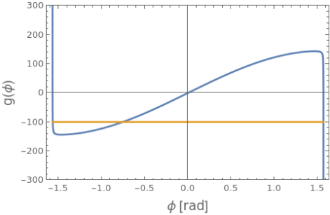
Figure 1: An example of the function $g(\phi)$ from Eq. 10, where $H=145.9$, $G=0.1645$. The orange horizontal line is the value of $W$.

After solving the equation and determining $\phi_{0}$ (using Newton’s method, for instance) and verifying the derivative $g^{\prime}(\phi_{0})$ is positive, we obtain $K=H\sin\phi_{0}$. Using this value, we find $\cos(x)=m/(y\gamma-K)$, and the momentum in the center-of-mass frame is given by $k=m\tan(x)$. The excitation energy $E_{x}$ can then be calculated using Eq. 6 with the mass of the heavy recoil B ($M$):

$$E_{x}=\sqrt{M^{2}+E_{cm}^{2}-2E_{cm}\sqrt{M^{2}+k^{2}}}-M.$$ (11)

The center-of-mass scattering angle, $\theta_{cm}$, can be deduced using Eq. 7.

4 Demonstration & Discussion

A program has been developed to implement this method for HELIOS [3]. The calibration parameters $(a,b)$ are randomly initialized within a specified range, typically $1/a\in(220,320)$ and $b\in(-1,1)$. To demonstrate the method, we applied it to the ²⁵Mg($d$,$p$) reaction at 6 MeV/u under a magnetic field of 2.85 T (Fig. 2).

The threshold $\tau$ was set to 0.1 MeV, approximately matching the energy resolution. The calibration process for the entire detector array required only a few minutes to complete. Following the calibration, the excitation energy and center-of-mass angle were reconstructed and are presented in Fig. 3.

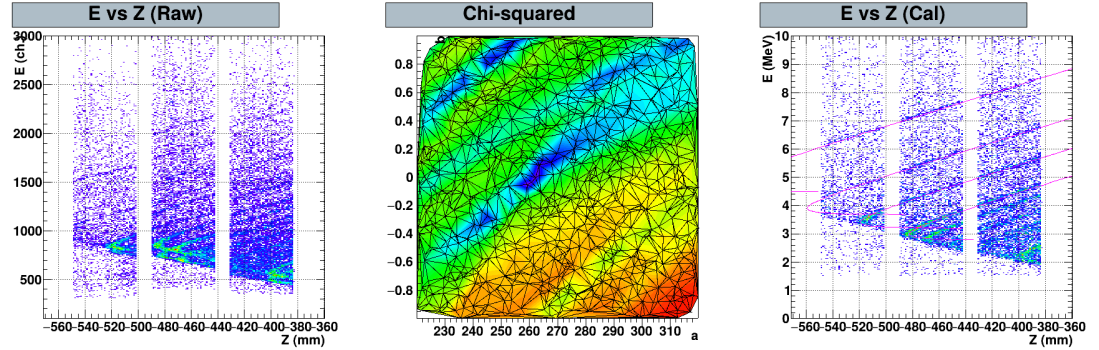
Figure 2: (Left) The $e$-$Z$ plot showing the experimental energy (in channel) versus z-position (in mm) before calibration. (Middle) The parameter space and corresponding $\chi^{2}$ values for a single detector. One thousand random parameter pairs (trials) were generated, and $\chi^{2}$ and $N$ were computed. The lowest $\chi^{2}$ values are depicted in deep blue, while higher values are shown in red. (Right) The calibrated $E$-$Z$ plot. Red curves represent the theoretical kinematic trajectories of ²⁶Mg states used for calibration.

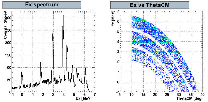
Figure 3: (Left) The excited energy spectrum of ²⁶Mg. (Right) The $E_{x}-\theta_{cm}$ plot. A $\theta_{cm}>10^{\circ}$ cut was applied.

In this demonstration, only the lowest four excited states were used for calibration. The method correctly matched the experimental data, resulting in accurate calibration of higher excited states.

In the raw energy plot (left panel of Fig.2), four detectors are positioned at the same $z$-position. After kinematic calibration, all detectors align well with the theoretical values (right panel of Fig.2).

No background gating was applied during the calibration, yet the results were satisfactory. Applying appropriate gates to clean the data would speed up the calibration process. In the $\chi^{2}$ plot (middle panel of Fig. 2), several local minima are observed. If the number of trials is insufficient, the global minimum may not be identified. The current random parameter sampling could be optimized with a more adaptive search algorithm.

The method may fail if the level density is high, potentially leading to incorrect parameters corresponding to a global minimum that matches a different set of levels. This can occur due to a larger number of data points at higher energies, which increases the count of data points, $N$, and may result in a smaller $\chi^{2}$.

The method remains effective even with just two known states, provided no other pair of states has a similar energy separation and the level density is not too high. This is because the slope of the $E$-$Z$ curves must match the kinematic curves. Additionally, the range of the scaling parameter, $a$, helps exclude spurious minima. If another pair of states has a similar energy separation, the method may incorrectly fit to those states, leading to an incorrect calibration. In general, using more known states improves the reliability of the fit. If high-energy states are unknown, it is advisable to use a gate to select only the known states for calibration.

Compared to alpha calibration, kinematic calibration generally provides better results due to the limited energy range of alpha sources. However, even with alpha calibration alone, the subsequent reconstruction of $E_{x}$ and $\theta_{cm}$ remains acceptable.

For this method to function properly, the $z$-position of the detector array is assumed to be well known. However, if the $z$-position is not accurately determined, the characteristic bending of the $E$-$Z$ relationship at small center-of-mass angles can be used to estimate the $z$-position before performing the kinematic energy calibration.

At very small $\theta_{cm}$, the transformation $(E,Z)\rightarrow(E_{x},\theta_{cm})$ is not unique (or bijective), which can render the experimental data unusable. However, when the level spacing is sufficiently large such that only one state exhibits a distinct bending in its $E$-$Z$ curve, and this curve does not overlap with other states, Eq. 5 can be used to deduce $\theta_{cm}$ for a given $E_{x}$.

5 Summary

A novel method is presented for analyzing data from solenoidal spectrometers used in nuclear reaction studies. These spectrometers measure the energy ($e$) and position ($Z$) of light recoil charged particles, which are related to the excitation energy ($E_{x}$) and center-of-mass scattering angle ($\theta_{cm}$) of the heavy recoil nucleus. Traditional analysis methods, which rely on projecting excitation lines, face challenges at forward angles due to detector geometry effects. Our new approach addresses these limitations by first calibrating the experimental $e$-$Z$ data (in channel - mm) to obtain $E$-$Z$ values using known excited states and a minimum chi-squared fitting procedure with a distance threshold to reject noise. Then, through a series of transformations based on relativistic kinematics and cyclotron motion in the spectrometer’s magnetic field, we derive an analytical relationship that enables a direct inverse transformation from the calibrated $E$-$Z$ data to $E_{x}$ and $\theta_{cm}$. We also propose a method for extracting very small $\theta_{cm}$ values when the state is sufficiently separated from others. This method circumvents the non-linearity of the $E$-$Z$ relationship and ensures consistent treatment of all detectors. The efficacy of this method is demonstrated by applying it to the ²⁵Mg($d$,$p$) reaction. This automated method provides a more robust, speedy, and accurate way to extract excitation energy spectra and angular distributions from solenoidal spectrometers.

6 Acknowledgement

This research utilized resources from Florida State University’s John D. Fox Laboratory, supported by the National Science Foundation under Grant No. PHY-2012522, and Argonne National Laboratory’s ATLAS facility, a Department of Energy Office of Science User Facility supported by the U.S. Department of Energy, Office of Science, Office of Nuclear Physics, under Contract No. DE-AC02-06CH11357.

References

- [1] A.H. Wuosmaa et al., Nuclear Instruments and Method A 580, 1290-1300 (2007)
- [2] T.L. Tang, Kenematics of HELIOS.pdf
- [3] J.C. Lightall et al., Nuclear Instruments and Method A 622, 97-106 (2010)