Inside Out: Externalizing Assumptions in Data Analysis as Validation Checks

Abstract

In data analysis, unexpected results often prompt researchers to revisit their procedures to identify potential issues. While some researchers may struggle to identify the root causes, experienced researchers can often quickly diagnose problems by checking a few key assumptions. These checked assumptions, or expectations, are typically informal, difficult to trace, and rarely discussed in publications. In this paper, we introduce the term analysis validation checks to formalize and externalize these informal assumptions. We then introduce a procedure to identify a subset of checks that best predict the occurrence of unexpected outcomes, based on simulations of the original data. The checks are evaluated in terms of accuracy, determined by binary classification metrics, and independence, which measures the shared information among checks. We demonstrate this approach with a toy example using step count data and a generalized linear model example examining the effect of particulate matter air pollution on daily mortality.

¹ Department of Statistics and Data Sciences, University of Texas at Austin, Texas, United States

1 Introduction

In data analysis, analysts often rely on their prior knowledge or domain expertise to form expectations and assess whether results align with them. When results deviate from these expectations, experienced analysts check assumptions made about the data and during the analysis, but often do so without discussing the underlying reasoning in the publications. While publication of analysis code and data is now a common a requirement for the sake of reproducibility [Peng, 2011], the published code alone is often insufficient for understanding the thought process behind an analysis. Code corresponding to published analyses often reflect the final decisions made about analysis and do not reveal the decisions or assumptions made about the data during the analysis. Thus, a reader looking at published code can often be left with many questions about why certain choices were made.

We might gain insight into analysts’ thought processes by speaking with them directly or watching them work via screencast videos they produce, such as, TidyTuesday screencast videos or think-aloud type studies [e.g. Gu et al., 2024]. However, direct observation of analysis is not scalable and may not always be feasible; creating educational screencast videos requires significant effort from the analysts. Ideally, there could be a way to explicitly communciate these throught processes in the data analysis to others. Even better, if these expectations were machine-readable, we could analyze them and learn from the analysis itself. For example, we could answer questions about whether the checks also apply to other researchers analyzing new data in the same context, whether they reflect common practices in the field, or whether they are specific to the data or analysis at hand. Externalizing these thought processes is a practice that has potential to improve the trustworthiness of the analyses [Yu and Barter, 2024] in general and the trustworthiness of subsequent products, such as machine learning models, that may be built on such analyses. Developing an approach to reveal some of this process without requiring a reader to essentially reconstruct the analysis process from the raw data would provide an improved basis for trusting an analysis result [Peng and Hicks, 2021].

In this paper, we conceptualize these inexplicit expectations as analysis validation checks, which allows us to examine the assumptions made about the data during an analysis. We then introduce a procedure to identify the subset of checks that best predict the occurrence of unexpected outcomes. The procedure, based on simulations of the original data, compares the accuracy and independence of different combinations of analysis validation checks. Accuracy is determined using binary classification metrics (precision and recall) from a logic regression model [Ruczinski et al., 2003], while independence is measures the shared information among checks. The proposed workflow offers a numerical guarantee that the analysis will produce the expected results, assuming the assumptions about the data generating mechanism hold.

The rest of the paper is organized as follows: Section 2 reviews the concepts of diagnosing unexpected outcomes and general data quality checks. Section 3 introduces the concept of analysis validation checks, illustrated with a toy example based on step count data. Section 4 describes the procedure that selects the best subset of checks for understanding the occurrence of unexpected outcomes. Section 5 applies this procedure to a larger example that estimates the effect of particulate matter air pollution on daily mortality. Section 6 summarises the paper and discusses a few key considerations.

2 Related Work

2.1 Diagnosing unexpected outcomes in data analysis

The concept of framing data analysis as a sense-making process was originally presented by Grolemund and Wickham [2014] based on seminal work by Wild and Pfannkuch [1999]. Key to any sense-making process is a model for the world (i.e. expectations for what we might observe) and observed data with which we can compare our expectations. If there is a significant deviation between what we observe and our expectations, then a data analysis must determine what is causing that deviation. A naive approach would be to update our model for the world to match the data, under the assumption that the initial expectation was incorrect. However, experienced analysts know that the reality can be more nuanced than that, with errors occurring in data collection or data processing that can have an impact on final results.

The skill of diagnosing unexpected data analysis results is not one that has received significant attention in the statistics literature. While the concept of diagnosis is often embedded in model checking or data visualization techniques, systematic approaches to identifying the root cause of a general unexpected analysis result are typically not presented [Peng and Parker, 2022]. Furthermore, if interesting information is discovered through model checking or data visualization, there is no formal way to document such discoveries for the next analyst to consider. Peng et al. [2021] proposed a series of exercises for training students in data analysis to diagnose different kinds of analysis problems such as coding errors or outliers. They provide a systematic approach involving working backwards from the analysis result to identify potential causes. There are parallels here to the concept of debugging and testing in software engineering [Donoghue et al., 2021]. For example, Li et al. [2019] found that experienced engineers were generally able to identify problems in code faster than novices, and that the ability to debug code required knowledge that cut across different domains.

If it is true that the speed with which data analysts can identify problems with an analysis is related to their experience working with a given type of data, then there is perhaps room to improve the analytic process by externalizing the aspects that an analyst learns through experience. That way, inexperienced analysts could examine the thought process of an experienced analyst and learn to identify factors that can cause unexpected results to occur.

2.2 Data analysis checks

The concept of data quality has been studied in the literature, with earlier work focusing on defining frameworks – such as dimensions, attributes, and measures – to improve data quality in database and information systems [Wang and Strong, 1996, Batini et al., 2009, Sidi et al., 2012, Woodall et al., 2014, Cai and Zhu, 2015, Cichy and Rass, 2019]. More recently, data validation has been incorporated into frameworks like Google TensorFlow [Polyzotis et al., 2019] to ensure the quality of data for training machine learning models, as well as for supporting business decision-making [Schelter et al., 2018]. With the increasing availability of open data in scientific research, the users of the data are often not the original data collector and may not be aware of all the details or nuances of the data. This encourages researchers to conduct data quality checks before beginning the analytic process, helping to avoid unexpected discoveries later on. In R, packages like skimr [Waring et al., 2022] and dataMaid [Petersen and Ekstrøm, 2019] provide basic data screening and data quality reports, while packages such as assertr [Fischetti, 2023], validate [van der Loo and de Jonge, 2021], and pointblank [Iannone et al., 2024] focuse on providing infustructures that allow users to define customized data quality checks.

The literature on data quality typically focuses on the intrinsic or inherent quality of the data themselves, rather than the data’s relationship to any specific data analysis. So for example, if a column in a data table is expecting numerical data, but we observe a character value in one of the entries, then that occurrence would trigger some sort of data quality check. This type of quality check can be triggered without any knowledge of what the data will ultimately be used for. However, for a given analysis, we may require specific aspects of the data to be true because they affect the result being computed. Conversely, certain types of poor quality data may have little impact on the ultimate result of an analysis (e.g. data that are missing completely at random). Defining data quality in terms of what may affect a specific analysis outcome or result has the potential to open new avenues for defining data checks and for building algorithms for optimizing the collection of checks defined for a specific analysis.

3 Analysis validation checks

Analysis validation checks are assumptions made by the analysts during the analysis, framed as explicit checks that return a binary TRUE or FALSE value based on the data. Inspired by the concept of data validation checks [van der Loo and de Jonge, 2021], which are designed to ensure that datasets meet expected quality before the analysis begins, analysis validation checks reverse the approach: they validate the assumptions about the data necessary for the analysis to produce the expected results, as defined by the analyst. The focus on expected results allows analysis validation checks to encompass a wide range of checks, such as data quality, variable distributions and outliers, bivariate and multivariate relationships, and contextual information relevant to the analysis.

Our proposed analysis validation checks provide insights into an analyst’s thought process and offer the following benefits:

1. Serve as clear checkpoints to support the replication or application of methods to (new) data by programmatically communicating the requirements or assumptions made of the data;

2. Align assumptions among researchers from different domain backgrounds who may have different expectations about the data;

3. Improve analysis transparency, reproducibility, and trustworthiness by externalizing a key part of the analysis process; and

4. Quantify the effectiveness of analysis checks for predicting the expected outcome (see Section 4);

In addition to the above benefits, the development and publication of analysis checks have the potential to help students, inexperienced analysts, and junior researchers develop the skills needed to diagnose unexpected analysis results for a given type of data because the assumptions made about the data are made transparent. The analysis checks can serve as a basis for new analysts to have conversations about the data they are analyzing and to develop a better understanding of the potential data generation process.

3.1 A Toy Example

Consider a 30-day step count experiment in a public health setting. Subjects are instructed to walk at least 8,000 steps each day, with an expected average of 9,000 steps, tracked by a step counter app. With data of this nature, we may expect there to be occasional “low” days due to factors such as unfavorable weather conditions limiting outdoor activities. We may also expect “high” days recorded after an outdoor activities or intense workout. Given the requirements of the study, we form our expectation as follows:

Expectation: The average step count of a given subject is between $[8,500,9,500]$

To diagnose potential reasons why this expectation might fail, we can establish a few analysis validation checks in anticipation of seeing the data. For example, we can check the quantile of the step count, if more than a third of the days fall below 8,000, or more than a third exceed 10,000 steps, this could indicate an excess of low-count or high-count days. Similarly, we may may expect the standard deviation of the step count not to be overly large. These considerations yield the following three analysis validation checks that fail when:

• Check 1: the 60% quantile of the observed step counts is greater than 10,000

• Check 2: the 40% quantile of the observed step counts is less than 8,000, and

• Check 3: the standard deviation of the observed step counts exceeds 2,500.

The cutoff values for these checks would presumably be chosen based on prior experience with these kinds of data, but could also be optimized using the method presented in the next section.

To simulate this data, three normal distributions are used for the daily step counts: $\mathcal{N}(6,000,200)$ for low days, $\mathcal{N}(12,000,200)$ for high days, and $\mathcal{N}(9,000,300)$ for typical days. The number of low and high days can be simulated from a Poisson distribution with $\lambda=8$. Figure 1 displays average step count across 300 simulated 30-day periods.

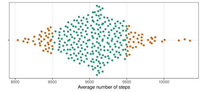
Figure 1: Beeswarm plot of average step counts across 300 simulated 30-day periods. Each point represents the average step count from one simulation. Similar to a boxplot or violin plot, the beeswarm plot also displays the distribution of each individual data point. The orange points indicate instances where the average step count fails outside the [8,500, 9,500] interval, representing an unexpected outcome in this scenario.

4 Method

While not all analysis validation checks are equally important, some may be more useful at diagnosing unexpected outcomes than others. This section introduces a procedure to identify a subset of analysis validation checks that best predict the occurence of unexpected outcomes.

The approach uses simulated datasets that have the same structure and characteristics of the observed data to be analyzed in the future. For each simulated dataset, analysis validation checks are applied to record their TRUE or FALSE values. The outcome of the analysis is also computed to determine whether it is unexpected (1) or expected (0). By generating many datasets, each time applying the analysis validation checks and computing the outcome, we can relate the patterns in the checks to the likely that the outcome will be unexpected. Figure 2 provides an overview of the process.

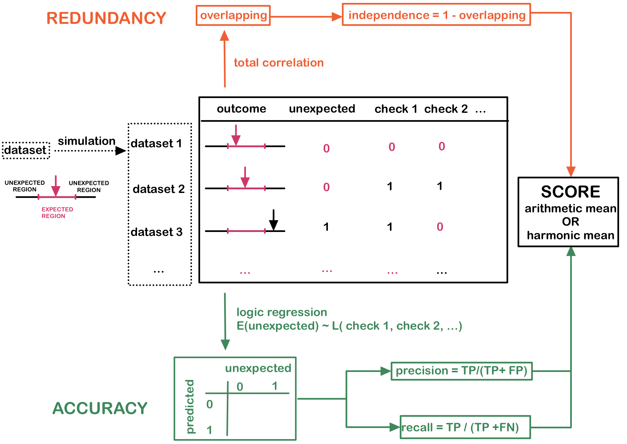
Figure 2: Overview of the procedure to quantify the effectiveness of analysis validation checks. The procedure involves simulating replicates of the data, applying the anlysis, and running the analysis validation checks on each replicate to determine whether the outcome meets the expectation (the unexpected column) and whether each check passes (check 1, check 2, …). The simulation results are then passed to two branches: the accuracy branch calculates the precision and recall of the checks from a logic regression prediction, while the redundancy branch to calculate the mutual information and independence of the checks. These three metrics are combined to produce a single metric that quantifies the effectiveness of the checks in diagnosing unexpected outcomes in the analysis.

4.1 Accuracy

From the simulated data, the accuracy branch in Figure 2 refers to the set of checks’ ability to detect unexpected outcomes accurately. To relate multiple checks to the outcome, a logic regression model [Ruczinski et al., 2003] is used. Originally developed for SNP microarray data, logic regression constructs Boolean combinations of binary variables, $\mathcal{L}(X_{1},X_{2},\cdots,X_{n})$, to predict classification or regression outcomes. The logical operations allowed to construct $\mathcal{L(\cdot)}$ includes AND ($\land$), OR ($\lor$), and NOT ($\neg$) and an example of the Boolean combination of $\mathcal{L(\cdot)}$ is $X_{1}\text{ AND }(X_{2}\text{ OR }X_{3})$. In our binary-binary classification problem, the logic regression model can be written as follows:

$$E(Y)=\mathcal{L}(X_{1},X_{2},\cdots,X_{n})$$

where the outcome, $Y$, indicates whether the outcome is unexpected (1) or expected (0), and the analysis validation checks, $X_{1},X_{2},\cdots,X_{n}$, are labeled as 1 if they fail and 0 if they pass.

This objective function is optimized using simulated annealing algorithm to minimize the misclassification error and the following 6 moves are permitted during the optimization to grow or purne the tree (as detailed in Figure 2 of Ruczinski et al. [2003]): 1) replacing a leaf node, 2) replacing an operator, 3) growing a branch, 4) pruning a branch, 5) splitting a leaf node, and 6) deleting a leaf node. Predictions from the logic regression model is then used, along with the observed outcome, to calculate the precision and recall of the optimized Boolean combination of checks. Compared to other tree-based methods for binary-binary prediction, the Boolean combinations from the logic regression model produce a tree structure that can be directly interpreted as the possible combination of checks leading to an unexpected outcome, without the need to invert the tree as required in classic tree-based recursive partitioning methods.

4.2 Independence

While checks may score high on predictive accuracy, they may be correlated and less useful to provide actions to act on the analysis. This could happen if a set of checks are all tangentially related to the cause of the unexpected results, but none addresses the root cause. The independence score in Figure 2 is defined as 1 - total correlation per observation.

Total correlation is a generalization of mutual information that measures the amount of shared information across multiple variables multiple variables based on Kullback-Leibler distance:

$$C(X_{1},X_{2},\cdots,X_{n})=\sum_{x_{1}}\sum_{x_{2}}\cdots\sum_{x_{n}}p(x_{1},x_{2},\cdots,x_{n})\log\frac{p(x_{1},x_{2},\cdots,x_{n})}{p(x_{1})p(x_{2})\cdots p(x_{n})}$$

A high total correlation value indicates overlapping of information among the analysis validation checks, while a low value suggests that the checks are independent and provides unique information to diagnose the unexpected outcome. To standardize this measure, the total correlation per observation is used in calculating the independence score.

The three metrics (precision, recall, and independence) can be combiend into a single metric using the arithmetic mean, harmonic mean, or quadratic mean. The differences among these means are minimal when the three metrics are similar. However, as the differences among the metrics increases, the harmonic mean tends to produce the smallest overall score, as it penalizes low values, while the quadratic mean tends to produce the largest score by rewarding higher values more. For simple interpretation of the score, the arithmetic mean is preferred, while in applications where the difference between precision, recall, and independence need to be penalized or rewarded more, the harmonic and quadratic mean should be considered.

4.3 Toy Example Revisited

Returning to the step count example introduced in Section 3.1, the logic regression model is fitted to the three validation checks described previously to predict the outcome, whether the average number of step falls within the [8,500, 9,500] interval. Figure 3 shows the best-fitting logic regression model as

(quantile(step, 0.6) > 10,000 OR quantile(step, 0.4) < 8,000) AND (NOT sd(step) > 2,500)

We would predict an unexpected outcome in the analysis if the standard deviation of the step count is not too large (2,500) and either the 60% quantile of the step count exceeds 10,000 or the 40% quantile of the step count falls below 8,000.

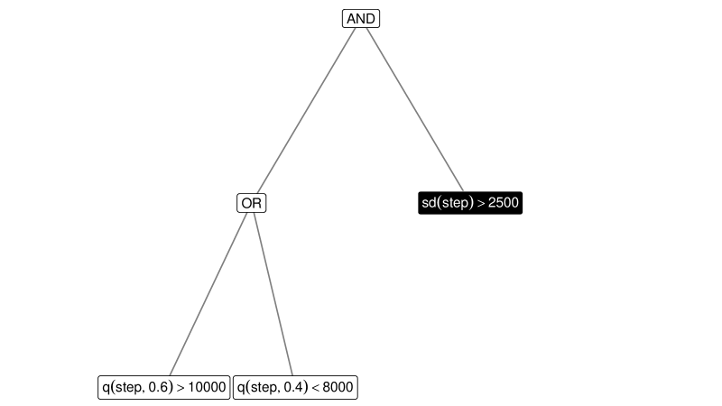
Figure 3: Logic regression model fitted to the three checks. The model suggests the rule (quantile(step, 0.6) > 10,000 OR quantile(step, 0.4) < 8,000) AND (NOT sd(step) > 2,500). The NOT operator applied to sd(step) > 2,500 is colored with a black background to distinguish it from other checks.

Table 1 presents the calculated precision, recall, and independence for the three individual checks and the check rule found by the logic regression. The harmonic and arithmetic means are included to combine the three measures. The results show that the three checks produced by the logic regression can accurately predict 86.1% cases of all predicted unexpected results in the simulation data. Furthermore, 43.1% of all actual unexpected results were in fact observed to be unexpected.

Table 1: Precision, recall, and independence calculated for each individual check and the logic regression check rule. The harmonic and arithmetic means of the three metrics are included to evaluate the quality of the checks in diagnosing unexpected step counts (more than five days with fewer than 8,000 steps).

Checks	Precision	Recall	Independence	Harmonic	Arithmetic
Check 1: q(step, 0.6) > 10000	0.319	0.575	1.000	0.511	0.631
Check 2: q(step, 0.4) < 8000	0.264	0.613	1.000	0.467	0.626
Check 3: sd(step) > 2500	0.153	0.289	1.000	0.273	0.481
Logic regression: (check 1 OR check 2) AND (not check 3)	0.861	0.431	0.998	0.669	0.763
Regression tree	0.542	0.780	1.000	0.727	0.774

For comparison, the regression tree produces a similar prediction to the logic regression, however, we argue that the logic regression tree shown in Figure 3 is more interpretable for our purposes because it provides a direct representation of which combinations of analysis checks lead to unexpected outcomes. The logic regression tree is also directly comparable to other diagnostic techniques, which we discuss further in Section 6.

5 Application

In the study of the health effects of outdoor air pollution, one area of interest is the association between short-term, day-to-day changes in particulate matter air pollution and daily mortality counts. Substantial work has been done to study this question and to date, there appears to be strong evidence of an association between particulate matter less than 10 $\mu$g/m³ in aerodynamic diameter (PM10) and daily mortality from all non-accidental causes [Samet et al., 2000]. For our second example, we use the problem of studying PM10 and mortality along with data from the National Morbidity, Mortality, and Air Pollution Study (NMMAPS) to demonstrate how our analysis validation checks described in Section 4 can be applied. In addition to providing a more substantial problem for our methods, this example also demonstrates how the procedure presented in Section 4 can be used to select cutoff values in the analysis checks to diagnose an unexpected PM10 coefficient from the generalized linear model. The dataset that we use to develop our simulations and analysis checks is from New York City, and contains daily PM10, all-cause (non-accidental) mortality, and average temperature values from 1992–2000. We then will apply the analysis checks to similar data from 39 other cities from the NMMAPS study.

The typical approach to studying the association between PM10 and mortality is to apply a generalized linear model with a Poisson link to relate daily mortality counts to daily measures of PM10. Based on previous work and the range of effect sizes published in the literature, an analyst might expect the coefficient for PM10 in this GLM to lie between $[0,0.005]$, after adjusting for daily temperature [Samet et al., 2000, Welty and Zeger, 2005]. Note that the relatively simple modeling approach being used here is primarily for demonstration; typically far more sophisticated semi-parametric approaches are used in the literature [Peng et al., 2006].

Multiple factors can affect the estimated PM10 coefficient, such as the strength of the correlation between mortality and PM10, or between mortality and temperature. Outliers in the variables can also leverage the coefficient. While these are possible factors that could affect the analysis result, it is not clear what the cutoff values for these checks should be to determine a failure. Here we consider a list of checks in Table LABEL:tbl-checks with varied cutoff values:

Table 2: A list of checks considered for the generalized linear model of mortality on PM10 and temperature. The checks are based on the sample size, correlation between mortality and PM10, correlation between mortality and temperature, and univariate outlier detection. Multiple cutoff values are specified for each check to determine a failure.

The check fails (encoded as 1) if …
Mortality-PM10 correlation less than $-0.05$
Mortality-PM10 correlation less than $-0.03$
Mortality-PM10 correlation greater than $0.03$
Mortality-PM10 correlation greater than $0.05$
Mortality-temperature correlation greater than $-0.3$
Mortality-temperature correlation greater than $-0.35$
Mortality-temperature correlation greater than $-0.4$
Mortality-temperature correlation greater than $-0.45$
Outlier(s) are presented in the variable PM10
Outlier(s) are presented in the variable mortality

5.1 Data Simulation

To generate replicates of the dataset, we first generate the correlation matrix of the three variables (PM10, mortality, and temperature) in a grid and then use a Gaussian copula to generate a multivariate normal distribution based on the specified correlation matrix and sample size. The multivariate normal distribution is transformed using the normal CDF before the inverse CDF of the assumed distributions of the three variables is applied. To determine the appropriate distribution of each variable, various distributions are fitted and compared. This includes poisson and negative binomial for mortality; gamma, log-normal, exponential, weibull, and normal for PM10 and temperature; and beta for PM10 after rescaling the data to $[0,1]$.

To ensure a reasonable likeness to data that might be used in such an analysis, we use characteristics of the observed New York City dataset to refine our simulations. AIC is used to determine the best distribution fit for each variable with the QQ-plot presented in Figure 4 to evaluate the fit. AIC suggests a negative binomial distribution for mortality, a beta distribution for PM10 (multiple by 100 to recover the original scale), and a Weibull distribution for temperature. To include the potential effect of outliers, we add a single outlier to the data for both the mortality and PM10 variables.

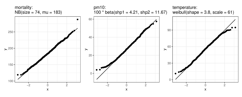
Figure 4: QQ-plot of the distribution fit for mortality, PM10, and temperature based on the fitted distribution from the original data. The fitted distribution is compared to the observed data to assess the distribution fit.

A logic regression is fitted using all variations of the checks in Table LABEL:tbl-checks to predict whether the PM10 coefficient is unexpected. Given the imbalance of outcome (expected vs. unexpected), inverse weights proportional to the number of observations in each outcome are applied during the logic regression fit. Figure 5 shows the optimal logic regression tree from the fitted model. Precision, recall, and independence score, along with their harmonic and arithmetic mean are presented in Table 3.

Figure 5: Logic regression model fitted to the fourteen checks and the outcome expectation (unexpected) as the response variable. The model suggests the relationship: (mortality-PM10 correlation < -0.03) AND (mortality-temperature correlation > -0.3 OR (there exist mortality outlier AND there exist PM10 outlier)) to predict the unexpected PM10 coefficient.

Table 3: Precision, recall, and independence metrics derived from the logic regression model and each individual check, along with harmonic and arithmetic means.

Checks	Precision	Recall	Independence	Harmonic	Arithmetic
Check 1: cor(m, PM10) < -0.03	0.551	0.894	1	0.763	0.815
Check 2: cor(m, tmp) > -0.35	0.281	0.556	1	0.472	0.612
Check 3: mortality outlier	0.302	0.775	1	0.536	0.692
Check 4: PM10 outlier	0.305	0.766	1	0.537	0.690
Logic regression: (check 1) AND ((check 2) OR (check 3 AND check 4))	0.722	0.876	1	0.851	0.866

As indicated in Figure 5, the logic regression model picks up the following cutoff values for each type of check:

• mortality-PM10 correlation less than $-0.03$

• mortality-temperature correlation greater than $-0.3$

• PM10 data contains outliers detected by the univariate outlier detection

• mortality data contains outliers detected by the univariate outlier detection

The fitted logic regression model is

(cor(mortality, PM10) < -0.03) AND (cor(mortality, tmp) > -0.3 OR (mortality outlier AND PM10 outlier))

This generates a precision of 0.722 and a recall of 0.876 for predicting the unexpected PM10 coefficient. As shown in Figure 5, there is no single analysis check in the tree that predicts an unexpected outcome. rather at least three checks in the tree must be TRUE in order for the model to predict an unexpected outcome. Given the high independence of the checks (Table 3), this suggests that unexpected results are only likely after multiple anomalies are observed in the data.

5.2 Additional Cities

In order to test our development of analysis validation checks based on the New York City data, we incorporate data from 39 additional cities from the original NMMAPS study and apply our checks to those data. These cities (along with New York City) represent approximately the largest 40 metropolitan areas in the United States by population. The complete list of cities used are presented in Table 4. For each city, we had daily data on all-cause mortality, PM10, and average temperature for the years 1992–2000.

Table 4: Results from full analysis of 40 cities from the NMMAPS air pollution and mortality study. In the table, a “T” indicates that a check failed and an “F” indicates that a check passed.

City	PM10 Estimated Coefficient	Outcome Observed Unexpected	Logic Regression Predicted Unexpected	Correlation: Mortality- Temperature	Correlation: Mortality- PM10	Mortality Outlier	PM10 Outlier
Atlanta	-0.0008	T	T	–0.26 (T)	–0.16 (T)	F	F
Austin	-0.0030	T	T	–0.12 (T)	–0.11 (T)	F	T
Baltimore	0.0018	F	F	–0.21 (T)	0.01 (F)	T	T
Boston	0.0019	F	F	–0.16 (T)	0.02 (F)	F	T
Buffalo	0.0028	F	F	–0.23 (T)	–0.02 (F)	F	T
Chicago	0.0011	F	F	–0.38 (F)	–0.02 (F)	T	T
Cincinnati	0.0011	F	T	–0.27 (T)	–0.06 (T)	T	T
Cleveland	0.0010	F	F	–0.30 (F)	–0.02 (F)	T	T
Columbus	0.0004	F	T	–0.20 (T)	–0.07 (T)	F	T
Denver	0.0010	F	F	–0.23 (T)	0.06 (F)	F	T
Detroit	0.0011	F	F	–0.30 (T)	0.04 (F)	F	T
Dallas/Fort Worth	0.0016	F	T	–0.30 (F)	–0.03 (T)	T	T
Honolulu	0.0006	F	F	–0.17 (T)	0.05 (F)	T	T
Houston	0.0007	F	F	–0.22 (T)	–0.03 (F)	F	T
Indianapolis	0.0014	F	F	–0.13 (T)	0.02 (F)	F	T
Kansas City	0.0022	F	F	–0.20 (T)	0.02 (F)	F	T
Los Angeles	0.0011	F	F	–0.47 (F)	–0.01 (F)	T	T
Las Vegas	0.0008	F	F	–0.27 (T)	0.05 (F)	T	T
Memphis	-0.0007	T	T	–0.16 (T)	–0.10 (T)	F	T
Miami	-0.0004	T	F	–0.16 (T)	–0.02 (F)	F	T
Milwaukee	0.0026	F	F	–0.22 (T)	0.09 (F)	F	T
Minneapolis/St. Paul	0.0009	F	F	–0.30 (F)	–0.01 (F)	T	T
New York	0.0022	F	F	–0.46 (F)	–0.01 (F)	T	T
Oakland	0.0008	F	F	–0.28 (T)	0.04 (F)	F	T
Orlando	-0.0008	T	T	–0.21 (T)	–0.05 (T)	F	T
Philadelphia	0.0021	F	F	–0.27 (T)	0.11 (F)	T	T
Phoenix	0.0009	F	F	–0.44 (F)	0.07 (F)	T	T
Pittsburgh	0.0009	F	T	–0.36 (F)	–0.08 (T)	T	T
Riverside	0.0001	F	T	–0.27 (T)	–0.11 (T)	T	T
Sacramento	0.0005	F	F	–0.30 (T)	0.05 (F)	T	T
Salt Lake City	-0.0004	T	T	–0.19 (T)	–0.03 (T)	F	T
San Antonio	-0.0021	T	T	–0.22 (T)	–0.16 (T)	F	T
San Bernardino	0.0006	F	T	–0.28 (T)	–0.09 (T)	T	T
San Diego	0.0011	F	F	–0.33 (F)	0.03 (F)	T	T
San Jose	0.0006	F	F	–0.23 (T)	0.08 (F)	F	T
Seattle	0.0003	F	F	–0.24 (T)	0.06 (F)	F	T
Santa Ana/Anaheim	0.0005	F	T	–0.26 (T)	–0.04 (T)	T	T
St. Petersburg	0.0012	F	F	–0.31 (F)	0.01 (F)	F	T
Tampa	-0.0003	T	T	–0.20 (T)	–0.04 (T)	F	T
Tucson	0.0028	F	F	–0.31 (F)	0.18 (F)	T	T

We applied each of the analysis validation checks and the fitted logic regression model separately to each of the cities’ data to make predictions of whether the outcome will be unexpected or not. We also applied the generalized linear model to the data from each of the cities to estimate the association between PM10 and mortality in each city, adjusted for temperature. The estimates of the association and the results of each of the analysis validation checks for each city are shown in Table 4.

Table 5: Summary of the observed and the predicted unexpected PM10 coefficient results from the 40 NMMAPS cities using the logic regression model.

	Predicted
Observed	FALSE	TRUE
FALSE	25	7
TRUE	1	7

It is clear from Table 4 that some of the estimated PM10 coefficients are outside the expected range of [0, 0.005]. Eight of the 40 cities had negative estimated coefficients and were therefore considered unexpected by our original criterion. (It is perhaps worth noting that none of the unexpected outcomes was in the positive direction.) Table 5 summarizes the prediction accuracy of the logic regression model for the 40 cities. The model correctly predicts the PM10 coefficient status of 32 cities, producing an accuracy rate of 80%. Among the 8 cities with an unexpected outcome, the model correctly identifies 7 (Atlanta, Austin, Memphis, Orlando, Salt Lake City, San Antonio, Tampa), giving a recall of 88% (only Miami was not properly classified by the logic regression model). These cities were flagged due to failures in both the mortality-PM10 correlation and mortality-temperature correlation analysis checks. Out of the 14 cities with positive predictions from the model, 7 cities (Cincinnati, Columbus, Dallas/Fort Worth, Pittsburgh, Riverside, San Bernardino, Santa Ana/Anaheim) were false positives, resulting in a precision of only 50%. This precision value is substantially lower than what was estimated by the simulation procedure (see Table 3) and suggests that the simulation does not adequately capture some features of the data generation process.

6 Discussion

In this paper we have developed an approach to using analysis validation checks to externalize the assumptions about the data and analysis tools made during the data analysis process. These checks can serve as a useful summary of the analyst’s thought process and can describe how characteristics of the data may lead to unexpected outcomes. Using logic regression, we can develop a graphical summary of the analysis validation checks as well as use the logic regression fitting process to choose the optimal set of checks. The logic regression model can also be used to develop summaries of the precision and recall of the collection of analysis validation checks in predicting the likelihood of an unexpected outcome. We demonstrated our method on an example relating daily mortality to outdoor air pollution data. The results from that example could be used to inform future analyses of air pollution and health data, perhaps in other cities or locations.

In Section 5 we used the analysis checks in a diagnostic manner to examine the eight cities whose PM10 coefficients were unexpected. There, we found that seven of the cities had a mortality-PM10 correlation that was more negative than expected while also having a mortality-temperature correlation that was somewhat larger (less negative) than expected. What this result implies for the broader analysis depends on a number of factors, but the interplay between mortality, PM10, and temperature may warrant further investigation [see e.g. Welty and Zeger, 2005]. Note that simply because the PM10 coefficient estimates were unexpected by our criterion, we do not mean to imply that they are “wrong” in any sense. Indeed, negative estimated coefficients have been found in other studies of this nature [Bell et al., 2004]. Rather, in this type of analysis, it may be that the interval for expected results needs to be revised. Further, it may be necessary to incorporate other outputs from the analysis, such as measures of uncertainty.

An interesting connection can be drawn between our logic regression trees and a tool used in systems engineering known as a fault tree. A fault tree is used for conducting a structured risk assessment and has a long history in aviation, aerospace, and nuclear power applications [Vesely et al., 1981]. A fault tree is a graphical tool that describes the possible combinations of causes and effects that lead to an anomaly. At the top of the tree is a description of an anomaly. The subsequent branches of the tree below the top event indicate possible causes of the event immediately above it in the tree. The tree can then be built recursively until we reach a root cause that cannot be further investigated. Each level of the tree is connected together using logic gates such as AND and OR gates. The leaf nodes of the tree indicate the root causes that may lead to an anomaly. While the logic regression tress are not identical to fault trees, they share many properties, such as the tree-based structure and the indicator of root causes at the leaf nodes. Perhaps more critically, both serve as graphical summaries of the assumptions made in a problem and the specific violations of those assumptions that could lead to an unexpected result. While fault trees are often used to discover the root cause of an anomaly after it occurs, an important use case for fault trees is to develop a comprehensive understanding of a system before an anomaly occurs [Michael et al., 2002].

Visualization methods are also valuable tools for assessing data assumptions and can potentially be formalized as analysis validation checks. For instance, plotting a variable’s distribution using a histogram, density plot, or bee swarm plot can reveal outliers or deviations from normality. These visualizations could be re-framed as analysis checks that fail when the data does not conform to the visual expectation. However, translating visualization results into binary checks remains an open challenge, requiring either manual verification or the development of automated methods to interpret visualization outputs. An existing example of visual test is the R package vdiffr [Henry et al., 2023] for graphic software unit testing. The package saves a template plot and compares it to the current plot to determine whether the unit tests passes or fails.

Systematically generating realistic simulated data is a key component of our approach and is deserving of further consideration. In the PM10 example in Section 5, the inverse transform method was used to preserve the correlation structure among mortality, PM10, and temperature. However, the simulation process can become complex when additional restrictions are imposed or when a greater range of scenarios is desired. In such cases, techniques like the acceptance-reject method or permutation may be used to generate the data. The results in Section 5 on the broader NMMAPS dataset suggest that our simulation procedure may have been inadequate in reflecting the range of possible configurations that the data could take. In particular, our split-data approach, using New York City to guide the simulation and then applying the analysis checks to other cities, may not have been ideal. It may be worth exploring some recent work in data thinning [Neufeld et al., 2024] and data fission [Leiner et al., 2023] to create training datasets that are more representative of future data.

Analysis validation checks are closely related to the concept of unit testing in software engineering. While unit tests isolate and test specific lines of the code, analysis validation checks focus on the assumptions underlying the analysis rather than the explicit code itself. Moreover, while software testing is deterministic, with clear rules for determining failure, analysis validation checks are probabilistic. As a result, an analysis may fail several assumption checks yet produce an expected outcome, or pass all checks but yield an unexpected result.

Communicating the process of data analysis is a key element to providing transparency, improving reproducibility, and building trust with a range of audiences. The analysis validation checks described here provide a general way to encode the assumptions that an data analyst makes about the data and statistical tools applied to the data. These assumptions can be studied or challenged, depending on the specific analyst’s perspective, and can serve as a roadmap for diagnosing unexpected results.

7 Acknowledgement

The article is created using Quarto [Allaire et al., 2022] in R [R Core Team, 2023]. The source code for reproducing the work reported in this paper can be found at: https://github.com/huizezhang-sherry/paper-avc.

References

- Allaire et al. [2022] J.J. Allaire, Charles Teague, Carlos Scheidegger, Yihui Xie, and Christophe Dervieux. Quarto, January 2022. URL https://github.com/quarto-dev/quarto-cli.
- Batini et al. [2009] Carlo Batini, Cinzia Cappiello, Chiara Francalanci, and Andrea Maurino. Methodologies for data quality assessment and improvement. ACM computing surveys (CSUR), 41(3):1–52, 2009.
- Bell et al. [2004] Michelle L Bell, Aidan McDermott, Scott L Zeger, Jonathan M Samet, and Francesca Dominici. Ozone and short-term mortality in 95 us urban communities, 1987-2000. Jama, 292(19):2372–2378, 2004.
- Cai and Zhu [2015] Li Cai and Yangyong Zhu. The challenges of data quality and data quality assessment in the big data era. Data science journal, 14:2–2, 2015.
- Cichy and Rass [2019] Corinna Cichy and Stefan Rass. An overview of data quality frameworks. IEEE Access, 7:24634–24648, 2019. 10.1109/ACCESS.2019.2899751.
- Donoghue et al. [2021] Thomas Donoghue, Bradley Voytek, and Shannon E Ellis. Teaching creative and practical data science at scale. Journal of Statistics and Data Science Education, 29(sup1):S27–S39, 2021.
- Fischetti [2023] Tony Fischetti. assertr: Assertive Programming for R Analysis Pipelines, 2023. URL https://CRAN.R-project.org/package=assertr. R package version 3.0.1.
- Grolemund and Wickham [2014] Garrett Grolemund and Hadley Wickham. A Cognitive Interpretation of Data Analysis. International Statistical Review, 82(2):184–204, 08 2014. 10.1111/insr.12028. URL https://onlinelibrary.wiley.com/doi/10.1111/insr.12028.
- Gu et al. [2024] Ken Gu, Madeleine Grunde-McLaughlin, Andrew McNutt, Jeffrey Heer, and Tim Althoff. How do data analysts respond to ai assistance? a wizard-of-oz study. In Proceedings of the CHI Conference on Human Factors in Computing Systems, pages 1–22, 2024.
- Henry et al. [2023] Lionel Henry, Thomas Lin Pedersen, T Jake Luciani, Matthieu Decorde, and Vaudor Lise. vdiffr: Visual Regression Testing and Graphical Diffing, 2023. URL https://CRAN.R-project.org/package=vdiffr. R package version 1.0.7.
- Iannone et al. [2024] Richard Iannone, Mauricio Vargas, and June Choe. pointblank: Data Validation and Organization of Metadata for Local and Remote Tables, 2024. URL https://CRAN.R-project.org/package=pointblank. R package version 0.12.2.
- Leiner et al. [2023] James Leiner, Boyan Duan, Larry Wasserman, and Aaditya Ramdas. Data fission: splitting a single data point. Journal of the American Statistical Association, pages 1–12, 2023.
- Li et al. [2019] Chen Li, Emily Chan, Paul Denny, Andrew Luxton-Reilly, and Ewan Tempero. Towards a framework for teaching debugging. In Proceedings of the Twenty-First Australasian Computing Education Conference, pages 79–86, 2019.
- Michael et al. [2002] Stamatelatos Michael, D Joane, F Joseph, M Joseph, and R Jan. Fault tree handbook with aerospace applications. NASA Office of Safety and Mission Assurance-NASA Headquarters, Washington, pages 2–8, 2002.
- Neufeld et al. [2024] Anna Neufeld, Ameer Dharamshi, Lucy L Gao, and Daniela Witten. Data thinning for convolution-closed distributions. Journal of Machine Learning Research, 25(57):1–35, 2024.
- Peng [2011] Roger D Peng. Reproducible research in computational science. Science, 334(6060):1226–1227, 2011.
- Peng and Hicks [2021] Roger D Peng and Stephanie C Hicks. Reproducible research: a retrospective. Annual review of public health, 42(1):79–93, 2021.
- Peng and Parker [2022] Roger D Peng and Hilary S Parker. Perspective on data science. Annual Review of Statistics and Its Application, 9(1):1–20, 2022.
- Peng et al. [2006] Roger D Peng, Francesca Dominici, and Thomas A Louis. Model choice in time series studies of air pollution and mortality. Journal of the Royal Statistical Society Series A: Statistics in Society, 169(2):179–203, 2006.
- Peng et al. [2021] Roger D. Peng, Athena Chen, Eric Bridgeford, Jeffrey T. Leek, and Stephanie C. Hicks. Diagnosing Data Analytic Problems in the Classroom. Journal of Statistics and Data Science Education, 29(3):267–276, September 2021. 10.1080/26939169.2021.1971586. URL https://doi.org/10.1080/26939169.2021.1971586.
- Petersen and Ekstrøm [2019] Anne Helby Petersen and Claus Thorn Ekstrøm. datamaid: Your assistant for documenting supervised data quality screening in r. Journal of Statistical Software, 90:1–38, 2019.
- Polyzotis et al. [2019] Neoklis Polyzotis, Martin Zinkevich, Sudip Roy, Eric Breck, and Steven Whang. Data validation for machine learning. Proceedings of machine learning and systems, 1:334–347, 2019.
- R Core Team [2023] R Core Team. R: A Language and Environment for Statistical Computing. R Foundation for Statistical Computing, Vienna, Austria, 2023. URL https://www.R-project.org/.
- Ruczinski et al. [2003] Ingo Ruczinski, Charles Kooperberg, and Michael LeBlanc. Logic Regression. Journal of Computational and Graphical Statistics, 12(3):475–511, September 2003. ISSN 1061-8600. 10.1198/1061860032238. URL https://doi.org/10.1198/1061860032238. Publisher: ASA Website.
- Samet et al. [2000] Jonathan M Samet, Francesca Dominici, Frank C Curriero, Ivan Coursac, and Scott L Zeger. Fine particulate air pollution and mortality in 20 us cities, 1987–1994. New England journal of medicine, 343(24):1742–1749, 2000.
- Schelter et al. [2018] Sebastian Schelter, Dustin Lange, Philipp Schmidt, Meltem Celikel, Felix Biessmann, and Andreas Grafberger. Automating large-scale data quality verification. Proceedings of the VLDB Endowment, 11(12):1781–1794, 2018.
- Sidi et al. [2012] Fatimah Sidi, Payam Hassany Shariat Panahy, Lilly Suriani Affendey, Marzanah A. Jabar, Hamidah Ibrahim, and Aida Mustapha. Data quality: A survey of data quality dimensions. In 2012 International Conference on Information Retrieval & Knowledge Management, pages 300–304, 2012. 10.1109/InfRKM.2012.6204995.
- van der Loo and de Jonge [2021] Mark PJ van der Loo and Edwin de Jonge. Data validation infrastructure for r. Journal of Statistical Software, 97:1–33, 2021. 10.18637/jss.v097.i10. URL https://www.jstatsoft.org/article/view/v097i10.
- Vesely et al. [1981] William E Vesely, Francine F Goldberg, Norman H Roberts, and David F Haasl. Fault tree handbook. Technical report, Nuclear Regulatory Commission Washington DC, 1981.
- Wang and Strong [1996] Richard Y Wang and Diane M Strong. Beyond accuracy: What data quality means to data consumers. Journal of management information systems, 12(4):5–33, 1996.
- Waring et al. [2022] Elin Waring, Michael Quinn, Amelia McNamara, Eduardo Arino de la Rubia, Hao Zhu, and Shannon Ellis. skimr: Compact and Flexible Summaries of Data, 2022. URL https://CRAN.R-project.org/package=skimr. R package version 2.1.5.
- Welty and Zeger [2005] Leah J Welty and Scott L Zeger. Are the acute effects of particulate matter on mortality in the national morbidity, mortality, and air pollution study the result of inadequate control for weather and season? a sensitivity analysis using flexible distributed lag models. American journal of epidemiology, 162(1):80–88, 2005.
- Wild and Pfannkuch [1999] Chris J Wild and Maxine Pfannkuch. Statistical thinking in empirical enquiry. International statistical review, 67(3):223–248, 1999.
- Woodall et al. [2014] Philip Woodall, Martin Oberhofer, and Alexander Borek. A classification of data quality assessment and improvement methods. International Journal of Information Quality 16, 3(4):298–321, 2014.
- Yu and Barter [2024] Bin Yu and Rebecca L Barter. Veridical data science: The practice of responsible data analysis and decision making. MIT Press, 2024.