A truncated $\varepsilon$-subdifferential method for global DC optimization

Abstract

We consider the difference of convex (DC) optimization problem subject to box-constraints. Utilizing $\varepsilon$-subdifferentials of DC components of the objective, we develop a new method for finding global solutions to this problem. The method combines a local search approach with a special procedure for escaping non-global solutions by identifying improved initial points for a local search. The method terminates when the solution cannot be improved further. The escaping procedure is designed using subsets of the $\varepsilon$-subdifferentials of DC components. We compute the deviation between these subsets and determine $\varepsilon$-subgradients providing this deviation. Using these specific $\varepsilon$-subgradients, we formulate a subproblem with a convex objective function. The solution to this subproblem serves as a starting point for a local search.

We study the convergence of the conceptual version of the proposed method and discuss its implementation. A large number of academic test problems demonstrate that the method requires reasonable computational effort to find higher quality solutions than other local DC optimization methods. Additionally, we apply the new method to find global solutions to DC optimization problems and compare its performance with two benchmark global optimization solvers.

Keywords: Global optimization, DC optimization, Nonsmooth optimization, $\varepsilon$-subdifferential

MSC classes: 90C26, 90C59, 49J52, 65K05

1 Introduction

Consider the following difference of convex (DC) optimization problem with box-constraints:

$$\begin{cases}\text{minimize}\quad&f({\bm{x}})\\ \text{subject to}&{\bm{x}}\in[{\bm{a}},{\bm{b}}],\end{cases}$$ (1)

where $f({\bm{x}})=f_{1}({\bm{x}})-f_{2}({\bm{x}}),~{\bm{a}},{\bm{b}}\in\mathbb{R}^{n},~{\bm{a}}\leq{\bm{b}}$ and $f_{1},~f_{2}:\mathbb{R}^{n}\to\mathbb{R}$ are convex functions. Note that then $f_{1}$ and $f_{2}$, and thus $f$ are all continuous. The presentation $f_{1}-f_{2}$ of the DC function $f$ is called its DC decomposition whereas $f_{1}$ and $f_{2}$ are called DC components. The problem (1) has various applications, for example, in engineering, business and machine learning [10, 13].

Using the exact penalty function approach we can include box-constraints into the first DC component by writing $f_{1}({\bm{x}})+\gamma\,\max\{0,a_{i}-x_{i},x_{i}-b_{i},~i=1,\ldots,n\}$ which is still convex. Here $\gamma>0$ is the penalty parameter. Therefore, without loss of generality, the problem (1) can be replaced by the following unconstrained DC problem:

$$\begin{cases}\text{minimize}\quad&f({\bm{x}})=f_{1}({\bm{x}})-f_{2}({\bm{x}})\\ \text{subject to}&{\bm{x}}\in\mathbb{R}^{n}.\end{cases}$$ (2)

In addition, we assume that $f^{*}=\inf\left\{f({\bm{x}}):~{\bm{x}}\in\mathbb{R}^{n}\right\}>-\infty$.

The problem (2) has been studied by many researchers (see, e.g., [26, 27, 40, 43] and several methods have been developed to solve this DC problem to global optimality [27, 43]. They include a Branch-and-Bound method containing three basic operations: subdivision of simplices, estimation of lower bounds and computation of upper bounds [27]. Versions of the Branch-and-Bound method differ from each other in the way these operations, especially the first operation, are implemented [27, 30, 43]. The outer approximation method was developed in [28, 29]. The decomposition and parametric right-hand-side [43], and the extended cutting angle [20] are other methods for solving global DC programming problems. A survey of some of these methods can be found in [27, 43].

Various local search methods, aiming to find different type of stationary points critical, Clarke stationary, etc.) of DC problems, have also been developed. These methods include the difference of convex algorithm (DCA) and its variations [2, 3, 4, 5, 6], bundle-type methods [1, 14, 19, 22, 31, 32, 38] as well as augmented and aggregate subgradient methods [7, 12]. A brief survey of most of these methods can be found in [39].

DC optimization problems are nonconvex and may have many local minimizers. General purpose global optimization methods are time consuming and may not be efficient if the DC optimization problem has a relatively large number of variables. Although local search methods are computationally efficient, starting from some initial point, they may end up at the closest stationary point where the value of the objective function can be significantly different from that of the global minimizer.

In many real-world applications, local minimizers with an objective value close to that of the global minimizers may still provide satisfactory solutions to the problem. One such application is the hard partitional clustering problem, where an optimal value of its objective reflects the compactness of clusters. In [9], it is shown that the local minimizers of the problem with the objective value close to that of the global minimizers provide similar compact clusters to those by the global minimizer. This observation stimulates the development of DC optimization methods which are able to find high quality solutions in a reasonable time.

In this paper, we develop a new truncated $\varepsilon$-subdifferential (TESGO) method to globally solve the DC optimization problem (2). The method utilizes the DC representation of the objective function. It is a combination of a local search method and a special procedure to escape from solutions which are not global minimizers. More specifically, a local search method is used to compute a stationary point (in our case a critical point) of the DC optimization problem. Then the new escaping procedure is applied to find a better starting point for the local search if the current solution is not a global one. The escaping procedure is designed using subsets of the $\varepsilon$-subdifferentials of DC components. In this procedure, utilizing $\varepsilon$-subgradients we formulate a subproblem with a convex objective function whose solutions are used as starting points for a local search. The TESGO method terminates when the solution found by a local search method cannot be improved anymore. We study the convergence of the conceptual version of the proposed method and discuss its implementation. Using results of numerical experiments we show that TESGO requires a reasonable computational effort to find higher quality solutions than the other four local methods of DC optimization. In addition, we apply TESGO to find global solutions to DC optimization problems and compare its performance with that of two benchmark global optimization solvers.

To the best of our knowledge, this is the first attempt to design a global optimization method when $\varepsilon$-subdifferentials are used with large values of $\varepsilon$ to fulfill the global DC-optimality condition obtained in [25].

The rest of the paper is structured as follows. Section 2 recalls the main notations and some basic definitions from the nonsmooth analysis. The global descent direction is defined in Section 3, where it is shown that such a direction can be computed using the $\varepsilon$-sudifferentials of DC components. The conceptual method is described in Section 4 and its heuristic version is presented in Section 5. In Section 6, the implementation of this method is discussed. Computational results and comparison of TESGO with other methods are studied in Section 7. Finally, Section 8 concludes the paper.

2 Preliminaries

In what follows, we denote by $\mathbb{R}^{n}$ the $n$-dimensional Euclidean space and the vectors of this space with boldface lowercase letters. Furthermore, $\langle{\bm{y}},{\bm{z}}\rangle=\sum_{i=1}^{n}y_{i}z_{i}$ is the inner product of vectors ${\bm{y}},{\bm{z}}\in\mathbb{R}^{n}$, and $\|\cdot\|$ is the associated Euclidean norm. We denote by $S_{1}=\{{\bm{d}}\in\mathbb{R}^{n}:~\|{\bm{d}}\|=1\}$ the unit sphere and by $B_{\varepsilon}({\bm{x}})$ an open ball with the radius $\varepsilon>0$ centred at ${\bm{x}}\in\mathbb{R}^{n}$. The convex hull of a set is denoted by “$\operatorname{conv}$” and the closure of a set by “$\operatorname{cl}$”.

The function $f:\mathbb{R}^{n}\rightarrow\mathbb{R}$ is called locally Lipschitz continuous on $\mathbb{R}^{n}$ if at any point ${\bm{x}}\in\mathbb{R}^{n}$ there exist a constant $L>0$ and a scalar $\varepsilon>0$ such that

$$|f({\bm{y}})-f({\bm{z}})|\leq L\|{\bm{y}}-{\bm{z}}\|\quad\text{for all}~{\bm{y}},{\bm{z}}\in B_{\varepsilon}({\bm{x}}).$$

A direction ${\bm{d}}\in\mathbb{R}^{n}$ is a local descent direction of $f:\mathbb{R}^{n}\rightarrow\mathbb{R}$ at a point ${\bm{x}}\in\mathbb{R}^{n}$ if there exists $\bar{\alpha}>0$ such that $f({\bm{x}}+\alpha{\bm{d}})<f({\bm{x}})$ for all $\alpha\in(0,\bar{\alpha}]$.

The directional derivative of $f:\mathbb{R}^{n}\rightarrow\mathbb{R}$ at ${\bm{x}}\in\mathbb{R}^{n}$ in the direction ${\bm{d}}\in\mathbb{R}^{n}$ is

$$f^{\prime}({\bm{x}};{\bm{d}})=\lim_{t\downarrow 0}\,\,\frac{f({\bm{x}}+t{\bm{d}})-f({\bm{x}})}{t},$$

if it exists. For a finite valued convex function $f:\mathbb{R}^{n}\rightarrow\mathbb{R}$ the directional derivative exits at any ${\bm{x}}\in\mathbb{R}^{n}$ in every direction ${\bm{d}}\in\mathbb{R}^{n}$ and it satisfies [8, 41]

$$f^{\prime}({\bm{x}};{\bm{d}})=\inf_{t>0}\,\,\frac{f({\bm{x}}+t{\bm{d}})-f({\bm{x}})}{t}.$$

The $\varepsilon$-directional derivative for a convex function $f:\mathbb{R}^{n}\rightarrow\mathbb{R}$ at a point ${\bm{x}}\in\mathbb{R}^{n}$ in the direction ${\bm{d}}\in\mathbb{R}^{n}$ is defined as [8, 17]

$$f_{\varepsilon}^{\prime}({\bm{x}};{\bm{d}})=\inf_{t>0}\,\,\frac{f({\bm{x}}+t{\bm{d}})-f({\bm{x}})+\varepsilon}{t}.$$ (3)

The subdifferential of a convex function $f:\mathbb{R}^{n}\rightarrow\mathbb{R}$ at a point ${\bm{x}}\in\mathbb{R}^{n}$ is [8, 41]

$$\partial f({\bm{x}})=\Big{\{}\bm{\xi}\in\mathbb{R}^{n}:~f({\bm{y}})\geq f({\bm{x}})+\langle\bm{\xi},{\bm{y}}-{\bm{x}}\rangle,~\forall\,{\bm{y}}\in\mathbb{R}^{n}\Big{\}}.$$

Each vector $\bm{\xi}\in\partial f({\bm{x}})$ is called a subgradient of $f$ at ${\bm{x}}$. The subdifferential $\partial f({\bm{x}})$ is a nonempty, convex and compact set such that $\partial f({\bm{x}})\subseteq B_{L}(\bm{0})$, where $L>0$ is the Lipschitz constant of $f$ at ${\bm{x}}$.

For $\varepsilon\geq 0$, the $\varepsilon$-subdifferential of a convex function $f:\mathbb{R}^{n}\rightarrow\mathbb{R}$ at a point ${\bm{x}}\in\mathbb{R}^{n}$ is given with [41]

$$\partial_{\varepsilon}f({\bm{x}})=\Big{\{}\bm{\xi}_{\varepsilon}\in\mathbb{R}^{n}:~f({\bm{y}})\geq f({\bm{x}})+\langle\bm{\xi}_{\varepsilon},{\bm{y}}-{\bm{x}}\rangle-\varepsilon,~\forall\,{\bm{y}}\in\mathbb{R}^{n}\Big{\}}.$$

Each vector $\bm{\xi}_{\varepsilon}\in\partial_{\varepsilon}f({\bm{x}})$ is called an $\varepsilon$-subgradient of $f$ at ${\bm{x}}$. The set $\partial_{\varepsilon}f({\bm{x}})$ is nonempty, convex and compact, and it contains the subgradient information from some neighbourhood of ${\bm{x}}$. This is due to the fact that $\partial f({\bm{y}})\subseteq\partial_{\varepsilon}f({\bm{x}})$ for all ${\bm{y}}\in B_{\frac{\varepsilon}{2L}}({\bm{x}})$, where $L>0$ is the Lipschitz constant of $f$ at ${\bm{x}}$ (see Theorem 2.33 in [8]).

For a locally Lipschitz continuous function $f:\mathbb{R}^{n}\rightarrow\mathbb{R}$, the Clarke subdifferential at a point ${\bm{x}}\in\mathbb{R}^{n}$ is defined as [15]

$$\partial_{C}f({\bm{x}})=\operatorname{conv}\left\{\lim_{i\rightarrow\infty}\nabla f({\bm{x}}_{i})\,:\,{\bm{x}}_{i}\rightarrow{\bm{x}}\text{ and }\nabla f({\bm{x}}_{i})\text{ exists}\right\},$$

and, similarly to the convex case, each $\bm{\xi}\in\partial_{C}f({\bm{x}})$ is called a subgradient. Moreover, $\partial_{C}f({\bm{x}})=\partial f({\bm{x}})$ for a convex function $f$.

The Goldstein $\varepsilon$-subdifferential of a locally Lipschitz continuous function $f:\mathbb{R}^{n}\rightarrow\mathbb{R}$ at a point ${\bm{x}}\in\mathbb{R}^{n}$ for $\varepsilon\geq 0$ is defined by [23]

$$\partial_{\varepsilon}^{G}f({\bm{x}})=\operatorname{cl}\,\operatorname{conv}~\bigcup_{{\bm{y}}\,\in\,{B}_{\varepsilon}({\bm{x}})}\partial f({\bm{y}}).$$

The set $\partial_{\varepsilon}^{G}f({\bm{x}})$ coincides with $\partial_{C}f({\bm{x}})$ with the selection $\varepsilon=0$, and for any $\varepsilon\geq 0$ we have $\partial_{C}f({\bm{x}})\subseteq\partial_{\varepsilon}^{G}f({\bm{x}})$. Thus, the Goldstein $\varepsilon$-subdifferential can be used to approximate the Clarke subdifferential and, in the convex case, the subdifferential. Moreover, for a convex function $f$ we have $\partial_{\varepsilon}^{G}f({\bm{x}})\subseteq\partial_{2L\varepsilon}f({\bm{x}})$, where $L>0$ is its Lipschitz constant at a point ${\bm{x}}\in\mathbb{R}^{n}$ (see Theorem 3.11 in [8]).

Note that the execution of a local search method is stopped when a stationary point ${\bm{x}}^{*}\in\mathbb{R}^{n}$ is reached. For the DC problem (2), the most common option is a critical point fulfilling the condition $\partial f_{1}({\bm{x}}^{*})\cap\partial f_{2}({\bm{x}}^{*})\neq\emptyset$. The set of critical points contains all global and local minimizers as well as Clarke stationary points satisfying the condition $\bm{0}\in\partial_{C}f({\bm{x}})$ at a point ${\bm{x}}\in\mathbb{R}^{n}$. In addition, inf-stationary points fulfilling the condition $\partial f_{2}({\bm{x}})\subseteq\partial f_{1}({\bm{x}})$ at ${\bm{x}}\in\mathbb{R}^{n}$ are included in the set of critical points. Moreover, at a local minimizer ${\bm{x}}^{*}\in\mathbb{R}^{n}$, criticality, Clarke stationarity and inf-stationarity are satisfied. In what follows, we use the term critical point whenever we talk about stationary points.

Quality of solutions.

Since DC optimization problems are nonconvex, they may have many local minimizers including global ones. Some of the local minimizers are closer (in the sense of the objective value) to the global minimizer than others. This raises the question about the accuracy of local minimizers with respect to global minimizers (or the best known local minimizers).

Let $U$ be a set of critical points and $U^{*}$ be a set of global minimizers (or best known local minimizers) of the problem (2). It is clear that $U^{*}\subseteq U$. Set $f^{*}=f({\bm{x}}^{*})$ for ${\bm{x}}^{*}\in U^{*}$ and take any ${\bm{x}}\in U$. Then the accuracy (relative error) of the critical point ${\bm{x}}$ is defined as

$$E({\bm{x}})=\frac{f({\bm{x}})-f^{*}}{|f^{*}|+1}.$$ (4)

It is clear that $E({\bm{x}})\geq 0$. We say that the critical point ${\bm{x}}\in U$ is higher quality than the critical point ${\bm{y}}\in U$ if $E({\bm{x}})<E({\bm{y}})$. For a given $\tau>0$, the critical point ${\bm{x}}\in U$ is called the $\tau$-approximate global minimizer of the problem (2) if $E({\bm{x}})\leq\tau$.

3 Global optimality condition and escaping procedure

Consider the problem (2). The following theorem and corollary on global optimality conditions were established in [25].

Theorem 1

For ${\bm{x}}^{*}\in\mathbb{R}^{n}$ to be a global minimizer of the problem (2) it is necessary and sufficient that

$$\partial_{\varepsilon}f_{2}({\bm{x}}^{*})\subseteq\partial_{\varepsilon}f_{1}({\bm{x}}^{*})\quad\text{for all}~\varepsilon\geq 0.$$ (5)

Corollary 1

Let ${\bm{x}}^{*}\in\mathbb{R}^{n}$ be a global minimizer of the problem (2) and $f^{*}=f({\bm{x}}^{*})$. Let also $\bar{{\bm{x}}}\in\mathbb{R}^{n}$ be a local minimizer of the problem (2) and $\bar{f}=f(\bar{{\bm{x}}})$. Set $\alpha=\bar{f}-f^{*}\geq 0$. Then

$$\partial_{\varepsilon}f_{2}(\bar{{\bm{x}}})\subseteq\partial_{\varepsilon+\alpha}f_{1}(\bar{{\bm{x}}})\quad\text{for all}~\varepsilon\geq 0.$$

From the definition of the $\varepsilon$-approximate global minimizers and Corollary 1 we get the following corollary.

Corollary 2

Let $\bar{\varepsilon}\geq 0$ and $\bar{{\bm{x}}}\in U$ be an $\bar{\varepsilon}$-approximate global minimizer. Then

$$\partial_{\varepsilon}f_{2}(\bar{{\bm{x}}})\subseteq\partial_{\varepsilon+\hat{\varepsilon}}f_{1}(\bar{{\bm{x}}})\quad\text{for all}~\varepsilon\geq 0$$

where $\hat{\varepsilon}=\bar{\varepsilon}(|f^{*}|+1)$.

Theorem 1 implies that if the point $\bar{{\bm{x}}}\in\mathbb{R}^{n}$ is a local minimizer but not a global one, then the condition (5) is not satisfied for some $\varepsilon>0$ and there exists ${\bm{y}}\in\mathbb{R}^{n}$ such that $f({\bm{y}})<f(\bar{{\bm{x}}})$. This leads to the following definition of the global descent direction.

Definition 1

Let $\bar{{\bm{x}}}\in\mathbb{R}^{n}$ be a local minimizer of the problem (2). A direction ${\bm{d}}\in\mathbb{R}^{n},{\bm{d}}\neq\bm{0}$ is called a global descent direction of the function $f$ at the point $\bar{{\bm{x}}}$ if there exist $\bar{\alpha}>0$ and $\delta\in(0,\bar{\alpha})$ such that $f(\bar{{\bm{x}}}+\alpha{\bm{d}})<f(\bar{{\bm{x}}})$ for all $\alpha\in(\bar{\alpha}-\delta,\bar{\alpha}+\delta)$.

Note that the global descent directions are defined at local minimizers. This is due to the fact that at any other point, there always exists local descent directions. However, local descent directions do not exist at local minimizers.

Next, we prove that if at the local minimizer $\bar{{\bm{x}}}\in\mathbb{R}^{n}$ the optimality condition (5) is not satisfied, $\varepsilon$-subdifferentials of DC components can be used to compute global descent directions at this point.

Theorem 2

Let $\bar{{\bm{x}}}\in\mathbb{R}^{n}$ be a local minimizer of the problem (2). If the condition (5) is satisfied at $\bar{{\bm{x}}}\in\mathbb{R}^{n}$, then it is a global minimizer. Otherwise, there exists a global descent direction at this point.

Proof 1

If the condition (5) is satisfied at the local minimizer $\bar{{\bm{x}}}\in\mathbb{R}^{n}$ for any $\varepsilon\geq 0$, then according to Theorem 1 $\bar{{\bm{x}}}$ is a global minimizer.

Now assume that a point $\bar{{\bm{x}}}\in\mathbb{R}^{n}$ is a local minimizer but not a global one. Then there exists $\bar{\varepsilon}>0$ such that

$$\partial_{\bar{\varepsilon}}f_{2}(\bar{{\bm{x}}})\nsubseteq\partial_{\bar{\varepsilon}}f_{1}(\bar{{\bm{x}}}),$$

as a local minimizer is always an inf-stationary point. This means that there exists $\bar{\bm{\xi}}_{2}\in\partial_{\bar{\varepsilon}}f_{2}(\bar{{\bm{x}}})$ such that $\bar{\bm{\xi}}_{2}\notin\partial_{\bar{\varepsilon}}f_{1}(\bar{{\bm{x}}})$. Construct the convex function

$$\hat{f}({\bm{y}})=f_{1}({\bm{y}})-\Big{[}f_{2}(\bar{{\bm{x}}})+\langle\bar{\bm{\xi}}_{2},{\bm{y}}-\bar{{\bm{x}}}\rangle-\bar{\varepsilon}\Big{]},\quad{\bm{y}}\in\mathbb{R}^{n}.$$ (6)

Then we have

$$\hat{f}(\bar{{\bm{x}}})=f_{1}(\bar{{\bm{x}}})-f_{2}(\bar{{\bm{x}}})+\bar{\varepsilon},$$

or

$$f(\bar{{\bm{x}}})=\hat{f}(\bar{{\bm{x}}})-\bar{\varepsilon}.$$ (7)

Note that, the function $\hat{f}$ can be represented as a sum of two convex functions: $f_{1}$ and $h({\bm{y}})=-f_{2}(\bar{{\bm{x}}})-\langle\bar{\bm{\xi}}_{2},{\bm{y}}-\bar{{\bm{x}}}\rangle+\bar{\varepsilon}$. Since ${h}$ is a linear function of ${\bm{y}}$ for any $\varepsilon\geq 0$ we have

$$\partial_{\varepsilon}h({\bm{y}})=\Big{\{}-\bar{\bm{\xi}}_{2}\Big{\}}.$$

Then applying the formula for the $\varepsilon$-subdifferential of the sum of two convex functions [17] and taking into account that for a convex function $f$ we have $\partial_{\varepsilon_{1}}f({\bm{x}})\subseteq\partial_{\varepsilon}f({\bm{x}})$ for all $0\leq\varepsilon_{1}\leq\varepsilon$ (see Theorem 2.32 (ii) in [8]), we obtain

$$\begin{array}[]{lrl}\partial_{\varepsilon}\hat{f}({\bm{y}})&=&\operatorname{conv}\bigcup\limits_{\begin{subarray}{c}\varepsilon_{1}+\varepsilon_{2}=\varepsilon\\ \varepsilon_{1},\varepsilon_{2}\geq 0\end{subarray}}\Big{[}\partial_{\varepsilon_{1}}f_{1}({\bm{y}})+\partial_{\varepsilon_{2}}{h}({\bm{y}})\Big{]}\\ &=&\operatorname{conv}\bigcup\limits_{\varepsilon_{1}\in[0,\varepsilon]}\Big{[}\partial_{\varepsilon_{1}}f_{1}({\bm{y}})-\bar{\bm{\xi}}_{2}\Big{]}\\ &=&\partial_{\varepsilon}f_{1}({\bm{y}})-\bar{\bm{\xi}}_{2}.\end{array}$$

This means that the $\varepsilon$-subdifferential of the function $\hat{f}$ at a point ${\bm{y}}\in\mathbb{R}^{n}$ is

$$\partial_{\varepsilon}\hat{f}({\bm{y}})=\operatorname{conv}\Big{\{}\bm{\xi}\in\mathbb{R}^{n}:~~\bm{\xi}_{1}\in\partial_{\varepsilon}f_{1}({\bm{y}}),\,\,\bm{\xi}=\bm{\xi}_{1}-\bar{\bm{\xi}}_{2}\Big{\}}.$$ (8)

Since $\bar{\bm{\xi}}_{2}\notin\partial_{\bar{\varepsilon}}f_{1}(\bar{{\bm{x}}})$ it follows that $\bm{0}\notin\partial_{\bar{\varepsilon}}\hat{f}(\bar{{\bm{x}}})$.

In addition, from $\bar{\bm{\xi}}_{2}\in\partial_{\bar{\varepsilon}}f_{2}(\bar{{\bm{x}}})$ we get

$$f_{2}({\bm{y}})\geq f_{2}(\bar{{\bm{x}}})+\langle\bar{\bm{\xi}}_{2},{\bm{y}}-\bar{{\bm{x}}}\rangle-\bar{\varepsilon}\quad\text{for all}~{\bm{y}}\in\mathbb{R}^{n},$$

and therefore,

$$f({\bm{y}})=f_{1}({\bm{y}})-f_{2}({\bm{y}})\leq f_{1}({\bm{y}})-\Big{[}f_{2}(\bar{{\bm{x}}})+\langle\bar{\bm{\xi}}_{2},{\bm{y}}-\bar{{\bm{x}}}\rangle-\bar{\varepsilon}\Big{]}=\hat{f}({\bm{y}})\quad\text{for all}~{\bm{y}}\in\mathbb{R}^{n}.$$ (9)

This together with (7) implies that

$$f({\bm{y}})-f(\bar{{\bm{x}}})\leq\hat{f}({\bm{y}})-\hat{f}(\bar{{\bm{x}}})+\bar{\varepsilon}\quad\text{for all }{\bm{y}}\in\mathbb{R}^{n}.$$ (10)

Next, we compute

$$\bar{\bm{\xi}}=\mathop{\mathrm{argmin}}_{\bm{\xi}\in\partial_{\bar{\varepsilon}}\hat{f}(\bar{{\bm{x}}})}~\|\bm{\xi}\|.$$

Since $\bm{0}\notin\partial_{\bar{\varepsilon}}\hat{f}(\bar{{\bm{x}}})$ we have $\|\bar{\bm{\xi}}\|>0$. Applying the necessary and sufficient condition for optimality (Lemma 5.2.6 in [35]) for any $\bm{\xi}\in\partial_{\bar{\varepsilon}}\hat{f}(\bar{{\bm{x}}})$ we obtain

$$\langle\bar{\bm{\xi}},\bm{\xi}-\bar{\bm{\xi}}\rangle\geq 0,$$

which can be rewritten as

$$\langle-\bar{\bm{\xi}},\bm{\xi}\rangle\leq-\|\bar{\bm{\xi}}\|^{2}.$$

The $\varepsilon$-directional derivative of the function $\hat{f}$ at the point $\bar{{\bm{x}}}$ in the direction ${\bm{d}}$ with the selection $\varepsilon=\bar{\varepsilon}$ is (Theorem 2.32 in [8])

$$\hat{f}^{\prime}_{\bar{\varepsilon}}(\bar{{\bm{x}}},{\bm{d}})=\max_{\bm{\xi}\in\partial_{\bar{\varepsilon}}\hat{f}(\bar{{\bm{x}}})}\langle\bm{\xi},{\bm{d}}\rangle.$$

Then for ${\bm{d}}=-\bar{\bm{\xi}}$ we have

$$\hat{f}^{\prime}_{\bar{\varepsilon}}(\bar{{\bm{x}}},{\bm{d}})\leq-\|\bar{\bm{\xi}}\|^{2}.$$ (11)

On the other hand, it follows from (3) that

$$\hat{f}^{\prime}_{\bar{\varepsilon}}(\bar{{\bm{x}}},{\bm{d}})=\inf_{\alpha>0}\frac{\hat{f}(\bar{{\bm{x}}}+\alpha{\bm{d}})-\hat{f}(\bar{{\bm{x}}})+\bar{\varepsilon}}{\alpha}.$$

This together with (11) implies that there exists $\bar{\alpha}>0$ such that

$$\hat{f}(\bar{{\bm{x}}}+\bar{\alpha}{\bm{d}})-\hat{f}(\bar{{\bm{x}}})+\bar{\varepsilon}<-\bar{\alpha}\|\bar{\bm{\xi}}\|^{2}/2.$$ (12)

Then applying (10) for ${\bm{y}}=\bar{{\bm{x}}}+\bar{\alpha}{\bm{d}}$ we obtain

$$f(\bar{{\bm{x}}}+\bar{\alpha}{\bm{d}})-f(\bar{{\bm{x}}})<-\bar{\alpha}\|\bar{\bm{\xi}}\|^{2}/2<0.$$

Since the function $f$ is continuous there exists $\delta\in(0,\bar{\alpha})$ such that

$$f(\bar{{\bm{x}}}+\alpha{\bm{d}})-f(\bar{{\bm{x}}})<-\alpha\|\bar{\bm{\xi}}\|^{2}/4<0$$

for all $\alpha\in(\bar{\alpha}-\delta,\bar{\alpha}+\delta)$. This means that the direction ${\bm{d}}=-\bar{\bm{\xi}}$ is the direction of global descent. $\square$

Theorem 2 shows that if at a local minimizer $\bar{{\bm{x}}}\in\mathbb{R}^{n}$ (not a global one) for some $\bar{\varepsilon}>0$ there exists $\bar{\bm{\xi}}_{2}\in\partial_{\bar{\varepsilon}}f_{2}(\bar{{\bm{x}}})$ such that $\bar{\bm{\xi}}_{2}\notin\partial_{\bar{\varepsilon}}f_{1}(\bar{{\bm{x}}})$, then the $\bar{\varepsilon}$-subgradient $\bar{\bm{\xi}}_{2}$ can be used to find a global descent direction at $\bar{{\bm{x}}}$. In general, there are infinitely many such $\bar{\varepsilon}$-subgradients. For example, we can define $\bar{\bm{\xi}}_{2}$ as follows:

$$\bar{\bm{\xi}}_{2}=\mathop{\mathrm{argmax}}_{\bm{\xi}_{2}\in\partial_{\bar{\varepsilon}}f_{2}(\bar{{\bm{x}}})}\text{ min}\,\Big{\{}\|\bm{\xi}_{1}-\bm{\xi}_{2}\|\,:\,\bm{\xi}_{1}\in\partial_{\bar{\varepsilon}}f_{1}(\bar{{\bm{x}}})\Big{\}}.$$

Theorem 3

Let

• the point $\bar{{\bm{x}}}$ be a local minimizer, but not a global minimizer of the function $f$;

• $\bar{\bm{\xi}}_{2}\in\partial_{\bar{\varepsilon}}f_{2}(\bar{{\bm{x}}})$ and $\bar{\bm{\xi}}_{2}\notin\partial_{\bar{\varepsilon}}f_{1}(\bar{{\bm{x}}})$ for some $\bar{\varepsilon}>0$;

• the function $\hat{f}$ be defined by (6);

• $\bar{\bm{\xi}}_{1}=\mathop{\mathrm{argmin}}\limits_{\bm{\xi}_{1}\in\partial_{\bar{\varepsilon}}f_{1}(\bar{{\bm{x}}})}\big{\|}\bm{\xi}_{1}-\bar{\bm{\xi}}_{2}\big{\|}.$

Then the function $\hat{f}$ is an overestimate of the function $f$, that is $f({\bm{y}})\leq\hat{f}({\bm{y}})$ for all ${\bm{y}}\in\mathbb{R}^{n}$. Furthermore, the point $\bar{{\bm{x}}}$ is not the global minimizer of $\hat{f}$ over $\mathbb{R}^{n}$ and there exists $\bar{\alpha}>0$ such that

$$\hat{f}\Big{(}\bar{{\bm{x}}}-\bar{\alpha}\big{(}\bar{\bm{\xi}}_{1}-\bar{\bm{\xi}}_{2}\big{)}\Big{)}-\hat{f}\big{(}\bar{{\bm{x}}}\big{)}\leq-\bar{\varepsilon}-\frac{\bar{\alpha}}{2}\big{\|}\bar{\bm{\xi}}_{1}-\bar{\bm{\xi}}_{2}\big{\|}^{2},$$ (13)

and

$$f\Big{(}\bar{{\bm{x}}}-\bar{\alpha}\big{(}\bar{\bm{\xi}}_{1}-\bar{\bm{\xi}}_{2}\big{)}\Big{)}-f\big{(}\bar{{\bm{x}}}\big{)}\leq-\frac{\bar{\alpha}}{2}\big{\|}\bar{\bm{\xi}}_{1}-\bar{\bm{\xi}}_{2}\big{\|}^{2}.$$ (14)

Proof 2

The fact that the function $\hat{f}$ is an overestimate of the function $f$ follows from (9). The subdifferential of the function $\hat{f}$ at a point ${\bm{y}}\in\mathbb{R}^{n}$ is $\partial\hat{f}({\bm{y}})=\partial f_{1}({\bm{y}})-\bar{\bm{\xi}}_{2}$ and at the point $\bar{\bm{x}}$ is $\partial\hat{f}(\bar{{\bm{x}}})=\partial f_{1}(\bar{{\bm{x}}})-\bar{\bm{\xi}}_{2}.$ Since $\bar{\bm{\xi}}_{2}\notin\partial_{\bar{\varepsilon}}f_{1}(\bar{{\bm{x}}})$ and $\partial f_{1}(\bar{{\bm{x}}})\subseteq\partial_{\bar{\varepsilon}}f_{1}(\bar{{\bm{x}}})$ it follows that $\bar{\bm{\xi}}_{2}\notin\partial f_{1}(\bar{{\bm{x}}})$. This implies that $\bm{0}\notin\partial\hat{f}(\bar{{\bm{x}}})$. As $\hat{f}$ is convex function we get that $\bar{{\bm{x}}}$ is not a global minimizer of $\hat{f}$. The inequality (13) then follows from (12). According to (9), we have

$$f\left(\bar{{\bm{x}}}-\bar{\alpha}(\bar{\bm{\xi}}_{1}-\bar{\bm{\xi}}_{2})\right)\leq\hat{f}\left(\bar{{\bm{x}}}-\bar{\alpha}(\bar{\bm{\xi}_{1}}-\bar{\bm{\xi}}_{2})\right).$$

Then applying (7), the inequality (14) follows from (13). $\square$

Theorem 3 implies that if a local minimizer $\bar{{\bm{x}}}\in\mathbb{R}^{n}$ is not a global minimizer of the DC function $f$, then we can find $\bar{\varepsilon}>0$ and the $\bar{\varepsilon}$-subgradient $\bar{\bm{\xi}}_{2}\in\partial_{\bar{\varepsilon}}f_{2}({\bm{x}})$ such that $\bar{\bm{\xi}}_{2}\notin\partial_{\bar{\varepsilon}}f_{1}({\bm{x}})$. Then we construct the function $\hat{f}$ using the $\bar{\varepsilon}$-subgradient $\bar{\bm{\xi}}_{2}$ and compute a point where the value of the function $f$ is significantly less than that of at $\bar{{\bm{x}}}$ by solving the problem

$$\mbox{minimize}~~\hat{f}({\bm{x}})~~\mbox{subject~to}~~{\bm{x}}\in\mathbb{R}^{n}.$$ (15)

This means that by solving the problem (15) one can escape from the local minimizers $\bar{{\bm{x}}}$ and find a better starting point for a local search.

Next, using a DC function $f$ of one variable we illustrate graphs of the function $f$ and its corresponding function $\hat{f}$.

Example 1

Consider the DC function $f(x)=f_{1}(x)-f_{2}(x),~x\in\mathbb{R},$ where

$$f_{1}(x)=x^{2}-5x+2,~~~f_{2}(x)=\max\{-3x+8,x+1,5x-12\}.$$

Then

$$f(x)=\min\{x^{2}-2x-6,x^{2}-6x+1,x^{2}-10x+14\}.$$

The point $\bar{x}=1$ is a local minimizer, but not a global one, of the function $f$. It can be shown that $1.1\in\partial_{\bar{\varepsilon}}f_{2}(1)=[-3,13/9]$ but $1.1\notin\partial_{\bar{\varepsilon}}f_{1}(1)=[-7,1]$ for $\bar{\varepsilon}=4$. Then

$$\hat{f}(x)=x^{2}-6.1x+2.1.$$

It is easy to check that $f(1)=\hat{f}(1)-4$. The graphs of the functions $f$ (blue graph) and $\hat{f}$ (dashed red graph) are depicted in Figure 1. We can see that although the function $\hat{f}$ is constructed at the point $x=1$, its minimizer is located in the more deeper basin of the function $f$.

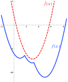
Figure 1: The graph of the function $f$ (blue) with its overestimation $\hat{f}$ (dashed red).

4 Conceptual algorithm

Using results from Theorems 2 and 3, we next introduce Algorithm 1 presenting the conceptual method for globally solving the problem (2).

Algorithm 1 Conceptual algorithm

1: Select any starting point ${\bm{x}}_{0}\in\mathbb{R}^{n}$ and set $k=0$.

2: Apply a local search method starting from the point ${\bm{x}}_{k}$ and find a critical point $\bar{{\bm{x}}}_{k}$.

3: If $\partial_{\varepsilon}f_{2}(\bar{{\bm{x}}}_{k})\subseteq\partial_{\varepsilon}f_{1}(\bar{{\bm{x}}}_{k})$ for any $\varepsilon\geq 0$, then STOP. The point $\bar{{\bm{x}}}_{k}$ is a global minimizer.

4: Find $\bar{\varepsilon}\geq 0$, $\bar{\bm{\xi}}_{1}\in\partial_{\bar{\varepsilon}}f_{1}(\bar{{\bm{x}}}_{k})$ and $\bar{\bm{\xi}}_{2}\in\partial_{\bar{\varepsilon}}f_{2}(\bar{{\bm{x}}}_{k})$ such that

$$\|\bar{\bm{\xi}}_{1}-\bar{\bm{\xi}}_{2}\|^{2}=\max_{\bm{\xi}_{2}\in\partial_{\bar{\varepsilon}}f_{2}(\bar{{\bm{x}}}_{k})}\min_{\bm{\xi}_{1}\in\partial_{\bar{\varepsilon}}f_{1}(\bar{{\bm{x}}}_{k})}\|\bm{\xi}_{1}-\bm{\xi}_{2}\|^{2}>0.$$

5: Construct the function $\hat{f}({\bm{y}})=f_{1}({\bm{y}})-\Big{[}f_{2}(\bar{{\bm{x}}}_{k})+\langle\bar{\bm{\xi}}_{2},{\bm{y}}-\bar{{\bm{x}}}_{k}\rangle-\bar{\varepsilon}\Big{]}$ and solve the problem

$$\mbox{minimize}~~\hat{f}({\bm{y}})~~~\mbox{subject~to}~~{\bm{y}}\in\mathbb{R}^{n}.$$

Let $\bar{{\bm{y}}}$ be a solution to this problem.

6:Set ${\bm{x}}_{k+1}=\bar{{\bm{y}}}$, $k=k+1$ and go to Step 2.

In Algorithm 1, Steps 3$-$5 are, in general, time consuming. In Step 3, we verify that the obtained critical point $\bar{\bm{x}}_{k}\in\mathbb{R}^{n}$ satisfies global optimality. It involves the calculation of $\varepsilon$-subdifferentials of DC components for any $\varepsilon\geq 0$. This step requires the calculation of the whole $\varepsilon$-subdifferential and in general, may not be carried out in a reasonable time. In Step 4, for a given $\bar{\varepsilon}\geq 0$ we compute the deviation of the set $\partial_{\bar{\varepsilon}}f_{2}(\bar{\bm{x}}_{k})$ from the set $\partial_{\bar{\varepsilon}}f_{1}(\bar{\bm{x}}_{k})$. If both sets are polytopes then this problem can be replaced by the finite number of quadratic programming problems which can be solved efficiently applying existing algorithms [21, 33, 37, 44]. Finally, in Step 5 we solve a subproblem to improve the current local minimizer. This problem is a convex optimization problem which can be solved efficiently.

The next theorem presents convergence result for Algorithm 1.

Theorem 4

Assume that the objective function $f$ in the problem (2) has a finite number of critical points with distinct objective values. Then Algorithm 1 finds the global minimizer of the problem (2) in a finite number of iterations.

Proof 3

Algorithm 1 finds a new critical point at each iteration. According to (14) in Theorem 3, the value of the objective function at this critical point is strictly less than its value at the critical point found at the previous iteration. Since the number of such critical points is finite the algorithm will find the global minimizer after a finite number of iterations. $\square$

5 Truncated $\varepsilon$-subdifferential method

Step 3 is the most time consuming step in Algorithm 1. This step cannot be implemented in its present formulation as it requires the calculation of the $\varepsilon$-subdifferentials of the DC components for any $\varepsilon\geq 0.$ In order to make this step implementable, we will replace $\varepsilon$-subdifferentials by their approximations. First, we prove the following useful proposition.

Proposition 1

Let $A,Q\subset\mathbb{R}^{n}$ be compact convex sets and for some $\delta>0$

$$\max_{{\bm{a}}\in A}~\langle{\bm{a}},{\bm{d}}\rangle\leq\max_{{\bm{q}}\in Q}~\langle{\bm{q}},{\bm{d}}\rangle+\delta,$$ (16)

for any ${\bm{d}}\in S_{1}$. Then

$$A\subseteq Q+\operatorname{cl}\,{B}_{\delta}(\bm{0}).$$

Proof 4

Assume on the contrary that (16) is true for some $\delta>0$ but $A\not\subseteq Q+\operatorname{cl}\,{B}_{\delta}(\bm{0}).$ This means that there exists $\bar{{\bm{a}}}\in A$ such that $\bar{{\bm{a}}}\not\in Q+\operatorname{cl}\,{B}_{\delta}(\bm{0})$ which in its turn implies that $\|{\bm{q}}-\bar{{\bm{a}}}\|>\delta$ for all ${\bm{q}}\in Q$. Since the set $Q$ is convex and compact there exists a unique $\bar{{\bm{q}}}$ minimizing the distance from $\bar{{\bm{a}}}$ to the set $Q$ (see e.g. Lemma 2.2 in [8]). In other words

$$\|\bar{{\bm{q}}}-\bar{{\bm{a}}}\|=\min_{{\bm{q}}\in Q}\|{\bm{q}}-\bar{{\bm{a}}}\|.$$

It is clear that $\|\bar{{\bm{q}}}-\bar{{\bm{a}}}\|>\delta$. This means that $\bm{0}\notin Q-\bar{{\bm{a}}}$. Since the set $Q-\bar{{\bm{a}}}$ is convex the necessary and sufficient condition (see e.g. Lemma 2.2 in [8]) for a minimum implies that

$$\Big{\langle}\frac{\bar{{\bm{q}}}-\bar{{\bm{a}}}}{\|\bar{{\bm{q}}}-\bar{{\bm{a}}}\|},({\bm{q}}-\bar{{\bm{a}}})-(\bar{{\bm{q}}}-\bar{{\bm{a}}})\Big{\rangle}\geq 0,$$

or

$$\frac{\langle\bar{{\bm{q}}}-\bar{{\bm{a}}},{\bm{q}}-\bar{{\bm{a}}}\rangle}{\|\bar{{\bm{q}}}-\bar{{\bm{a}}}\|}\geq\|\bar{{\bm{q}}}-\bar{{\bm{a}}}\|\quad\text{for all}~{\bm{q}}\in Q.$$ (17)

Consider the following direction

$$\bar{{\bm{d}}}=-\frac{\bar{{\bm{q}}}-\bar{{\bm{a}}}}{\|\bar{{\bm{q}}}-\bar{{\bm{a}}}\|}\in S_{1}.$$

Then it follows from (17) that

$$\langle\bar{{\bm{a}}},\bar{{\bm{d}}}\rangle\geq\langle{\bm{q}},\bar{{\bm{d}}}\rangle+\|\bar{{\bm{q}}}-\bar{{\bm{a}}}\|>\langle{\bm{q}},\bar{{\bm{d}}}\rangle+\delta\quad\text{for all}~{\bm{q}}\in Q,$$

or

$$\langle\bar{{\bm{a}}},\bar{{\bm{d}}}\rangle>\max_{{\bm{q}}\in Q}\langle{\bm{q}},\bar{{\bm{d}}}\rangle+\delta.$$

This contradicts the condition (16) of the proposition. $\square$

Next, we define two sets which are used to obtain an inner and outer approximations of the $\varepsilon$-subdifferential $\partial_{\varepsilon}f({\bm{x}})$.

Definition 2

Let $f:\mathbb{R}^{n}\rightarrow\mathbb{R}$ be a convex function and $t>0$ be a given number. The set

$$D_{t}f({\bm{x}})=\operatorname{conv}\Big{\{}\bm{\xi}\in\mathbb{R}^{n}:~\exists~{\bm{d}}\in S_{1}~~\mbox{s.t.}~~\bm{\xi}\in\partial f({\bm{x}}+t{\bm{d}})\Big{\}}$$ (18)

is called the $t$-spherical subdifferential of the function $f$ at the point ${\bm{x}}\in\mathbb{R}^{n}$.

Proposition 2

Let $f:\mathbb{R}^{n}\to\mathbb{R}$ be a convex function and $t>0$ be a given number. Then $D_{t}f({\bm{x}})$ is convex and compact.

Proof 5

The convexity of the set $D_{t}f({\bm{x}})$ follows from its definition. For compactness, it is sufficient to show that the set

$$\bar{D}_{t}f({\bm{x}})=\Big{\{}\bm{\xi}\in\mathbb{R}^{n}:~\exists~{\bm{d}}\in S_{1}~~\mbox{s.t.}~~\bm{\xi}\in\partial f({\bm{x}}+t{\bm{d}})\Big{\}}$$

is compact. Since the subdifferential $\partial f({\bm{x}})$ is bounded on bounded sets we get that the set $\bar{D}_{t}f({\bm{x}})$ is bounded. Next, we show that the set $\bar{D}_{t}f({\bm{x}})$ is closed. Take any sequence $\{\bm{\xi}_{k}\},~\bm{\xi}_{k}\in\bar{D}_{t}f({\bm{x}})$. Assume that $\bm{\xi}_{k}\rightarrow\bar{\bm{\xi}}$ as $k\rightarrow\infty$. For each $\bm{\xi}_{k}$ there exists ${\bm{d}}_{k}\in S_{1}$ such that $\bm{\xi}_{k}\in\partial f({\bm{x}}+t{\bm{d}}_{k})$. Since the set $S_{1}$ is compact the sequence $\{{\bm{d}}_{k}\}$ has at least one limit point. Without loss of generality, we assume that ${\bm{d}}_{k}\rightarrow\bar{{\bm{d}}}$. It is obvious that $\bar{{\bm{d}}}\in S_{1}$. Upper semicontinuity of the subdifferential mapping ${\bm{x}}\mapsto\partial f({\bm{x}})$ (see e.g. Theorem 3.5 in [8]) implies that $\bar{\bm{\xi}}\in\partial f({\bm{x}}+t\bar{{\bm{d}}})$, and therefore $\bar{\bm{\xi}}\in\bar{D}_{t}f({\bm{x}})$. This means that the set $\bar{D}_{t}f({\bm{x}})$ is closed and together with the boundedness we get that the set is compact. Then the set $D_{t}f({\bm{x}})$ as the convex hull of a compact set is also compact. $\square$

Definition 3

Let $f:\mathbb{R}^{n}\rightarrow\mathbb{R}$ be a convex function, $L>0$ be its Lipschitz constant at a point ${\bm{x}}\in\mathbb{R}^{n}$, $\rho>0$ be a given number and $\delta=(2L)^{-1}\rho$. The set

$$G_{\rho}f({\bm{x}})=\operatorname{conv}~\bigcup_{{\bm{y}}\,\in\,\operatorname{cl}\,{B}_{\delta}({\bm{x}})}\partial f({\bm{y}})$$ (19)

is called a normalized Goldstein $\rho$-subdifferential of the function $f$ at ${\bm{x}}\in\mathbb{R}^{n}$.

Remark 1

Let $f:\mathbb{R}^{n}\rightarrow\mathbb{R}$ be a convex function and $L>0$ be its Lipschitz constant at ${\bm{x}}\in\mathbb{R}^{n}$. Consider the function $\tilde{f}({\bm{x}})=f({\bm{x}})/L$ whose Lipschitz constant $\tilde{L}$ at ${\bm{x}}$ can be selected as $\tilde{L}=1$. Then the Goldstein $\rho$-subdifferential of the function $\tilde{f}$ at ${\bm{x}}$ contains the Goldstein $\varepsilon$-subdifferential of this function when $\rho=2\varepsilon$. Therefore, the set $G_{\rho}f({\bm{x}})$ is called the normalized $\rho$-subdifferential.

Proposition 3

Let $f:\mathbb{R}^{n}\rightarrow\mathbb{R}$ be a convex function and $\rho>0$ be a given number. Then the normalized Goldstein $\rho$-subdifferential of the function $f$ is convex and compact at any ${\bm{x}}\in\mathbb{R}^{n}$.

Proof 6

The set $G_{\rho}f({\bm{x}})$ is convex according to its definition. Next, we show that the set

$$\bar{G}_{\rho}f({\bm{x}})=\bigcup_{{\bm{y}}\,\in\,\operatorname{cl}\,{B}_{\delta}({\bm{x}})}\partial f({\bm{y}})$$

is compact. The boundedness of this set follows from the fact that the subdifferential of $f$ is bounded on the bounded set $\operatorname{cl}\,{B}_{\delta}({\bm{x}})$. To show the closedness of the set, take any sequence $\{\bm{\xi}_{k}\},~\bm{\xi}_{k}\in\bar{G}_{\rho}f({\bm{x}})$ and assume that $\bm{\xi}_{k}\rightarrow\bar{\bm{\xi}}$ as $k\rightarrow\infty$. For each $\bm{\xi}_{k}$ there exists ${\bm{y}}_{k}\in\operatorname{cl}B_{\delta}({\bm{x}})$ such that $\bm{\xi}_{k}\in\partial f({\bm{y}}_{k})$. Since the set $\operatorname{cl}\,B_{\delta}({\bm{x}})$ is compact the sequence $\{{\bm{y}}_{k}\}$ has at least one limit point. Without loss of generality, we assume that ${\bm{y}}_{k}\rightarrow\bar{{\bm{y}}}$. It follows from closedness of the set $\operatorname{cl}\,B_{\delta}({\bm{x}})$ that $\bar{{\bm{y}}}\in\operatorname{cl}\,B_{\delta}({\bm{x}})$. In addition, upper semicontinuity of the subdifferential mapping ${\bm{x}}\mapsto\partial f({\bm{x}})$ (see e.g. Theorem 3.5 in [8]) implies that $\bar{\bm{\xi}}\in\partial f(\bar{{\bm{y}}})$, and therefore $\bar{\bm{\xi}}\in\bar{G}_{\rho}f({\bm{x}})$. This means that the set $\bar{G}_{\rho}f({\bm{x}})$ is closed and together with boundedness compact. Then the set $G_{\rho}f({\bm{x}})$ as the convex hull of the compact set is also compact. $\square$

In the next proposition, we study the relationship between sets $D_{t}f({\bm{x}})$ and $G_{\rho}f({\bm{x}})$.

Proposition 4

Let $f:\mathbb{R}^{n}\rightarrow\mathbb{R}$ be a convex function and $L>0$ be a Lipschitz constant of the function $f$ at a point ${\bm{x}}\in\mathbb{R}^{n}$. Then at ${\bm{x}}$ for any given $t>0$ we have

$$D_{t}f({\bm{x}})\subseteq G_{\rho}f({\bm{x}}),$$

when we select $\rho=2Lt$.

Proof 7

The result follows directly from (18) and (19) with the selection $\rho=2Lt$. $\square$

Next, we show that the set $D_{t}f({\bm{x}})$ can be used to construct an outer approximation of the $\varepsilon$-subdifferential.

Proposition 5

Let $f:\mathbb{R}^{n}\rightarrow\mathbb{R}$ be a convex function. Then at a point ${\bm{x}}\in\mathbb{R}^{n}$ for any given $t>0$ and $\varepsilon\geq 0$ we have

$$\partial_{\varepsilon}f({\bm{x}})\subseteq D_{t}f({\bm{x}})+\operatorname{cl}\,{B}_{\delta}(\bm{0}),$$

when we select $\delta=t^{-1}\varepsilon$.

Proof 8

Take any ${\bm{d}}\in S_{1}$ and any subgradient $\bar{\bm{\xi}}\in\partial f({\bm{x}}+t{\bm{d}})$. Then by applying the subgradient inequality we get

$$f({\bm{x}})-f({\bm{x}}+t{\bm{d}})\geq-t\langle\bar{\bm{\xi}},{\bm{d}}\rangle,$$

or

$$f({\bm{x}}+t{\bm{d}})-f({\bm{x}})\leq t\langle\bar{\bm{\xi}},{\bm{d}}\rangle.$$

Then for any $\varepsilon\geq 0$ we have

$$f({\bm{x}}+t{\bm{d}})-f({\bm{x}})+\varepsilon\leq t\langle\bar{\bm{\xi}},{\bm{d}}\rangle+\varepsilon,$$

and thus

$$\frac{f({\bm{x}}+t{\bm{d}})-f({\bm{x}})+\varepsilon}{t}\leq\langle\bar{\bm{\xi}},{\bm{d}}\rangle+t^{-1}\varepsilon.$$

This implies that

$$\begin{array}[]{lrl}f^{\prime}_{\varepsilon}({\bm{x}},{\bm{d}})&=&\inf\limits_{\alpha>0}\frac{f({\bm{x}}+\alpha{\bm{d}})-f({\bm{x}})+\varepsilon}{\alpha}\\ &\leq&\frac{f({\bm{x}}+t{\bm{d}})-f({\bm{x}})+\varepsilon}{t}\\ &\leq&\langle\bar{\bm{\xi}},{\bm{d}}\rangle+t^{-1}\varepsilon.\end{array}$$ (20)

Recall that (see Theorem 2.32 in [8])

$$f^{\prime}_{\varepsilon}({\bm{x}},{\bm{d}})=\max_{\bm{\xi}\in\partial_{\varepsilon}f({\bm{x}})}\langle\bm{\xi},{\bm{d}}\rangle.$$

Then it follows from (20) that for a given $\varepsilon\geq 0$

$$\max_{\bm{\xi}\in\partial_{\varepsilon}f({\bm{x}})}\langle\bm{\xi},{\bm{d}}\rangle\leq\max_{\bm{\xi}\in D_{t}f({\bm{x}})}\langle\bm{\xi},{\bm{d}}\rangle+t^{-1}\varepsilon.$$

Since ${\bm{d}}\in S_{1}$ is arbitrary, by applying Proposition 1 we complete the proof. $\square$

Corollary 3

Let $f:\mathbb{R}^{n}\rightarrow\mathbb{R}$ be a convex function. Then for any given $t>0$ at a point ${\bm{x}}\in\mathbb{R}^{n}$ we obtain

$$\partial f({\bm{x}})\subseteq D_{t}f({\bm{x}}).$$

The following result, on the other hand, demonstrates an inner approximation of the $\varepsilon$-subdifferential.

Proposition 6

Let $f:\mathbb{R}^{n}\rightarrow\mathbb{R}$ be a convex function. Then at a point ${\bm{x}}\in\mathbb{R}^{n}$ for any $\rho>0$ there exists $\varepsilon\geq 0$ such that we have

$$G_{\rho}f({\bm{x}})\subseteq\partial_{\varepsilon}f({\bm{x}}).$$

Proof 9

Denote $\delta=(2L)^{-1}\rho$, where $L>0$ is a Lipschitz constant of the function $f$ at ${\bm{x}}$. Take any ${\bm{y}}\in\operatorname{cl}\,B_{\delta}({\bm{x}})$ and $\bm{\xi}\in\partial f({\bm{y}})$. Then $\bm{\xi}\in G_{\rho}f({\bm{x}})$. The linearization error of this subgradient at ${\bm{x}}$ is

$$f({\bm{x}})-f({\bm{y}})-\langle\bm{\xi},{\bm{x}}-{\bm{y}}\rangle\geq 0.$$

Let

$$\varepsilon=\sup_{\begin{subarray}{c}{\bm{y}}\in\operatorname{cl}\,B_{\delta}({\bm{x}})\\ \bm{\xi}\in\partial f({\bm{y}})\end{subarray}}~f({\bm{x}})-f({\bm{y}})-\langle\bm{\xi},{\bm{x}}-{\bm{y}}\rangle.$$

Then for any ${\bm{z}}\in\mathbb{R}^{n}$, we have

$$\begin{array}[]{lrl}f({\bm{z}})-f({\bm{x}})&=&[f({\bm{z}})-f({\bm{y}})]-[f({\bm{x}})-f({\bm{y}})]\\ &\geq&\langle\bm{\xi},{\bm{z}}-{\bm{y}}\rangle-[f({\bm{x}})-f({\bm{y}})]\\ &=&\langle\bm{\xi},{\bm{z}}-{\bm{x}}\rangle-[f({\bm{x}})-f({\bm{y}})-\langle\bm{\xi},{\bm{x}}-{\bm{y}}\rangle]\\ &\geq&\langle\bm{\xi},{\bm{z}}-{\bm{x}}\rangle-\varepsilon.\end{array}$$ (21)

This means that $\bm{\xi}\in\partial_{\varepsilon}f({\bm{x}})$ and the proof is completed. $\square$

Corollary 4

Let $f:\mathbb{R}^{n}\rightarrow\mathbb{R}$ be a convex function. Then at a point ${\bm{x}}\in\mathbb{R}^{n}$ for any $\varepsilon\geq 0$ we obtain

$$G_{\varepsilon}f({\bm{x}})\subseteq\partial_{\varepsilon}f({\bm{x}}).$$

Proof 10

To prove the inclusion note that (see Theorem 2.33 in [8], )

$$\partial f({\bm{y}})\subseteq\partial_{\varepsilon}f({\bm{x}})\quad\text{for all}~{\bm{y}}\in\operatorname{cl}\,{B}_{\frac{\varepsilon}{2L}}({\bm{x}}).$$

Then the result follows from the definition of the set $G_{\rho}f({\bm{x}})$ and convexity of the $\varepsilon$-subdifferential $\partial_{\varepsilon}f({\bm{x}})$. $\square$

Corollary 5

Let $f:\mathbb{R}^{n}\rightarrow\mathbb{R}$ be a convex function and $L>0$ be a Lipschitz constant of the function $f$ at a point ${\bm{x}}\in\mathbb{R}^{n}$. Then at ${\bm{x}}$ for any given $t>0$ there exists $\varepsilon\geq 0$ such that we have

$$D_{t}f({\bm{x}})\subseteq G_{2Lt}f({\bm{x}})\subseteq\partial_{\varepsilon}f({\bm{x}})\subseteq D_{t}f({\bm{x}})+\operatorname{cl}\,{B}_{\delta}(\bm{0}),$$

when we select $\delta=t^{-1}\varepsilon.$

Proof 11

The first inclusion follows from Proposition 4. Other two inclusions follow from Propositions 6 and 5, respectively. $\square$

Corollary 5 shows that the set $D_{t}f({\bm{x}})$ can be used for both inner and outer approximation of the $\varepsilon$-subdifferential $\partial_{\varepsilon}f({\bm{x}})$.

Proposition 7

Consider the problem (2). Assume that $D_{t}f_{2}({\bm{x}})\subseteq D_{t}f_{1}({\bm{x}})$ for any $t\geq 0$ at a point ${\bm{x}}\in\mathbb{R}^{n}$. Then for any $\varepsilon>0$

$$\partial_{\varepsilon}f_{2}({\bm{x}})\subseteq\partial_{\varepsilon}f_{1}({\bm{x}})+\operatorname{cl}\,{B}_{\delta}(\bm{0}),$$

where $\delta=t^{-1}\varepsilon.$

Proof 12

Applying Corollary 5 to the convex functions $f_{1}$ and $f_{2}$ at the point ${\bm{x}}$ and taking into account the condition of the proposition we have

$$\partial_{\varepsilon}f_{2}({\bm{x}})\subseteq D_{t}f_{2}({\bm{x}})+\operatorname{cl}\,{B}_{\delta}(\bm{0})\subseteq D_{t}f_{1}({\bm{x}})+\operatorname{cl}\,{B}_{\delta}(\bm{0})\subseteq\partial_{\varepsilon}f_{1}({\bm{x}})+\operatorname{cl}\,{B}_{\delta}(\bm{0}).$$

This completes the proof. $\square$

Now, we are ready to present our new truncated $\varepsilon$-subdifferential method, called TESGO, to globally solve DC problems (2). This method is given in Algorithm 2. Since Proposition 7 implies that with some tolerance the condition “$D_{t}f_{2}({\bm{x}})\subseteq D_{t}f_{1}({\bm{x}})$ for any $t\geq 0$” is equivalent to the global optimality condition (5), we replace the stopping condition in Step 3 of Algorithm 1 by the condition “$D_{t}f_{2}({\bm{x}})\subseteq D_{t}f_{1}({\bm{x}})$ for any $t\geq 0$”. Note also that Algorithm 2 involves the local search method and the procedure for escaping from critical points (even possibly local minimizers). The local search method is applied in Step 2 and the escaping procedure contains Steps 6–8.

Algorithm 2 Truncated $\varepsilon$-subdifferential (TESGO) method

1: Select a sufficiently small $\delta>0$, any starting point ${\bm{x}}_{0}\in\mathbb{R}^{n}$, an integer $K\geq 1$ and set $k=0$.

2: Apply a local search method starting from ${\bm{x}}_{k}$ and find a critical point $\bar{{\bm{x}}}_{k}$ to solve the problem (2).

3: At $\bar{{\bm{x}}}_{k}$ compute

$$\bar{t}_{k}=\max_{i=1,\ldots,n}\Big{\{}\bar{x}_{k,i}-a_{i},b_{i}-\bar{x}_{k,i}\Big{\}},$$

and set $\Delta_{k}=\bar{t}_{k}/K$ and $t_{k}=\Delta_{k}$.

4: Compute the sets $D_{t_{k}}f_{1}(\bar{{\bm{x}}}_{k})$ and $D_{t_{k}}f_{2}(\bar{{\bm{x}}}_{k})$.

5: If $D_{t_{k}}f_{2}(\bar{{\bm{x}}}_{k})\subseteq D_{t_{k}}f_{1}(\bar{{\bm{x}}}_{k})+\operatorname{cl}\,{B}_{\delta}(\bm{0})$, then go to Step 6. Otherwise, go to Step 7.

6: Set $t_{k}=t_{k}+\Delta_{k}$. If $t_{k}>\bar{t}_{k}$, then STOP. The point $\bar{{\bm{x}}}_{k}$ is an approximate global minimizer. Otherwise, go to Step 4.

7: Find $\bar{\bm{\xi}}_{1}\in D_{t_{k}}f_{1}(\bar{{\bm{x}}}_{k})$ and $\bar{\bm{\xi}}_{2}\in D_{t_{k}}f_{2}(\bar{{\bm{x}}}_{k})$ such that

$$\|\bar{\bm{\xi}}_{1}-\bar{\bm{\xi}}_{2}\|^{2}=\max_{\bm{\xi}_{2}\in D_{t_{k}}f_{2}(\bar{{\bm{x}}}_{k})\,\,}\min_{\,\,\bm{\xi}_{1}\in D_{t_{k}}f_{1}(\bar{{\bm{x}}}_{k})}\|\bm{\xi}_{1}-\bm{\xi}_{2}\|^{2}>\delta.$$

8: Set $\varepsilon_{k}=\delta t_{k}$, construct the function $\hat{f}_{k}({\bm{y}})=f_{1}({\bm{y}})-\Big{[}f_{2}(\bar{{\bm{x}}}_{k})+\langle\bar{\bm{\xi}}_{2},{\bm{y}}-\bar{{\bm{x}}}_{k}\rangle-\varepsilon_{k}\Big{]}$, solve the problem

$$\mbox{minimize}~~\hat{f}_{k}({\bm{y}})~~\mbox{subject~to}~~{\bm{y}}\in\mathbb{R}^{n}$$

and denote its solution by $\bar{{\bm{y}}}_{k}$.

9: Set ${\bm{x}}_{k+1}=\bar{{\bm{y}}}_{k}$, $k=k+1$ and go to Step 2.

Steps 1, 3, 6 and 9 of Algorithm 2 are straightforward to implement. Most time consuming steps in Algorithm 2 are Steps 2, 4, 5, 7 and 8. In Step 2, we apply a local search method to find a critical point of the function $f$. Here we can use any local method, and therefore this step is easily implementable. In Step 4, it is required to compute the sets $D_{t_{k}}f_{1}(\bar{{\bm{x}}}_{k})$ and $D_{t_{k}}f_{2}(\bar{{\bm{x}}}_{k})$ which is not always possible, and we discuss this in more detail in the next section. In Step 5, an approximate global optimality condition is verified. Steps 5 and 7 perform similar tasks. Indeed, if

$$\max_{\bm{\xi}_{2}\in D_{t_{k}}f_{2}(\bar{{\bm{x}}}_{k})\,\,\,\,}\min_{\bm{\xi}_{1}\in D_{t_{k}}f_{1}(\bar{{\bm{x}}}_{k})}\|\bm{\xi}_{1}-\bm{\xi}_{2}\|^{2}\leq\delta,$$

then the condition in Step 5 is satisfied. Both Steps 5 and 7 are implementable when the sets $D_{t_{k}}f_{1}(\bar{{\bm{x}}}_{k})$ and $D_{t_{k}}f_{2}(\bar{{\bm{x}}}_{k})$ are polytopes and for each vertex $\bm{\xi}_{2}\in D_{t_{k}}f_{2}(\bar{{\bm{x}}}_{k})$ we solve the quadratic programming problem

$$\mbox{minimize}~~\|\bm{\xi}_{1}-\bm{\xi}_{2}\|^{2}~~\mbox{subject~to}~~\bm{\xi}_{1}\in D_{t_{k}}f_{1}(\bar{{\bm{x}}}_{k}).$$ (22)

There exist several algorithms developed specifically for this type of quadratic programming problem (see, for example, [21, 33, 37, 44]). Since the number of vertices of the set $D_{t_{k}}f_{2}(\bar{{\bm{x}}}_{k})$ is finite we have finitely many quadratic problems of the type (22), and thus, Steps 5 and 7 can be efficiently implemented. In Step 8, we solve the unconstrained convex programming problem which can be efficiently solved by existing methods.

6 Implementation of Algorithm 2

The complete calculation of the sets $D_{t}f_{1}({\bm{x}})$ and $D_{t}f_{2}({\bm{x}})$ in Step 4 of Algorithm 2 is not always possible. However, these sets can be approximated by taking some finite point subsets of the set $S_{1}$. Among such subsets, positive spanning sets are the simplest and widely used ones, for example, to design direct search methods. A set of vectors $\{{\bm{u}}_{1},\ldots,{\bm{u}}_{m}\},~m>0,$ is called a positive spanning set if its positive span is $\mathbb{R}^{n}$. This set is called positively dependent if at least one of the vectors is in the positive span generated by the remaining vectors. Otherwise, it is called positively independent. There are several well-known examples of positive spanning sets. One of them can be constructed using the standard unit vectors. Let $\{{\bm{e}}_{1},\ldots,{\bm{e}}_{n}\}$ be the standard unit vectors in $\mathbb{R}^{n}$. Then the set

$$U=\Big{\{}\pm{\bm{e}}_{1},\ldots,\pm{\bm{e}}_{n}\Big{\}}$$

is a positive spanning set in $\mathbb{R}^{n}$.

Let us take any positive spanning set

$$U=\Big{\{}{\bm{u}}_{1},\ldots,{\bm{u}}_{m}\Big{\}},\quad\text{where }\|{\bm{u}}_{j}\|=1,~j=1,\ldots,m,$$

and consider the DC components $f_{1}$ and $f_{2}$ of the objective $f$. For a given $t>0$, we construct the following sets:

$$\tilde{D}_{t}f_{i}({\bm{x}})=\operatorname{conv}\Big{\{}\bm{\xi}\in\mathbb{R}^{n}:~~\bm{\xi}\in\partial f_{i}({\bm{x}}+t{\bm{u}}_{j}),~j=1,\ldots,m\Big{\}},~i=1,2.$$ (23)

It is clear that

$$\tilde{D}_{t}f_{i}({\bm{x}})\subseteq D_{t}f_{i}({\bm{x}}),~~i=1,2.$$

In the implementation of Step 4 of Algorithm 2, we compute the sets $\tilde{D}_{t}f_{1}({\bm{x}})$ and $\tilde{D}_{t}f_{2}({\bm{x}})$ instead of the sets $D_{t}f_{1}({\bm{x}})$ and $D_{t}f_{2}({\bm{x}})$, respectively.

In numerical experiments, we consider two different versions of Algorithm 2. The first one, called a “simple” version, aims to significantly improve the quality of solutions obtained by a local method using limited computational effort. The second one, called a “full” version, aims to find global solutions to DC problems using many $\varepsilon$-subgradients of DC components.

Details of the implementation of both versions of Algorithm 2 are given below:

1. In the problem (2), we fix the penalty parameter $\gamma=100$;

2. In Step 1, $\delta=0.01$ and $K=10$ for the simple version; whereas $K=80$ for the full version of the algorithm;

3. In Step 2, we apply the augmented subgradient method for DC optimization (ASM-DC), introduced in [7], to find critical points. Details of the implementation of ASM-DC can be found in

4. We use the sets $\tilde{D}_{t}f_{1}({\bm{x}})$ and $\tilde{D}_{t}f_{2}({\bm{x}})$ instead of the sets $D_{t}f_{1}({\bm{x}})$ and $D_{t}f_{2}({\bm{x}})$, respectively; [7]. The maximum number of subgradient computation $n_{max}$ at each iteration of ASM-DC is set to be $n_{max}=\max\{100,n+3\}$;

5. In Step 4, we compute the vertices of the sets $\tilde{D}_{t}f_{1}({\bm{x}})$ and $\tilde{D}_{t}f_{2}({\bm{x}})$ for $t=t_{k}$. Here, the maximum number of vertices for these sets are $m_{1}$ and $m_{2}$, respectively, where $m_{1}=\min\{50,2n\}$ and $m_{2}=\min\{10,n\}$ for the simple version, and $m_{1}=\min\{100,2n\}$ and $m_{2}=\min\{30,2n\}$ for the full version.

6. In Steps 5 and 7, for each vertex $\bm{\xi}_{2}\in\tilde{D}_{t}f_{2}({\bm{x}}_{k})$ we apply the algorithm from [44] to solve the quadratic programming problem (22);

7. In Step 8, we apply ASM-DC to solve the unconstrained convex optimization problem.

7 Computational results

The performance of the proposed TESGO method is demonstrated by applying it to solve DC optimization test problems. Using numerical results, TESGO is compared with four local search methods of DC optimization as well as two widely used global optimization solvers. In the following, we first describe the test problems, the compared methods, and the performance measures used in our numerical experiments. Then we discuss the results obtained.

7.1 Test problems

We utilize the following three groups of DC test problems:

• Test problems $P_{1}$-$P_{8}$ consist of the problems 2, 3, 7, 8, 10, 11, 14 and 15 described in [32]. They are known to have at least one or more local solutions differing from the global one;

• Test problems $P_{9}$-$P_{14}$ are constructed by using the convex functions 1-3, 6-8, 10, 13, 14, 16 and 17 given in [11]. These DC test problems are described using the notation “Funct  $i,j$” where $i$ and $j$ refer to the convex functions used as the first and the second DC component $f_{1}$ and $f_{2}$ of the objective, respectively. For example, the test problem $P_{9}$ is constructed using the convex functions 1 and 6 from [11] as the first and second DC components, respectively;

• Test problems $P_{15}$-$P_{20}$ are designed using some well-known global optimization test problems and modifying them as DC optimization problems. Their description is given in Appendix.

Note that in all problems from Groups 1 and 2, except $P_{8}$ and $P_{14}$, box-constraints are defined as $[{\bm{a}},{\bm{b}}]$, where $a_{i}=-100,~b_{i}=100,~i=1,\ldots,n$. In $P_{8}$ and $P_{14}$ we have $a_{i}=-5,~b_{i}=5,~i=1,\ldots,n$. These problems contain exponential functions, and therefore we define box-constraints for them differently to avoid very large numbers. Box-constraints for problems from Group 3 are given in their description in Appendix.

In test problems from Groups 1 and 2, only $P_{5}$ and $P_{11}$ have one nonsmooth DC component while the other component is smooth. In other problems from these groups, both DC components are nonsmooth. In Group 3, only $P_{15}$ has both DC components smooth. In all other problems from this group, one DC component is smooth and another one is nonsmooth. A brief description of test problems is given in Table 1, where the following notations are used:

• $n$ - number of variables;

• Ref - shows the label of the test problem from the referenced source;

• $f^{*}$ - optimal or best known value.

Table 1: A brief description of test problems

Prob.	Ref.	$n$	$f^{*}$		Prob.	Ref.	$n$	$f^{*}$		Prob.	Ref.	$n$	$f^{*}$
Problems from Group 1
$P_{1}$	Prob 2	2	0.0000		$P_{5}$	Prob 10	100	-98.5000		$P_{7}$	Prob 14	200	0.0000
$P_{2}$	Prob 3	4	0.0000		$P_{5}$	Prob 10	200	-198.5000		$P_{8}$	Prob 15	5	0.0000
$P_{3}$	Prob 7	2	0.5000		$P_{6}$	Prob 11	3	116.3333		$P_{8}$	Prob 15	10	0.0000
$P_{4}$	Prob 8	3	3.5000		$P_{7}$	Prob 14	2	0.0000		$P_{8}$	Prob 15	50	0.0000
$P_{5}$	Prob 10	2	-0.5000		$P_{7}$	Prob 14	5	0.0000		$P_{8}$	Prob 15	100	0.0000
$P_{5}$	Prob 10	5	-3.5000		$P_{7}$	Prob 14	10	0.0000		$P_{8}$	Prob 15	200	0.0000
$P_{5}$	Prob 10	10	-8.5000		$P_{7}$	Prob 14	50	0.0000
$P_{5}$	Prob 10	50	-48.5000		$P_{7}$	Prob 14	100	0.0000
Problems from Group 2
$P_{9}$	Funct 1,6	2	-153.3333		$P_{11}$	Funct 3,8	10	-8.5000		$P_{13}$	Funct 13,17	10	-49.9443
$P_{9}$	Funct 1,6	5	-436.6667		$P_{11}$	Funct 3,8	50	-48.5000		$P_{13}$	Funct 13,17	50	-273.6652
$P_{9}$	Funct 1,6	10	-929.0909		$P_{11}$	Funct 3,8	100	-98.5000		$P_{13}$	Funct 13,17	100	-555.5672
$P_{9}$	Funct 1,6	50	-4921.9608		$P_{11}$	Funct 3,8	200	-198.5000		$P_{13}$	Funct 13,17	200	-1116.3273
$P_{9}$	Funct 1,6	100	-9920.9901		$P_{12}$	Funct 13,10	2	0.0000		$P_{14}$	Funct 16,14	2	-1.0000
$P_{10}$	Funct 2,7	2	-247.8125		$P_{12}$	Funct 13,10	5	-1.8541		$P_{14}$	Funct 16,14	5	-3.4167
$P_{10}$	Funct 2,7	5	-578.4626		$P_{12}$	Funct 13,10	10	-4.9443		$P_{14}$	Funct 16,14	10	-11.2897
$P_{10}$	Funct 2,7	10	-1006.8616		$P_{12}$	Funct 13,10	50	-29.6656		$P_{14}$	Funct 16,14	50	-126.9603
$P_{10}$	Funct 2,7	50	-3564.2275		$P_{12}$	Funct 13,10	100	-60.5673		$P_{14}$	Funct 16,14	100	-320.7378
$P_{10}$	Funct 2,7	100	-7297.9530		$P_{12}$	Funct 13,10	200	-122.3707		$P_{14}$	Funct 16,14	200	-777.6051
$P_{11}$	Funct 3,8	2	-0.5000		$P_{13}$	Funct 13,17	2	-5.0000
$P_{11}$	Funct 3,8	5	-3.5000		$P_{13}$	Funct 13,17	5	-21.8541
Problems from Group 3
$P_{15}$	Prob 1	2	-0.3524		$P_{17}$	Prob 3	2	-0.8332		$P_{19}$	Prob 5	2	-0.2500
$P_{16}$	Prob 2	2	0.0000		$P_{18}$	Prob 4	2	-0.3750		$P_{20}$	Prob 6	2	0.0000
$P_{16}$	Prob 2	5	0.0000		$P_{18}$	Prob 4	5	-1.3750		$P_{20}$	Prob 6	5	0.0000
$P_{16}$	Prob 2	10	0.0000		$P_{18}$	Prob 4	10	-3.0417		$P_{20}$	Prob 6	10	0.0000
$P_{16}$	Prob 2	50	0.0000		$P_{18}$	Prob 4	50	-16.3750		$P_{20}$	Prob 6	50	0.0000
$P_{16}$	Prob 2	100	0.0000		$P_{18}$	Prob 4	100	-33.0417		$P_{20}$	Prob 6	100	0.0000
$P_{16}$	Prob 2	200	0.0000		$P_{18}$	Prob 4	200	-66.3750		$P_{20}$	Prob 6	200	0.0000

7.2 Methods for comparison

We present two different comparisons. In the first case, we aim to show that TESGO is able to escape from critical points found by a local search method and improve the quality of solution significantly using limited computational effort. In this case, we apply the simple version of TESGO for each test problem with 20 starting points randomly generated exploiting corresponding box-constraints. These same starting points are also used in other methods. We employ performance profiles to accomplish comparisons. The following local search methods of DC optimization are included in comparisons:

1. The aggregate subgradient method (AggSub) [12];

2. The double bundle method (DBDC) [32];

3. The difference of convex algorithm (DCA) [2] where the proximal bundle method, implemented in [35], is used to solve convex subproblems;

4. The augmented subgradient method (ASM-DC) [7].

In the second case, we evaluate the performance of TESGO as a global optimization solver. Thus, we use one starting point for each test problem and apply the full version of TESGO. Starting points for problems from Group 1 are given in [32] and for problems from Group 2 are selected as follows:

• In $P_{9}$ and $P_{10}$: ${\bm{x}}_{0}=(x_{0,1},\ldots,x_{0,n})$, where $x_{0,i}=i,~i=1,\ldots,\lfloor n/2\rfloor$ and $x_{0,i}=-i,~i=\lfloor n/2\rfloor+1,\ldots,n$;

• In $P_{11}$ and $P_{12}$: ${\bm{x}}_{0}=(x_{0,1},\ldots,x_{0,n})$, where $x_{0,i}=0.5i,~i=1,\ldots,n$;

• In $P_{13}$: ${\bm{x}}_{0}=(x_{0,1},\ldots,x_{0,n})$, where $x_{0,i}=2,$ for even $i$ and $x_{0,i}=-1.5$, for odd $i=1,\ldots,n$;

• In $P_{14}$: ${\bm{x}}_{0}=(x_{0,1},\ldots,x_{0,n})$, where $x_{0,i}=-1,$ for even $i$ and $x_{0,i}=1$, for odd $i=1,\ldots,n$.

Starting points for problems from Group 3 are selected as the center of the corresponding boxes.

The following two widely used global optimization solvers are applied for comparison:

• BARON [42] version 23.1.5 of GAMS version 42.2.0;

• LINDOGlobal [34] version 14.0.5099.204 of GAMS version 42.2.0.

NEOS server [16, 18, 24] version 6.0 is used to run these two global optimization solvers.

All the experiments (except those with BARON and LINDOGlobal) are carried out on an Intel^® Core™  i5-7200 CPU (2.50GHz, 2.70GHz) running under Windows 10. To compile the codes, we use gfortran, the GNU Fortran compiler. ASM-DC, DCA and TESGO are coded in Fortran 77 while DBDC and AggSub are coded in Fortran 95. We apply the implementations and default values of parameters of AggSub, ASM-DC, DBDC and DCA that are recommended in their references.

7.3 Performance measures

We apply performance profiles to compare the local search methods. For the number of function evaluations and the computational time (CPU time), we use the standard performance profiles introduced in [36]. To compare the accuracy of solutions obtained by these methods, we modify the standard performance profiles as described below.

The relative error $E_{s}(\bar{{\bm{x}}})$ of the solution $\bar{{\bm{x}}}$ obtained by the solver $s$ is defined in (4). Assume we have $k$ solvers $S=\{s_{1},\ldots,s_{k}\}$ and the collection of $m$ problems $P=\{p_{1},\ldots,p_{m}\}$. Applying the solver $s_{i},~i=1,\ldots,k$ to the problem $p_{t},~t\in\{1,\ldots,m\}$, we get solutions ${\bm{x}}_{1t},\ldots,{\bm{x}}_{kt}$ with the objective values $f({\bm{x}}_{1t}),\ldots,f({\bm{x}}_{kt})$. Some of these solutions may coincide. Denote by

$$V_{t}=\min_{i=1,\ldots,k}f({\bm{x}}_{it}),~t=1,\ldots,m.$$

The accuracy $E_{it}$ of the solution ${\bm{x}}_{it}$ is defined as

$$E_{it}=\frac{f({\bm{x}}_{it})-V_{t}}{|V_{t}|+1}.$$

It is clear that $E_{it}\geq 0$ for any $i\in\{1,\ldots,k\}$ and $t\in\{1,\ldots,m\}$. Compute

$$E_{max}=\max_{i=1,\ldots,k}~\max_{t=1,\ldots,m}~E_{it}.$$

Take any accuracy threshold $\bar{E}\in[0,E_{max}]$. For a given solver $s_{i}$ and $\tau\in[0,\bar{E}]$, consider the set

$$A_{i}(\tau)=\Big{\{}p_{t}~:~E_{it}\leq\tau,~t\in\{1,\ldots,m\}\Big{\}},$$

and define the following function

$$\sigma_{i}(\tau)=\frac{|A_{i}(\tau)|}{m}.$$ (24)

It is clear that $\sigma_{i}(\tau)\in[0,1]$. The value $\sigma_{i}(0)$ shows the fraction of problems where the solver $s_{i}$ finds the best solutions. If $\sigma_{i}(\bar{E})=1$, the solver $s_{i}$ solves all problems with the given accuracy threshold.

We also use the number of function and subgradients evaluations as performance measures to compare both local and global search methods.

7.4 Comparison with local search methods

We apply performance profiles using accuracy of solutions, the number of function evaluations and the CPU time to compare TESGO with local search methods. In Figures 2–9, we illustrate the results separately for each group of test problems (Group 1, Group 2 and Group 3) as described in Table 1.

We say that a solver $s$ solves a problem $p$ if the solution is a $\tau$-approximate global minimizer and only such solutions are used to compute performance profiles. Moreover, in this case $\bar{E}=E_{max}$ when the accuracy of solutions is considered. In what follows, we consider values $\tau=0.25$ and $\tau=0.55$ when performance profiles for the accuracy of solutions defined in (24) are applied. These results are illustrated in Figures 2 and 3. The higher the graph of a method, the better the method is for finding high quality solutions.

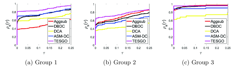
Figure 2: Performance profiles for the accuracy of solutions with $\tau=0.25$.

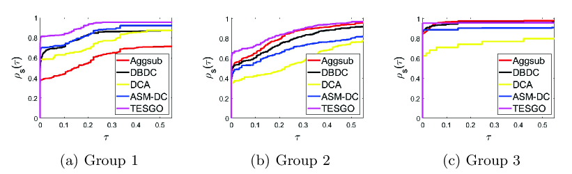
Figure 3: Performance profiles for the accuracy of solutions with $\tau=0.55$.

We can see from Figure 2 that in all three groups the proposed TESGO method outperforms other local methods in finding high quality solutions. Results obtained by local methods using 20 randomly generated starting points show that problems from Groups 1 and 2 have many local minimizers while problems from Group 3 have very few. In the global optimization context, this means problems from Groups 1 and 2 are more difficult than those in Group 3. In Groups 1 and 2, the difference between TESGO and local methods is considerable. In particular, in Group 1 TESGO finds the global minimizers in approximately 82% of problems whereas the best performed local method, ASM-DC, finds such minimizers in approximately 67% of problems. In Group 2, TESGO finds the global minimizers in almost 63% of problems whereas the best performed local method, DBDC, finds such minimizers in 50% of problems. Furthermore, in Groups 1 and 2, TESGO finds $\tau$-approximate global minimizers with $\tau=0.05$ in almost 83% and 70% of problems, respectively, whereas best performed local methods, ASM-DC and AggSub, find such solutions in almost 68% and 58% of problems, respectively. The TESGO method outperforms local methods also in Group 3, however the difference between TESGO and the best performed local method, DBDC is not significant. To conclude, results presented in Figures 2 and 3 show that TESGO is efficient in escaping from local minimizers and in finding high quality solutions using the limited number of $\varepsilon$-subgradients of DC components.

Next, we present performance profiles using CPU time and the number of function evaluations and provide a pairwise comparison of TESGO with AggSub, ASM-DC, DBDC and DCA. Since some of the methods use different amount of DC component evaluations, the number of function evaluations for each run of algorithms is calculated as an average of the number of evaluations of the first and second DC components. The number of subgradient evaluations follows the similar trends with the number of the function evaluations with all the solvers, and thus, we omit these results. In addition, only results with $\tau$-approximate global minimizers with the selection $\tau=0.2$ are considered. Recall that in the standard performance profiles, the value of $\rho_{s}(\tau)$ at $\tau=0$ shows the ratio of the test problems for which the solver $s$ is the best — that is, the solver $s$ uses the least computational time or evaluations — while the value of $\rho_{s}(\tau)$ at the rightmost abscissa gives the ratio of the test problems that the solver $s$ can solve — that is, the robustness of the solver $s$. In addition, the higher is a particular curve, the better is the corresponding solver. Results presented in Figures 4$-$9 clearly show that TESGO is more robust than local methods, used in numerical experiments, across three groups of test problems. The only exception is AggSub which has a similar robustness in Group 3. On the other side, TESGO uses, in general, significantly more CPU time and function evaluations than the other local methods. This is expected as TESGO escapes from local minimizers and applies a local method multiple times.

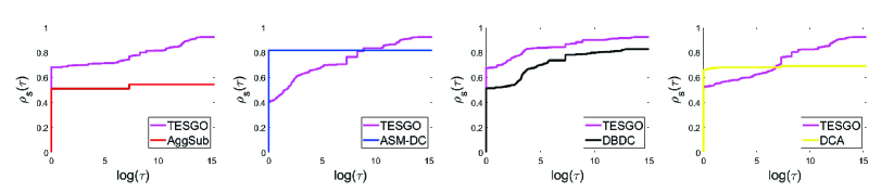
Figure 4: Performance profiles for problems from Group 1 using CPU time.

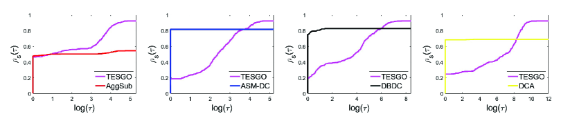
Figure 5: Performance profiles for problems from Group 1 using number of function evaluations.

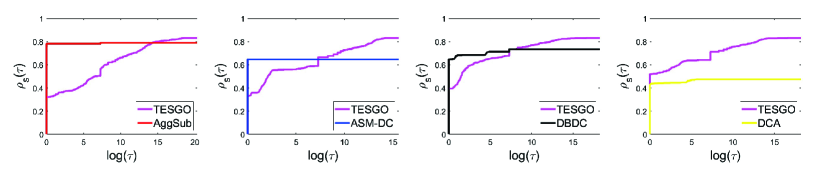
Figure 6: Performance profiles for problems from Group 2 using CPU time.

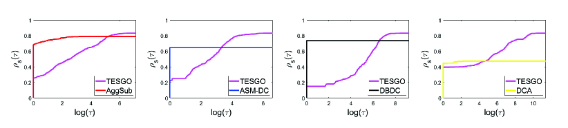
Figure 7: Performance profiles for problems from Group 2 using number of function evaluations.

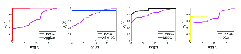
Figure 8: Performance profiles for problems from Group 3 using CPU time.

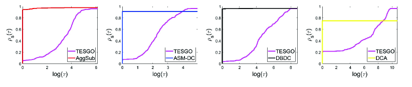
Figure 9: Performance profiles for problems from Group 3 using number of function evaluations.

In addition to performance profiles, we report the number of function and subgradient evaluations of DC components in Tables 2 – 4. In these tables, $n_{f}$ stands for the number of evaluations of the objective function $f$ whereas $n_{f_{i}}$ is the number of function evaluations and $n_{g_{i}}$ is the number of subgradient evaluations of the DC component $f_{i},~i=1,2$. We use the notation $n_{fg_{i}}$ when $n_{f_{i}}=n_{g_{i}},~i=1,2$. In AggSub and DBDC, we only report $n_{f}$ as for them we have $n_{f_{1}}=n_{f_{2}}$. In DCA, $n_{f_{i}}=n_{g_{i}},~i=1,2$ and thus we report the values of $n_{fg_{1}}$ and $n_{fg_{2}}.$ Since we use 20 starting points for each problem, we report the mean value over 20 runs of the methods.

Table 2: Number of function and subgradient evaluations of DC components (Group 1).

Prob.	$n$		AggSub				DBDC				DCA			ASM-DC					TESGO
			$n_{f}$	$n_{g_{1}}$	$n_{g_{2}}$		$n_{f}$	$n_{g_{1}}$	$n_{g_{2}}$		$n_{fg_{1}}$	$n_{fg_{2}}$		$n_{f_{1}}$	$n_{f_{2}}$	$n_{g_{1}}$	$n_{g_{2}}$		$n_{f_{1}}$	$n_{f_{2}}$	$n_{g_{1}}$	$n_{g_{2}}$
$P_{1}$	2		199	101	40		94	93	92		37	2		321	211	110	46		350	229	174	77
$P_{2}$	4		4895	4754	89		35	36	32		30	2		630	391	240	71		4240	1932	1924	400
$P_{3}$	2		3748	3634	75		582	581	526		811	56		420	272	148	49		4917	1385	1984	268
$P_{4}$	3		173	121	32		139	139	62		40	3		385	257	128	42		3065	874	1291	180
$P_{5}$	2		127	82	27		59	59	35		6	2		235	155	81	30		1733	606	704	140
$P_{5}$	5		144	94	31		107	108	56		7	2		282	180	103	33		3050	1169	1339	282
$P_{5}$	10		144	90	30		101	102	54		8	2		334	209	126	35		3964	1438	1893	385
$P_{5}$	50		147	89	31		93	94	52		8	2		541	317	224	38		3272	1113	2022	268
$P_{5}$	100		146	98	33		81	82	50		9	3		624	356	268	35		3531	1214	2193	252
$P_{5}$	200		165	119	36		60	61	40		9	3		597	345	252	37		2894	869	1959	224
$P_{6}$	3		4549	4446	64		29	29	24		29	2		348	220	128	41		603	329	309	100
$P_{7}$	2		53	30	20		7	8	8		16	2		135	89	46	23		892	329	371	114
$P_{7}$	5		267	194	33		7864	7863	7862		45	2		590	369	221	56		7722	2239	3169	395
$P_{7}$	10		387	281	43		9529	9527	9524		49	2		1220	757	463	88		13938	4466	5697	635
$P_{7}$	50		767	677	50		10014	10012	10010		59	2		3159	1775	1383	144		22435	5057	10321	533
$P_{7}$	100		1231	1163	52		10016	10012	10010		60	2		6308	3403	2905	201		29482	6198	13918	495
$P_{7}$	200		10868	10080	626		10022	10015	10014		77	2		10851	5740	5111	281		35181	7007	16772	476
$P_{8}$	5		831	792	45		1176	1133	92		9085	3		691	425	267	49		16603	3796	7078	489
$P_{8}$	10		3003	2834	154		2400	2329	238		6245	3		1501	848	654	69		32038	8516	14396	776
$P_{8}$	50		18423	18217	202		7563	7492	1988		109471	9		16343	8369	7975	202		76821	34120	37888	909
$P_{8}$	100		27456	27273	194		30833	30545	21325		70195	9		45771	23142	22630	305		85168	37665	42472	625
$P_{8}$	200		75375	75178	215		5850	5791	5082		404000	20		8918	4581	4337	145		32898	12431	16451	499

Table 3: Number of function and subgradient evaluations of DC components (Group 2).

Prob.	$n$		AggSub				DBDC				DCA			ASM-DC					TESGO
			$n_{f}$	$n_{g_{1}}$	$n_{g_{2}}$		$n_{f}$	$n_{g_{1}}$	$n_{g_{2}}$		$n_{fg_{1}}$	$n_{fg_{2}}$		$n_{f_{1}}$	$n_{f_{2}}$	$n_{g_{1}}$	$n_{g_{2}}$		$n_{f_{1}}$	$n_{f_{2}}$	$n_{g_{1}}$	$n_{g_{2}}$
$P_{9}$	2		409	277	55		42	35	29		39	3		355	236	118	43		4588	797	1962	167
$P_{9}$	5		1141	870	113		76	63	45		116	3		817	524	292	73		10077	2377	4136	393
$P_{9}$	10		2365	1880	188		121	110	76		180	2		1392	851	541	97		13772	3406	6030	488
$P_{9}$	50		10666	9817	304		644	624	200		13606	2		6838	3682	3156	161		22334	9858	11277	467
$P_{9}$	100		20268	19591	268		1589	1561	559		31362	2		14226	7473	6754	209		31013	14248	15613	450
$P_{10}$	2		357	229	53		40	29	24		27	3		350	239	111	43		4901	823	2050	174
$P_{10}$	5		1071	948	84		62	55	44		110	3		825	543	282	76		10594	2704	4344	431
$P_{10}$	10		2374	2129	172		122	115	72		257	3		1604	974	630	114		17969	5025	7817	665
$P_{10}$	50		25614	24782	721		1178	1158	447		4415	3		23120	12029	11091	506		61393	30073	30080	1186
$P_{10}$	100		22809	22398	376		2865	2844	1121		13654	4		83252	42449	40803	1063		97002	47538	48209	1282
$P_{11}$	2		127	82	27		59	59	35		6	2		235	155	81	30		4548	595	2041	142
$P_{11}$	5		144	94	31		107	108	56		7	2		282	180	103	33		7111	1204	3228	297
$P_{11}$	10		144	90	30		101	102	54		8	2		334	209	126	35		8598	1480	4059	410
$P_{11}$	50		147	89	31		93	94	52		8	2		541	317	224	38		7778	1248	4165	295
$P_{11}$	100		146	98	33		81	82	50		9	3		624	356	268	35		7500	1181	4083	266
$P_{11}$	200		165	119	36		60	61	40		9	3		597	345	252	37		7040	869	3928	244
$P_{12}$	2		58	42	18		27	27	13		23	3		112	73	40	18		3428	385	1434	119
$P_{12}$	5		304	256	40		71	70	37		48	3		426	262	164	35		10736	1688	4510	301
$P_{12}$	10		427	348	59		132	131	76		80	3		1079	627	451	64		16267	4092	7323	546
$P_{12}$	50		3605	3382	204		241	240	157		150	3		2611	1381	1230	76		17738	3904	8927	383
$P_{12}$	100		2255	2092	155		268	269	184		232	3		3861	2006	1854	77		19525	5250	9900	346
$P_{12}$	200		2438	2275	161		497	495	366		350	3		3758	1964	1793	87		17479	3969	8868	333
$P_{13}$	2		243	208	30		32	32	17		24	3		223	138	85	25		5209	764	2190	174
$P_{13}$	5		755	676	63		101	102	63		73	4		451	283	167	31		16732	1926	7233	335
$P_{13}$	10		1465	1357	89		204	205	148		92	4		703	405	298	42		26730	3811	12255	714
$P_{13}$	50		2401	2277	108		443	444	358		182	4		1344	712	632	35		25503	4475	12963	521
$P_{13}$	100		3120	2995	123		389	389	301		261	4		2257	1172	1086	39		29193	6021	14993	512
$P_{13}$	200		5080	4953	129		485	486	351		389	4		2247	1168	1078	41		27111	5128	13753	487
$P_{14}$	2		228	205	27		27	19	16		31	2		297	185	112	30		1244	469	553	103
$P_{14}$	5		550	499	51		49	38	26		63	2		654	419	235	43		987	533	513	128
$P_{14}$	10		1182	1065	98		107	95	55		109	2		1075	637	438	51		1613	843	953	213
$P_{14}$	50		9765	9509	246		714	701	333		2791	2		4440	2334	2106	70		23681	10507	12094	416
$P_{14}$	100		46252	45820	436		3159	3143	1674		8770	2		6843	3520	3323	118		27344	12028	14018	511
$P_{14}$	200		69437	69109	325		3869	3854	2834		71000	4		6912	3573	3339	132		18789	7686	9767	426

Table 4: Number of function and subgradient evaluations of DC components (Group 3).

Prob.	$n$		AggSub				DBDC				DCA			ASM-DC					TESGO
			$n_{f}$	$n_{g_{1}}$	$n_{g_{2}}$		$n_{f}$	$n_{g_{1}}$	$n_{g_{2}}$		$n_{fg_{1}}$	$n_{fg_{2}}$		$n_{f_{1}}$	$n_{f_{2}}$	$n_{g_{1}}$	$n_{g_{2}}$		$n_{f_{1}}$	$n_{f_{2}}$	$n_{g_{1}}$	$n_{g_{2}}$
$P_{15}$	2		141	103	29		70	65	43		101	7		290	191	99	36		3016	1148	1180	237
$P_{16}$	2		111	82	25		23	21	16		5	2		215	135	80	28		1642	774	690	178
$P_{16}$	5		118	83	27		22	22	16		5	2		262	158	104	30		2254	1007	1044	252
$P_{16}$	10		119	82	28		18	18	14		5	2		323	194	130	32		2926	1312	1429	337
$P_{16}$	50		130	87	30		26	25	20		6	2		539	301	238	33		3250	1484	2081	278
$P_{16}$	100		139	99	32		14	15	11		6	2		846	451	395	32		4227	1889	2586	256
$P_{16}$	200		145	109	31		18	19	19		6	2		955	513	442	35		3653	1543	2317	228
$P_{17}$	2		240	153	49		62	50	34		128	9		352	235	116	36		2123	758	845	137
$P_{18}$	2		125	95	25		48	42	28		31	2		274	179	94	34		1003	587	415	133
$P_{18}$	5		172	127	34		147	140	79		46	3		452	286	166	44		1386	768	662	180
$P_{18}$	10		182	135	35		165	160	89		36	3		533	326	207	46		2169	1149	1130	285
$P_{18}$	50		209	140	39		180	181	95		30	3		780	453	327	46		4334	1843	2538	302
$P_{18}$	100		221	159	41		161	162	88		29	3		1038	582	456	47		4320	1786	2584	263
$P_{18}$	200		239	181	43		135	136	79		27	3		1101	627	473	48		3253	1197	2106	213
$P_{19}$	2		122	91	26		56	53	32		5	2		247	158	88	31		1322	584	575	140
$P_{20}$	2		151	111	26		23	14	13		33	3		258	165	93	28		2213	611	936	135
$P_{20}$	5		334	244	60		448	429	287		1087	26		768	479	289	54		15946	3311	6645	419
$P_{20}$	10		3530	2397	758		15720	15660	11668		1404	23		1432	826	606	71		27681	6466	12363	662
$P_{20}$	50		57539	51804	5550		4796	4780	3553		29753	114		16395	8377	8018	253		70158	29780	34564	994
$P_{20}$	100		68127	64597	3491		33580	33563	20919		108401	229		28946	14629	14317	281		95306	42935	47362	927
$P_{20}$	200		107855	105092	2760		12408	12391	9157		396454	89		19377	9828	9549	239		60257	25700	29943	736

Results presented in Tables 2 – 4 show that with very few exceptions TESGO requires significantly more function and subgradient evaluations of both DC components than the other four local methods. As mentioned before, this is due to the fact that TESGO applies the local search method multiple times. However, taking into account that TESGO obtains higher quality solutions than other methods, the computational effort required by this method is reasonable.

7.5 Comparison with global optimization solvers

In this subsection, we present results for global minimization of the test problems from all three groups. The results of the proposed method is also compared with those obtained using well-known global optimization solvers BARON [42] and LINDOGlobal [34]. In addition, we consider two hours time limit for solving each test problem. The results are given in Tables 5$-$7, where we report the optimal value $f_{opt}$ obtained by a solver and errors $E_{T},E_{B}$ and $E_{L}$ computed using (4). The notation $t_{lim}$ in the tables indicates that a solver reach the two hours time limit. Since BARON solver is not applicable to all test problems, we use “–” for such problems in tables. This is due to the fact that BARON cannot handle the maximum function. If the maximum function is used in the first DC component $f_{1}$, then it can be rewritten without the maximum by introducing constraints and one extra variable. This is not possible if the second DC component $f_{2}$ has a maximum function, and thus these types of problems cannot be solved with BARON.

Here we apply the full version of the TESGO method. This means that we compute significantly more $\varepsilon$-subgradients of DC components in comparison with the simple version of TESGO. More specifically, we compute $m_{1}=\min\{100,2n\}$ $\varepsilon$-subgradients of the first DC component and $m_{2}=\min\{30,2n\}$ $\varepsilon$-subgradients of the second DC component. For the test problems with a large number of local minimizers, we set $m_{1}=\min\{150,2n\}$ and $m_{2}=\min\{30,2n\}$ (in tables these problems are indicated by ^∗). Finally, for some very complex problems, we set $m_{1}=\min\{200,2n\}$ and $m_{2}=\min\{30,2n\}$ (in tables these problems are indicated by ^∗∗).

Table 5: Results for TESGO, BARON, and LINDO (Group 1).

Prob.	$n$		TESGO				BARON				LINDO
			$f_{opt}$	$E_{T}$	CPU		$f_{opt}$	$E_{B}$	CPU		$f_{opt}$	$E_{L}$	CPU
$P_{1}$	2		0.0000	0.0000	0.02		0.0000	0.0000	0.05		0.0000	0.0000	0.02
$P_{2}$	4		0.0000	0.0000	0.00		0.0000	0.0000	$t_{lim}$		0.0000	0.0000	0.08
$P_{3}$	2		0.5000	0.0000	0.00		0.5000	0.0000	0.06		0.5000	0.0000	0.13
$P_{4}$	3		3.5000	0.0000	0.00		3.5000	0.0000	0.22		3.5000	0.0000	0.08
$P_{5}$	2		-0.5000	0.0000	0.00		-0.5000	0.0000	0.11		-0.5000	0.0000	0.03
$P_{5}$	5		-3.5000	0.0000	0.20		-3.5000	0.0000	4.17		-3.5000	0.0000	0.09
$P_{5}$	10		-8.5000	0.0000	3.17		-8.5000	0.0000	$t_{lim}$		-8.5000	0.0000	2.31
$P_{5}$	50		-48.5000	0.0000	0.70		-47.5000	0.0202	$t_{lim}$		-48.5000	0.0000	$t_{lim}$
$P_{5}$	100		-98.5000	0.0000	0.77		-90.5000	0.0804	$t_{lim}$		-98.5000	0.0000	$t_{lim}$
$P_{5}$	200		-198.5000	0.0000	0.95		-182.5000	0.0802	$t_{lim}$		-198.5000	0.0000	$t_{lim}$
$P_{6}$	3		116.3333	0.0000	0.00		116.3333	0.0000	0.14		116.3333	0.0000	0.03
$P_{7}$	2		0.0000	0.0000	0.00		0.0000	0.0000	0.04		0.0000	0.0000	0.03
$P_{7}$	5		0.0000	0.0000	0.00		0.0000	0.0000	0.04		0.0000	0.0000	0.22
$P_{7}$	10		0.0000	0.0000	0.02		0.0000	0.0000	0.04		0.0014	0.0014	1.93
$P_{7}$	50		0.0000	0.0000	0.34		0.0000	0.0000	$t_{lim}$		0.0306	0.0306	$t_{lim}$
$P_{7}$	100		0.0000	0.0000	0.86		0.0000	0.0000	0.39		0.0273	0.0273	$t_{lim}$
$P_{7}$	200		0.0000	0.0000	3.97		0.0000	0.0000	2.43		0.0348	0.0348	$t_{lim}$
$P_{8}$	5		0.0000	0.0000	0.08		–	–	–		0.0000	0.0000	263.74
$P_{8}$	10		0.0000	0.0000	0.44		–	–	–		0.0000	0.0000	$t_{lim}$
$P_{8}$	50		0.0000	0.0000	72.17		–	–	–		0.0000	0.0000	4.40
$P_{8}$	100		0.0001	0.0001	1997.05		–	–	–		0.0000	0.0000	3.89
$P_{8}$	200		6.0400∗∗	6.0400∗∗	292.70∗∗		–	–	–		0.0000	0.0000	5.46
∗∗ in TESGO we have set $m_{1}=\min\{200,2n\}$ and $m_{2}=\min\{30,2n\}$

Table 6: Results for TESGO, BARON, and LINDO (Group 2).

Prob.	$n$		TESGO				BARON				LINDO
			$f_{opt}$	$E_{T}$	CPU		$f_{opt}$	$E_{B}$	CPU		$f_{opt}$	$E_{L}$	CPU
$P_{9}$	2		-153.3333	0.0000	0.02		–	–	–		-153.3333	0.0000	376.69
$P_{9}$	5		-436.6667	0.0000	0.03		–	–	–		-436.6667	0.0000	819.50
$P_{9}$	10		-929.0906	0.0000	0.28		–	–	–		-929.0909	0.0000	565.11
$P_{9}$	50		-4921.9601	0.0000	6.00		–	–	–		-4921.7032	0.0001	$t_{lim}$
$P_{9}$	100		-9920.9888∗∗	0.0000∗∗	2219.03∗∗		–	–	–		-9918.9905	0.0002	$t_{lim}$
$P_{10}$	2		-247.8125	0.0000	0.00		-247.8125	0.0000	0.20		-247.8125	0.0000	137.26
$P_{10}$	5		-578.4626	0.0000	0.02		-578.4626	0.0000	0.31		-578.4626	0.0000	198.85
$P_{10}$	10		-1006.8613∗	0.0000∗	0.17∗		-1006.8616	0.0000	0.34		-1006.8616	0.0000	$t_{lim}$
$P_{10}$	50		-3564.2274∗∗	0.0000∗∗	163.52∗∗		-3564.2275	0.0000	1.40		-3538.2191	0.0073	$t_{lim}$
$P_{10}$	100		-7297.9529	0.0000	263.20		-7297.9530	0.0000	5.99		-7235.4972	0.0086	$t_{lim}$
$P_{11}$	2		-0.5000	0.0000	0.00		-0.5000	0.0000	0.12		-0.5000	0.0000	0.04
$P_{11}$	5		-3.5000	0.0000	0.16		-3.5000	0.0000	4.17		-3.5000	0.0000	0.10
$P_{11}$	10		-8.5000	0.0000	0.16		-8.5000	0.0000	5655.25		-8.5000	0.0000	2.47
$P_{11}$	50		-48.5000	0.0000	0.70		-47.5000	0.0202	$t_{lim}$		-48.5000	0.0000	$t_{lim}$
$P_{11}$	100		-98.5000	0.0000	0.78		-89.5000	0.0905	$t_{lim}$		-98.5000	0.0000	$t_{lim}$
$P_{11}$	200		-198.5000	0.0000	0.95		-180.5000	0.0902	$t_{lim}$		-198.5000	0.0000	$t_{lim}$
$P_{12}$	2		0.0000	0.0000	0.00		–	–	–		0.0000	0.0000	0.21
$P_{12}$	5		-1.8541	0.0000	0.05		–	–	–		-1.8541	0.0000	22.18
$P_{12}$	10		-4.9443	0.0000	0.97		–	–	–		-4.9443	0.0000	$t_{lim}$
$P_{12}$	50		-29.6656∗	0.0000∗	3.41∗		–	–	–		-29.6656	0.0000	$t_{lim}$
$P_{12}$	100		-60.5673∗∗	0.0000∗∗	579.05∗∗		–	–	–		-60.5673	0.0000	$t_{lim}$
$P_{12}$	200		-122.3707∗	0.0000∗	42.17∗		–	–	–		-122.3707	0.0000	$t_{lim}$
$P_{13}$	2		-5.0000	0.0000	0.61		–	–	–		-5.0000	0.0000	0.14
$P_{13}$	5		-21.8541	0.0000	0.05		–	–	–		-21.8541	0.0000	1.66
$P_{13}$	10		-48.9443	0.0196	0.08		–	–	–		-49.9443	0.0000	$t_{lim}$
$P_{13}$	50		-226.0525∗∗	0.1733∗∗	31.13∗∗		–	–	–		-273.6652	0.0000	$t_{lim}$
$P_{13}$	100		-555.5672∗∗	0.0000∗∗	560.44∗∗		–	–	–		-554.5672	0.0018	$t_{lim}$
$P_{13}$	200		-939.2915∗∗	0.1584∗∗	195.28∗∗		–	–	–		-1116.3273	0.0000	$t_{lim}$
$P_{14}$	2		-1.0000	0.0000	0.00		–	–	–		-1.0000	0.0000	0.34
$P_{14}$	5		-3.4167	0.0000	0.00		–	–	–		-3.4167	0.0000	15.60
$P_{14}$	10		-11.2897	0.0000	0.03		–	–	–		-11.2897	0.0000	127.92
$P_{14}$	50		-126.9603	0.0000	6.50		–	–	–		-125.8108	0.0090	$t_{lim}$
$P_{14}$	100		-320.7221	0.0000	31.81		–	–	–		-311.7939	0.0278	$t_{lim}$
$P_{14}$	200		-776.3854	0.0016	25.84		–	–	–		-774.7685	0.0036	$t_{lim}$
∗ in TESGO we have set $m_{1}=\min\{150,2n\}$ and $m_{2}=\min\{30,2n\}$
∗∗ in TESGO we have set $m_{1}=\min\{200,2n\}$ and $m_{2}=\min\{30,2n\}$

Table 7: Results for TESGO, BARON, and LINDO (Group 3).

Prob.	$n$		TESGO				BARON				LINDO
			$f_{opt}$	$E_{T}$	CPU		$f_{opt}$	$E_{B}$	CPU		$f_{opt}$	$E_{L}$	CPU
$P_{15}$	2		-0.3524	0.0000	0.00		-0.3524	0.0000	0.06		-0.3524	0.0000	0.48
$P_{16}$	2		0.0000	0.0000	0.02		0.0000	0.0000	0.16		0.0000	0.0000	0.04
$P_{16}$	5		0.0000	0.0000	0.00		0.0000	0.0000	2.73		0.0000	0.0000	0.11
$P_{16}$	10		0.0000	0.0000	0.02		0.0000	0.0000	289.58		0.0000	0.0000	0.16
$P_{16}$	50		0.0000	0.0000	0.58		0.0000	0.0000	$t_{lim}$		0.0000	0.0000	$t_{lim}$
$P_{16}$	100		0.0000	0.0000	0.94		0.0000	0.0000	$t_{lim}$		0.0000	0.0000	$t_{lim}$
$P_{16}$	200		0.0000	0.0000	1.20		0.0000	0.0000	$t_{lim}$		0.0000	0.0000	$t_{lim}$
$P_{17}$	2		-0.8333	0.0000	0.00		-0.8333	0.0000	0.18		-0.8333	0.0000	3.13
$P_{18}$	2		-0.3750	0.0000	0.00		-0.3750	0.0000	0.12		-0.3750	0.0000	0.05
$P_{18}$	5		-1.3750	0.0000	0.00		-1.3750	0.0000	2.10		-1.3750	0.0000	0.12
$P_{18}$	10		-3.0417	0.0000	0.02		-3.0417	0.0000	668.42		-3.0417	0.0000	3.02
$P_{18}$	50		-16.3750	0.0000	0.75		-16.3750	0.0000	$t_{lim}$		-16.3750	0.0000	$t_{lim}$
$P_{18}$	100		-33.0417	0.0000	0.86		-33.0417	0.0000	$t_{lim}$		-33.0417	0.0000	$t_{lim}$
$P_{18}$	200		-66.3750	0.0000	0.95		-66.3750	0.0000	$t_{lim}$		-66.3750	0.0000	$t_{lim}$
$P_{19}$	2		-0.2500	0.0000	0.00		-0.2500	0.0000	0.11		-0.2500	0.0000	0.04
$P_{20}$	2		0.0000	0.0000	0.00		0.0000	0.0000	0.04		0.0000	0.0000	0.08
$P_{20}$	5		0.0000	0.0000	0.06		0.0000	0.0000	0.05		0.0000	0.0000	0.06
$P_{20}$	10		0.0000	0.0000	0.17		0.0000	0.0000	0.04		0.0000	0.0000	0.11
$P_{20}$	50		0.0000	0.0000	7.88		0.0000	0.0000	0.06		0.0000	0.0000	2.08
$P_{20}$	100		0.0000	0.0000	162.97		0.0000	0.0000	0.21		0.0000	0.0000	5.52
$P_{20}$	200		0.0000	0.0000	76.59		0.0000	0.0000	0.64		0.0000	0.0000	16.40

Results from Tables 5$-$7 show that TESGO finds global solutions in 72 cases out of 77, the BARON solver in 43 cases out of 49 and the LINDOGlobal solver in 71 cases out of 77. However, both BARON and LINDOGlobal require significantly more CPU time than TESGO. The only exceptions are $P_{8}$ and $P_{20}$ with $n=50,100,200$. In many cases, BARON and LINDOGlobal are forced to stop due to the two hours time limit. These results clearly indicate that, in general, TESGO is able to find accurate solutions to most DC optimization problems by using significantly less computational effort than BARON and LINDOGlobal.

Finally, in Table 8, we report the number of function and subgradient evaluations required by TESGO to solve DC optimization problems to global optimality. These numbers are computed as an average of the number of function and subgradient evaluations of DC components. We only report these results for TESGO as such information for BARON and LINDOGlobal cannot be extracted. We can see from this table that in most cases the TESGO method uses a reasonable number of function and subgradient evaluations. Depending on the starting point, the large number of local minimizers can lead to large number of function and subgradient evaluations. Problems $P_{8}$ with $n=50,100,200$, $P_{9}$ with $n=100$, $P_{10}$ with $n=50,100$, $P_{12}$ with $n=100$ and $P_{13}$ with $n=50,100,200$ are among such problems. In these problems, TESGO requires a large number of function and subgradient evaluations.

Table 8: Number of function and subgradient evaluations for TESGO

Prob.	$n$	$n_{f}$	$n_{g}$		Prob.	$n$	$n_{f}$	$n_{g}$		Prob.	$n$	$n_{f}$	$n_{g}$
Group 1
$P_{1}$	2	225	159		$P_{5}$	100	3727	1997		$P_{7}$	200	9880	4537
$P_{2}$	4	3631	1452		$P_{5}$	200	4133	2094		$P_{8}$	5	29000	10147
$P_{3}$	2	8428	2767		$P_{6}$	3	266	196		$P_{8}$	10	66402	23332
$P_{4}$	3	1983	771		$P_{7}$	2	1257	532		$P_{8}$	50	147519	50830
$P_{5}$	2	2381	855		$P_{7}$	5	5791	2043		$P_{8}$	100	140322	49153
$P_{5}$	5	3239	1389		$P_{7}$	10	9917	3728		$P_{8}$	200	102488∗∗	39073∗∗
$P_{5}$	10	4806	1991		$P_{7}$	50	9655	4442
$P_{5}$	50	3420	1883		$P_{7}$	100	7243	3521
Group 2
$P_{9}$	2	3701	2432		$P_{11}$	10	4646	3632		$P_{13}$	10	14626	9409
$P_{9}$	5	13261	9196		$P_{11}$	50	2593	2240		$P_{13}$	50	107211∗∗	93647∗∗
$P_{9}$	10	12234	7364		$P_{11}$	100	2968	2656		$P_{13}$	100	135975∗∗	115026∗∗
$P_{9}$	50	13273	12370		$P_{11}$	200	3183	2981		$P_{13}$	200	69674∗∗	55864∗∗
$P_{9}$	100	325787∗∗	324040∗∗		$P_{12}$	2	2260	1443		$P_{14}$	2	337	364
$P_{10}$	2	3444	2319		$P_{12}$	5	11406	7401		$P_{14}$	5	353	478
$P_{10}$	5	8177	5808		$P_{12}$	10	17760	12918		$P_{14}$	10	511	761
$P_{10}$	10	25962∗	17849∗		$P_{12}$	50	28432∗	17843∗		$P_{14}$	50	13300	12397
$P_{10}$	50	330857∗∗	329517∗∗		$P_{12}$	100	110911∗∗	96628∗∗		$P_{14}$	100	13216	11688
$P_{10}$	100	62905	61873		$P_{12}$	200	32535∗	20883∗		$P_{14}$	200	10735	9685
$P_{11}$	2	1969	1589		$P_{13}$	2	4589	2952
$P_{11}$	5	2916	2026		$P_{13}$	5	13040	8531
Group 3
$P_{15}$	2	5151	1780		$P_{17}$	2	1209	428		$P_{19}$	2	719	304
$P_{16}$	2	2172	787		$P_{18}$	2	408	194		$P_{20}$	2	565	282
$P_{16}$	5	981	518		$P_{18}$	5	1515	627		$P_{20}$	5	15638	6023
$P_{16}$	10	3802	1606		$P_{18}$	10	4791	1876		$P_{20}$	10	27899	10966
$P_{16}$	50	3122	1733		$P_{18}$	50	3357	1901		$P_{20}$	50	41399	16070
$P_{16}$	100	2951	1804		$P_{18}$	100	3101	1827		$P_{20}$	100	76660	27748
$P_{16}$	200	4009	2052		$P_{18}$	200	2350	1593		$P_{20}$	200	49536	18500
∗ in TESGO we have set $m_{1}=\min\{150,2n\}$ and $m_{2}=\min\{30,2n\}$
∗∗ in TESGO we have set $m_{1}=\min\{200,2n\}$ and $m_{2}=\min\{30,2n\}$

8 Conclusions

In this paper, a new algorithm, the truncated $\varepsilon$-subdifferential method, is developed to globally minimize DC functions subject to box-constraints. It is a hybrid method based on the combination of a local search and a special procedure for escaping from solutions of a DC function which are not global minimizers. A local search method is applied to find a stationary point (in our case a critical point) of the DC optimization problem. Then the escaping procedure is employed to escape from this point by finding a better initial point for a local search.

We compute subsets of the $\varepsilon$-subdifferentials of DC components. Then we calculate the deviation of the subset of the $\varepsilon$-subdifferential of the second DC component from the subset of the $\varepsilon$-subdifferential of the first DC component. If this deviation is positive then we utilize the $\varepsilon$-subgradient of the second DC component providing this deviation to formulate a subproblem with a convex objective function. The solution to this subproblem is used as a starting point for a local search. The convergence of the conceptual version of the proposed method is studied and its implementation is discussed in detail.

The performance of the new method is demonstrated using a large number of academic test problems for DC optimization. Based on extensive numerical results it is shown that the proposed method is able to significantly improve the quality of solutions obtained by a local method using limited computational effort. In addition, we apply the developed method to find global solutions to DC optimization problems. Results show that the new method is able to find global solutions by increasing the number of $\varepsilon$-subgradients calculations in the escaping procedure. Comparison with two widely used global optimization solvers shows that the proposed method is efficient and accurate for solving DC optimization problems to global optimality using significantly less computational effort.

Statements and Declarations

Appendix: Test problems

All objective functions are DC functions:

$$f({\bm{x}})=f_{1}({\bm{x}})-f_{2}({\bm{x}})$$

Problem 1

DC version of Aluffi-Pentini’s problem

$$f_{1}({\bm{x}})=0.25x_{1}^{4}+0.1x_{1}+0.5x_{2}^{2},~~~~f_{2}({\bm{x}})=0.5x_{1}^{2}$$

$${\bm{x}}=(x_{1},x_{2})\in\mathbb{R}^{2},~~x_{i}\in[-10,10],~i=1,2.$$

Problem 2

Generalized DC Becker and Lago problem

$$f_{1}({\bm{x}})=\sum_{i=1}^{n}x_{i}^{2}+25n,~~~~f_{2}({\bm{x}})=10\sum_{i=1}^{n}|x_{i}|$$

$${\bm{x}}\in\mathbb{R}^{n},~~x_{i}\in[-10,10],~i=1,\ldots,n.$$

Problem 3

Modified DC Camel Back problem

$$f_{1}({\bm{x}})=\frac{1}{6}+x_{1}^{6}+4x_{1}^{2}+4x_{2}^{4}+|x_{1}|,~~~~f_{2}({\bm{x}})=2.1x_{1}^{4}+4x_{2}^{2}$$

$${\bm{x}}=(x_{1},x_{2})\in\mathbb{R}^{2},~~x_{i}\in[-5,5],~i=1,2.$$

Problem 4

$$f_{1}({\bm{x}})=\sum_{i=2}^{n}\big{(}(x_{i}-1)^{2}+x_{i-1}^{2}+x_{i}^{2}\big{)},~~~~f_{2}({\bm{x}})=\sum_{i=2}^{n}|x_{i-1}+x_{i}|$$

$${\bm{x}}\in\mathbb{R}^{n},~~x_{i}\in[-n,n],~i=1,\ldots,n.$$

Problem 5

$$f_{1}({\bm{x}})=2(x_{1}^{2}+x_{2}^{2}),~~~~f_{2}({\bm{x}})=|x_{1}+x_{2}|$$

$${\bm{x}}\in\mathbb{R}^{2},~~x_{i}\in[-10,10],~i=1,2.$$

Problem 6

$$f_{1}({\bm{x}})=2\sum_{i=1}^{n-1}\max\Big{\{}x_{i+1}-x_{i}+1,x_{i}^{2}\Big{\}},~~~f_{2}({\bm{x}})=\sum_{i=1}^{n-1}\Big{(}x_{i}^{2}+x_{i+1}-x_{i}+1\Big{)}$$

$${\bm{x}}\in\mathbb{R}^{n},~~x_{i}\in[-10,10],~i=1,\ldots,n.$$

References

- [1] Ackooij, W., Demassey, S., Javal, P., Morais, H., de Oliveira, W., Swaminathan, B.: A bundle method for nonsmooth DC programming with application to chance-constrained problems. Comput. Optim. Appl. 78(1), 451–490 (2021). DOI https://doi.org/10.1007/s10589-020-00241-8
- [2] An, L.T.H., Tao, P.D.: The DC (difference of convex functions) programming and DCA revisited with DC models of real world nonconvex optimization problems. Ann. Oper. Res. 133, 23–46 (2005). DOI https://doi.org/10.1007/s10479-004-5022-1
- [3] An, L.T.H., Tao, P.D., Ngai, H.V.: Exact penalty and error bounds in DC programming. J. Glob. Optim. 52(3), 509–535 (2012). DOI https://doi.org/10.1007/s10898-011-9765-3
- [4] Artacho, F.J.A., Campoy, R., Vuong, P.T.: Using positive spanning sets to achieve -stationarity with the boosted DC algorithm. Vietnam J. Math. 48(2), 363–376 (2020). DOI https://doi.org/10.1007/s10013-020-00400-8
- [5] Artacho, F.J.A., Fleming, R.M.T., Vuong, P.T.: Accelerating the DC algorithm for smooth functions. Math. Program. 169, 95–118 (2018). DOI https://doi.org/10.1007/s10107-017-1180-1
- [6] Artacho, F.J.A., Vuong, P.T.: The boosted difference of convex functions algorithm for nonsmooth functions. SIAM J. Optim. 30(1), 980–1006 (2020). DOI https://doi.org/10.1137/18M123339X
- [7] Bagirov, A.M., Hoseini Monjezi, N., Taheri, S.: An augmented subgradient method for minimizing nonsmooth DC functions. Comput. Optim. Appl. 80(1), 411–438 (2021). DOI https://doi.org/10.1007/s10589-021-00304-4
- [8] Bagirov, A.M., Karmitsa, N., Mäkelä, M.M.: Introduction to Nonsmooth Optimization. Springer, Cham (2014). DOI https://doi.org/10.1007/978-3-319-08114-4
- [9] Bagirov, A.M., Karmitsa, N., Taheri, S.: Partitional Clustering via Nonsmooth Optimization. Springer, Cham (2020). DOI https://doi.org/10.1007/978-3-030-37826-4
- [10] Bagirov, A.M., Taheri, S., Cimen, E.: Incremental DC optimization algorithm for large-scale clusterwise linear regression. J. Comput. Appl. Math 389, 113323 (2021). DOI https://doi.org/10.1016/j.cam.2020.113323
- [11] Bagirov, A.M., Taheri, S., Joki, K., Karmitsa, N., Mäkelä, M.M.: A new subgradient based method for nonsmooth DC programming, TUCS. Tech. rep., No. 1201, Turku Centre for Computer Science, Turku (2019)
- [12] Bagirov, A.M., Taheri, S., Joki, K., Karmitsa, N., Mäkelä, M.M.: Aggregate subgradient method for nonsmooth DC optimization. Optim. Lett. 15(1), 83–96 (2021). DOI https://doi.org/10.1007/s11590-020-01586-z
- [13] Bagirov, A.M., Taheri, S., Ugon, J.: Nonsmooth DC programming approach to the minimum sum-of-squares clustering problems. Pattern Recognit. 53, 12–24 (2016). DOI https://doi.org/10.1016/j.patcog.2015.11.011
- [14] Bagirov, A.M., Ugon, J.: Codifferential method for minimizing nonsmooth DC functions. J. Glob. Optim. 50, 3–22 (2011). DOI https://doi.org/10.1007/s10898-010-9569-x
- [15] Clarke, F.H.: Optimization and Nonsmooth Analysis. Wiley-Interscience, New York (1983)
- [16] Czyzyk, J., Mesnier, M.P., Moré, J.J.: The NEOS Server. IEEE Comput. Sci. Eng. 5(3), 68–75 (1998). DOI https://doi.org/10.1109/99.714603
- [17] Demyanov, V.F., Vasilyev, L.: Nondifferentiable Optimization. Optimization Software, New York (1986)
- [18] Dolan, E.D.: The NEOS Server 4.0 administrative guide. Technical Memorandum ANL/MCS-TM-250, Mathematics and Computer Science Division, Argonne National Laboratory (2001)
- [19] Dolgopolik, M.V.: A convergence analysis of the method of codifferential descent. Comput. Optim. Appl. 71(1), 879–913 (2018). DOI https://doi.org/10.1007/s10589-018-0024-0
- [20] Ferrer, A., Bagirov, A.M., Beliakov, G.: Solving DC programs using the cutting angle method. J. Glob. Optim. 61, 71–89 (2015). DOI https://doi.org/10.1007/s10898-014-0159-1
- [21] Frangioni, A.: Solving semidefinite quadratic problems within nonsmooth optimization algorithms. Computers & Oper. Res. 23(11), 1099–1118 (1996). DOI https://doi.org/10.1016/0305-0548(96)00006-8
- [22] Gaudioso, M., Giallombardo, G., Miglionico, G., Bagirov, A.M.: Minimizing nonsmooth DC functions via successive DC piecewise-affine approximations. J. Glob. Optim. 71(1), 37–55 (2018). DOI https://doi.org/10.1007/s10898-017-0568-z
- [23] Goldstein, A.A.: Optimization of lipschitz continuous functions. Math. Program. 13, 14–22 (1977). DOI https://doi.org/10.1007/BF01584320
- [24] Gropp, W., Moré, J.J.: Optimization environments and the NEOS Server. In: M.D. Buhman, A. Iserles (eds.) Approximation Theory and Optimization, pp. 167–182. Cambridge University Press (1997)
- [25] Hiriart-Urruty, J.B.: From convex optimization to nonconvex optimization. Necessary and sufficient conditions for global optimality. In: F.H. Clarke, V.F. Dem’yanov, F. Giannessi (eds.) Nonsmooth Optimization and Related Topics, Ettore Majorana International Sciences Series 43, pp. 219–239. Springer, Boston (1989)
- [26] Horst, R., Pardalos, P.M., Thoai, N.V.: Introduction to Global Optimization. Kluwer Academic Publishers, Dordrecht (1995)
- [27] Horst, R., Thoai, N.V.: DC programming: Overview. J. Optim. Theory Appl. 103(1), 1–43 (1999). DOI https://doi.org/10.1023/A:1021765131316
- [28] Horst, R., Thoai, N.V., Benson, H.P.: Concave minimization via conical partitions and polyhedral outer approximation. Math. Program. 50, 259–274 (1991). DOI https://doi.org/10.1007/BF01594938
- [29] Horst, R., Thoai, N.V., Tuy, H.: Outer approximation by polyhedral convex sets. Oper.-Res.-Spektrum 9, 153–159 (1987). DOI https://doi.org/10.1007/BF01721096
- [30] Horst, R., Tuy, H.: Global Optimization (Deterministic Approach). Springer Verlag, Berlin, Germany (1996)
- [31] Joki, K., Bagirov, A.M., Karmitsa, N., Mäkelä, M.M.: A proximal bundle method for nonsmooth DC optimization utilizing nonconvex cutting planes. J. Glob. Optim. 68(1), 501–535 (2017). DOI https://doi.org/10.1007/s10898-016-0488-3
- [32] Joki, K., Bagirov, A.M., Karmitsa, N., Mäkelä, M.M., Taheri, S.: Double bundle method for finding Clarke stationary points in nonsmooth DC programming. SIAM J. Optim. 28(2), 1892–1919 (2018). DOI https://doi.org/10.1137/16M1115733
- [33] Kiwiel, K.C.: A dual method for certain positive semidefinite quadratic programming problems. SIAM J. Sci. Stat. Comput. 10(1), 175–186 (1989). DOI https://doi.org/10.1137/0910013
- [34] Lin, Y., Schrage, L.: The global solver in the LINDO API. Optim. Methods Softw. 24(4-5), 657–668 (2009). DOI https://doi.org/10.1080/10556780902753221
- [35] Mäkelä, M.M., Neittaanmäki, P.: Nonsmooth Optimization: Analysis and Algorithms with Applications to Optimal Control. World Scientific Publishing Co, Singapore (1992)
- [36] Moré, J., Dolan, E.: Benchmarking optimization software with performance profiles. Math. Program. 91, 201–213 (2002). DOI https://doi.org/10.1007/s101070100263
- [37] Nurminski, E.A.: Projection onto polyhedra in outer representation. Comput. Math. & Math. Phys. 48(3), 367–375 (2008). DOI https://doi.org/10.1134/S0965542508030044
- [38] de Oliveira, W.: Proximal bundle methods for nonsmooth DC programming. J. Glob. Optim. 75, 523–563 (2019). DOI https://doi.org/10.1007/s10898-019-00755-4
- [39] de Oliveira, W.: The ABC of DC programming. Set-Valued Var. Anal. 28(1), 679–706 (2020). DOI https://doi.org/10.1007/s11228-020-00566-w
- [40] Pinter, J.: Global Optimization in Action. Kluwer Academic Publishers, Dordrecht (1996)
- [41] Rockafellar, R.T.: Convex Analysis. Princeton University Press, Princeton (1970)
- [42] Sahinidis, N.V.: BARON 23.5.23: Global Optimization of Mixed-Integer Nonlinear Programs, User’s Manual (2023)
- [43] Tuy, H.: Convex Analysis and Global Optimization. Kluwer Academic Publishers, Dordrecht (1998)
- [44] Wolfe, P.H.: Finding the nearest point in a polytope. Math. Program. 11(2), 128–149 (1976). DOI https://doi.org/10.1007/BF01580381