Adaptive Numerical Differentiation
for Extremum Seeking with Sensor Noise

Abstract

Extremum-seeking control (ESC) is widely used to optimize performance when the system dynamics are uncertain. However, sensitivity to sensor noise is an important issue in ESC implementation due to the use of high-pass filters or gradient estimators. To reduce the sensitivity of ESC to noise, this paper investigates the use of adaptive input and state estimation (AISE) for numerical differentiation. In particular, this paper develops extremum-seeking control with adaptive input and state estimation (ESC/AISE), where the high-pass filter of ESC is replaced by AISE to improve performance under sensor noise. The effectiveness of ESC/AISE is illustrated via numerical examples.

I Introduction

Extremum-seeking control (ESC) is used to optimize a performance variable under conditions of high modeling uncertainty. ESC offers theoretical guarantees for convergence to a neighborhood of an optimizer under well-understood conditions [1, 2]. Applications of ESC include robotics [3, 4], energy management [5, 6], combustion [7, 8], and nuclear fusion [9, 10].

Despite these successes, ESC possesses performance limitations relating to stability, changes in the operating point, and other issues [11]. To improve the performance of ESC, various modifications have been implemented [12, 13, 14, 15, 16, 17, 18, 19, 20]. In particular, modifications have been implemented to mitigate the sensitivity to sensor noise [21, 22, 23, 24, 25, 26, 27, 28, 29, 30, 31]. Sensor noise remains an important issue in ESC implementation, especially due to the use of high-pass filters or gradient estimators.

The contribution of the present paper is a variation of ESC that improves optimization performance under sensor noise. In particular, we consider discrete-time ESC, where the high-pass filter is replaced by adaptive input and state estimation (AISE), which provides real-time numerical differentiation in the presence of sensor noise [32, 33, 34]. The application of AISE to ESC comprises extremum-seeking control with adaptive input and state estimation (ESC/AISE). For simplicity, ESC/AISE in this paper is limited to the SISO case.

The contents of the paper are as follows. Section II provides a statement of the control problem, which involves continuous-time dynamics under sampled-data feedback control. Section III provides a review of discrete-time ESC. Section IV introduces ESC/AISE, where the high-pass filter in ESC is replaced by AISE. Section V presents examples that illustrate the performance of ESC/AISE when sensor noise is added to the system output and compares it against discrete-time ESC. Finally, Section VI presents conclusions.

Notation: ${\mathbb{R}}\stackrel{{\scriptstyle\triangle}}{{=}}(-\infty,$ $\infty),$ ${\mathbb{C}}$ denotes the complex numbers, $\|\cdot\|$ denotes the Euclidean norm on ${\mathbb{C}}^{n},$ and ${\bf z}\in{\mathbb{C}}$ denotes the Z-transform variable. $I_{n}$ denotes an $n\times n$ identity matrix. $\lfloor\cdot\rfloor$ denotes the floor function. For all $x\in{\mathbb{R}}$ and $\varepsilon>0,$ ${\mathbb{B}}_{\varepsilon}(x)$ denotes the open ball of radius $\varepsilon$ centered at $x$.

II Problem Statement

We consider continuous-time dynamics under sampled-data control using discrete-time control to reflect the practical implementation of digital controllers for physical systems. In particular, we consider the control architecture in Figure 1, where $M$ is the target continuous-time system, for all $t\geq 0$, $u(t)\in{\mathbb{R}}$ is the control, $y(t)\in{\mathbb{R}}$ is the output of $M,$ and $v(t)\in{\mathbb{R}}$ is the sensor noise.

The output $y(t)$ and the sensor noise $v(t)$ are sampled to generate the sampled noisy measurement $y_{{\rm n},k}\in{\mathbb{R}},$ which, for all $k\geq 0,$ is given by

$$v_{k} \stackrel{{\scriptstyle\triangle}}{{=}}v(kT_{\rm s}),$$ (1)

$$y_{{\rm n},k} \stackrel{{\scriptstyle\triangle}}{{=}}y(kT_{\rm s})+v(kT_{\rm s})=y_{k}+v_{k},$$ (2)

where $T_{\rm s}>0$ is the sampling time. The discrete-time controller is denoted by $G_{\rm c}$. The input to $G_{\rm c}$ is $y_{{\rm n},k}$, and its output at each step $k$ is the discrete-time control $u_{k}\in{\mathbb{R}}.$ The continuous-time control $u(t)$ applied to the structure is generated by applying a zero-order-hold operation to $u_{k},$ that is, for all $k\geq 0,$ and, for all $t\in[kT_{\rm s},(k+1)T_{\rm s}),$

$$u(t)=u_{k}.$$ (3)

Let $\mathcal{U}_{\rm min}\subseteq{\mathbb{R}}$ be the set of values of $u$ that locally minimize $y,$ and let $\mathcal{U}_{\rm max}\subseteq{\mathbb{R}}$ be the set of values of $u$ that locally maximize $y.$ Note that $u$ locally minimizes $y$ if and only if $u$ locally maximizes $-y$. We assume that $\mathcal{U}_{\rm min}$ and $\mathcal{U}_{\rm max}$ have no accumulation points. The objective of the discrete-time controller is to provide an input $u(t)$ such that the output $y(t)$ converges to a neighborhood of either a local minimizer or a local maximizer. When the objective is minimization, the objective is to obtain $u(t)$ such that there exist $\varepsilon>0,$ $t_{\rm c}>0,$ and $u_{\rm min}^{\star}\in\mathcal{U}_{\rm min}$ such that ${\mathbb{B}}_{\varepsilon}(u_{\rm min}^{\star})\cap\mathcal{U}_{\rm min}=\{u_{\rm min}^{\star}\}$ and, for all $t\geq t_{\rm c},$ $u(t)\in{\mathbb{B}}_{\varepsilon}(u_{\rm min}^{\star}).$ When the objective is maximization, the objective is to obtain $u(t)$ such that there exist $\varepsilon>0,$ $t_{\rm c}>0,$ and $u_{\rm max}^{\star}\in\mathcal{U}_{\rm max}$ such that ${\mathbb{B}}_{\varepsilon}(u_{\rm max}^{\star})\cap\mathcal{U}_{\rm max}=\{u_{\rm max}^{\star}\}$ and, for all $t\geq t_{\rm c},$ $u(t)\in{\mathbb{B}}_{\varepsilon}(u_{\rm max}^{\star}).$

Figure 1: Sampled-data implementation of the discrete-time controller $G_{\rm c}$ for controlling the continuous-time system $M$ with input $u,$ output $y,$ and sensor noise $v.$ All sample-and-hold operations are synchronous, and the sampling time is given by $T_{\rm s}>0.$ The discrete-time controller uses the sampled noisy measurement $y_{{\rm n},k}\stackrel{{\scriptstyle\triangle}}{{=}}y(kT_{\rm s})+v(kT_{\rm s})$ as the input and generates the discrete-time control $u_{k}$ at each step $k$. The resulting continuous-time control $u(t)$ is generated by applying a zero-order-hold operation to $u_{k}$. The objective of the controller is to provide an input $u(t)$ that converges to a neighborhood of an input value that either locally minimizes or locally maximizes the output $y(t).$

III Overview of Discrete-Time Extremum-seeking control

For all $k\geq 1,$ the update equations for discrete-time ESC are given by

$$y_{{\rm h},k} =-\omega_{\rm h}T_{\rm s}y_{{\rm h},k-1}+y_{{\rm g},k}-y_{{\rm g},k-1},$$ (4)

$$y_{{\rm l},k} =(1-\omega_{\rm l}T_{\rm s})y_{{\rm l},k-1}$$

$$\quad+\omega_{\rm l}T_{\rm s}K_{{\rm en},k}y_{{\rm h},k-1}A_{\rm esc}\sin{(\omega_{\rm esc}T_{\rm s}(k-1))},$$ (5)

$$y_{{\rm esc},k} =y_{{\rm esc},k-1}+y_{{\rm l},k-1},$$ (6)

$$u_{k} =K_{\rm esc}y_{{\rm esc},k}+A_{\rm esc}\sin{(\omega_{\rm esc}T_{\rm s}k)}+\omega_{0},$$ (7)

where $y_{{\rm g},k}\stackrel{{\scriptstyle\triangle}}{{=}}K_{\rm g}y_{{\rm n},k},$ $K_{\rm g}>0$ is a scaling gain, $y_{{\rm h},k},$ $y_{{\rm l},k},$ $y_{{\rm esc},k}\in{\mathbb{R}}$ are internal states, $K_{{\rm en},k}\in\{0,1\}$ is an enabling gain, $K_{\rm esc}$ is the ESC output gain, $\omega_{\rm l}>0$ is the cutoff frequency of the low-pass filter, $\omega_{\rm h}>0$ is the cutoff frequency of the high-pass filter, $u_{0}\in{\mathbb{R}}$ is the control input bias term, $A_{\rm esc},\omega_{\rm esc}>0$ are the amplitude and frequency of the ESC perturbation signal, respectively, and $u_{k}\in{\mathbb{R}}$ is the ESC output. When $K_{{\rm en},k}=0,$ $y_{{\rm h},k}$ is updated, and $y_{{\rm l},k}$ converges to 0. In the case where $K_{{\rm en},k}=1,$ $y_{{\rm h},k},$ $y_{{\rm l},k},$ and $y_{{\rm esc},k}$ are all updated. Note that $K_{{\rm en},k}=0$ can be used to stop $y_{{\rm esc},k}$ from updating when an adequate optimizer is reached. When the objective is minimization, $K_{\rm esc}<0,$ whereas, when the objective is maximization, $K_{\rm esc}>0.$ The block diagram for discrete-time ESC is shown in Figure 2.

Figure 2: Discrete-time extremum-seeking control.

IV Overview of Extremum-Seeking Control with Adaptive Input and State Estimation

An overview of ESC/AISE is presented in this section. Subsection IV-A provides a brief review of AISE for numerical differentiation, and Subsection IV-B introduces ESC/AISE, where the ESC high-pass filter shown in Section III is replaced by AISE.

IV-A Review of Adaptive Input and State Estimation for Numerical Differentiation

AISE is implemented for real-time numerical differentiation for SISO systems [32, 33, 34]. Consider the linear discrete-time SISO system

$$x_{k+1} =Ax_{k}+Bd_{k},$$ (8)

$$y_{k} =Cx_{k}+D_{2,k}v_{k},$$ (9)

where $k\geq 0$ is the step, $x_{k}\in\mathbb{R}$ is the unknown state, $d_{k}\in\mathbb{R}$ is an unknown input, $y_{k}\in\mathbb{R}$ is a measured output, $v_{k}\in\mathbb{R}$ is standard white noise, $D_{2,k}v_{k}\in\mathbb{R}$ is the sensor noise at time $t=kT_{\rm s}$, where $T_{\rm s}$ is the sample time, and $D_{2,k}$ is assumed to be unknown. The matrices $A=1$, $B=T_{\rm s}$, and $C=1$ are constant for specified sample time representing a discrete-time integrator. As a result, AISE furnishes an estimate denoted by $\hat{d}_{k}$ for the derivative of the sampled output $y_{k}$. The sensor noise covariance is $V_{2,k}\stackrel{{\scriptstyle\triangle}}{{=}}D_{2,k}D_{2,k}^{\rm T}$.

IV-A1 Adaptive Input Estimation

Adaptive Input Estimation (AIE) comprises three subsystems, namely, the Kalman filter forecast subsystem, the input-estimation subsystem, and the Kalman filter data-assimilation subsystem. First, consider the Kalman filter forecast step

$$x_{{\rm fc},k+1}=Ax_{{\rm da},k}+B\hat{d}_{k},$$ (10)

$$y_{{\rm fc},k}=Cx_{{\rm fc},k},$$ (11)

$$z_{k}=y_{{\rm fc},k}-y_{k},$$ (12)

where $x_{\rm da,k}\in\mathbb{R}^{n}$ is the data-assimilation state, $x_{{\rm fc},k}\in\mathbb{R}^{n}$ is the forecast state, $\hat{d}_{k}$ is the estimate of $d_{k}$, $y_{{\rm f}{\rm c},k}\in\mathbb{R}$ is the forecast output, $z_{k}\in\mathbb{R}$ is the residual, and $x_{{\rm fc},0}=0$.

Next, to obtain $\hat{d}_{k}$, the input-estimation subsystem of order $n_{\rm e}$ is given by the exactly proper, input-output dynamics

$$\hat{d}_{k}=\sum\limits_{i=1}^{n_{\rm e}}P_{i,k}\hat{d}_{k-i}+\sum\limits_{i=0}^{n_{\rm e}}Q_{i,k}z_{k-i},$$ (13)

where $P_{i,k}\in{\mathbb{R}}$ and $Q_{i,k}\in{\mathbb{R}}$. AIE minimizes a cost function that depends on $z_{k}$ by updating $P_{i,k}$ and $Q_{i,k}$ as shown below. The subsystem (13) can be reformulated as

$$\hat{d}_{k}=\Phi_{k}\theta_{k},$$ (14)

where the estimated coefficient vector $\theta_{k}\in\mathbb{R}^{l_{\theta}}$ is defined by

$$\hskip-5.69046pt\theta_{k}\stackrel{{\scriptstyle\triangle}}{{=}}\begin{bmatrix}P_{1,k}&\cdots&P_{n_{{\rm e}},k}&Q_{0,k}&\cdots&Q_{n_{{\rm e}},k}\end{bmatrix}^{{\rm T}},$$ (15)

the regressor matrix $\Phi_{k}\in\mathbb{R}^{1\times l_{\theta}}$ is defined by

$$\hskip-5.69046pt\Phi_{k}\stackrel{{\scriptstyle\triangle}}{{=}}\begin{bmatrix}\hat{d}_{k-1}&\cdots&\hat{d}_{k-n_{{\rm e}}}&z_{k}&\cdots&z_{k-n_{{\rm e}}}\end{bmatrix},$$ (16)

and $l_{\theta}\stackrel{{\scriptstyle\triangle}}{{=}}2n_{{\rm e}}+1$. The subsystem (13) can be written using backward shift operator ${\bf q}^{-1}$ as

$$\hat{d}_{k}=G_{\hat{d}z,k}({\bf q}^{-1})z_{k},$$ (17)

where

$$G_{\hat{d}z,k}({\bf q}^{-1}) \stackrel{{\scriptstyle\triangle}}{{=}}(D_{\hat{d}z,k}({\bf q}^{-1}))^{-1}\it{N}_{\hat{d}z,k}({\bf q}^{\rm-1}),$$ (18)

$$D_{\hat{d}z,k}({\bf q}^{-1}) \stackrel{{\scriptstyle\triangle}}{{=}}I_{l_{d}}-P_{1,k}{\bf q}^{-1}-\cdots-P_{n_{\rm e},k}{\bf q}^{-n_{\rm e}},$$ (19)

$$N_{\hat{d}z,k}({\bf q}^{-1}) \stackrel{{\scriptstyle\triangle}}{{=}}Q_{0,k}+Q_{1,k}{\bf q}^{-1}+\cdots+Q_{n_{\rm e},k}{\bf q}^{-n_{\rm e}}.$$ (20)

Next, define the filtered signals

$$\Phi_{{\rm f},k} \stackrel{{\scriptstyle\triangle}}{{=}}G_{{\rm f},k}({\bf q}^{-1})\Phi_{k},\quad\hat{d}_{{\rm f},k}\stackrel{{\scriptstyle\triangle}}{{=}}G_{{\rm f},k}({\bf q}^{-1})\hat{d}_{k},$$ (21)

where, for all $k\geq 0$,

$$G_{{\rm f},k}({\bf q}^{-1})=\sum\limits_{i=1}^{n_{\rm f}}{\bf q}^{-i}H_{i,k},$$ (22)

$$H_{i,k} \stackrel{{\scriptstyle\triangle}}{{=}}\left\{\begin{array}[]{ll}CB,&k\geq i=1,\\ C\overline{A}_{k-1}\cdots\overline{A}_{k-(i-1)}B,&k\geq i\geq 2,\\ 0,&i>k,\end{array}\right.$$ (26)

and $\overline{A}_{k}\stackrel{{\scriptstyle\triangle}}{{=}}A(I+K_{{\rm da},k}C)$, where $K_{{\rm da},k}$ is the Kalman filter gain given by (36) below. Furthermore, for all $k\geq 0$, define the retrospective performance variable $z_{{\rm r},k}\colon{\mathbb{R}}^{l_{\theta}}\rightarrow{\mathbb{R}}$ by

$$z_{{\rm r},k}(\hat{\theta})\stackrel{{\scriptstyle\triangle}}{{=}}z_{k}-(\hat{d}_{{\rm f},k}-\Phi_{{\rm f},k}\hat{\theta}),$$ (27)

and define the retrospective cost function ${\mathcal{J}}_{k}\colon{\mathbb{R}}^{l_{\theta}}\rightarrow{\mathbb{R}}$ by

$${\mathcal{J}}_{k}(\hat{\theta}) \stackrel{{\scriptstyle\triangle}}{{=}}\sum\limits_{i=0}^{k}\left(\prod_{j=1}^{k-i}\lambda_{j}\right)[R_{z}z_{{\rm r},i}^{2}(\hat{\theta})+R_{{\rm d}}(\Phi_{i}\hat{\theta})^{2}]$$

$$+\left(\prod_{j=1}^{k}\lambda_{j}\right)(\hat{\theta}-\theta_{0})^{\rm T}R_{\theta}(\hat{\theta}-\theta_{0}),$$ (28)

where $R_{z}\in(0,\infty)$, $R_{d}\in(0,\infty)$, $\lambda_{k}\in(0,1]$ is the forgetting factor, and the regularization weighting matrix $R_{\theta}\in{\mathbb{R}}^{l_{\theta}\times l_{\theta}}$ is positive definite. Then, for all $k\geq 0$, the unique global minimizer

$$\theta_{k+1}\triangleq{\rm argmin}_{\hat{\theta}\in{\mathbb{R}}^{l_{\theta}}}{\mathcal{J}}_{k}(\hat{\theta})$$ (29)

is given recursively by the RLS update equations [35, 36]

$$P_{k+1}^{-1} =\lambda_{k}P_{k}^{-1}+(1-\lambda_{k})R_{\infty}+\widetilde{\Phi}_{k}^{\rm T}\widetilde{R}\widetilde{\Phi}_{k},$$ (30)

$$\theta_{k+1} =\theta_{k}-P_{k+1}\widetilde{\Phi}^{{\rm T}}_{k}\widetilde{R}(\widetilde{z}_{k}+\widetilde{\Phi}_{k}\theta_{k}),$$ (31)

where $P_{0}\stackrel{{\scriptstyle\triangle}}{{=}}R_{\theta}^{-1}$, for all $k\geq 0$, $P_{k}\in{\mathbb{R}}^{l_{\theta}\times l_{\theta}}$ is the positive-definite covariance matrix, the positive-definite matrix $R_{\infty}\in{\mathbb{R}}^{l_{\theta}\times l_{\theta}}$ is the user-selected resetting matrix, and where, for all $k\geq 0$,

$$\widetilde{\Phi}_{k}\stackrel{{\scriptstyle\triangle}}{{=}}\begin{bmatrix}\Phi_{{\rm f},k}\\ \Phi_{k}\\ \end{bmatrix},\quad\widetilde{z}_{k}\stackrel{{\scriptstyle\triangle}}{{=}}\begin{bmatrix}z_{k}-\hat{d}_{{\rm f},k}\\ 0\\ \end{bmatrix},\quad\widetilde{R}\stackrel{{\scriptstyle\triangle}}{{=}}\begin{bmatrix}R_{z}&0\\ 0&R_{{\rm d}}\\ \end{bmatrix}.$$

Hence, (30) and (31) recursively update the estimated coefficient vector (15).

The forgetting factor $\lambda_{k}\in(0,1]$ in (28) and (30) enables the eigenvalues of $P_{k}$ to increase, which facilitates adaptation of the input-estimation subsystem (13) [37]. In addition, the resetting matrix $R_{\infty}$ in (30) prevents the eigenvalues of $P_{k}$ from becoming excessively large under conditions of poor excitation [36], a phenomenon known as covariance windup [38].

Next, variable-rate forgetting based on the F-test [39] is used to select the forgetting factor $\lambda_{k}\in(0,1]$. For all $k\geq 0$, we define the residual error at step $k$ by

$$\varepsilon_{k}\stackrel{{\scriptstyle\triangle}}{{=}}\widetilde{z}_{k}+\widetilde{\Phi}_{k}\theta_{k}\in\mathbb{R}^{2}.$$ (32)

The residual error indicates how well the input-estimation subsystem (13) predicts the input one step into the future. Furthermore, for all $k\geq 0$, the sample mean of the residual errors over the previous $\tau\geq 1$ steps is defined by

$$\bar{\varepsilon}_{\tau,k}\stackrel{{\scriptstyle\triangle}}{{=}}\frac{1}{\tau}\sum_{i=k-\tau+1}^{k}{\varepsilon_{i}}\in\mathbb{R}^{2},$$ (33)

and the sample variance of the residual errors over the previous $\tau$ steps is defined by

$$\Sigma_{\tau,k}\stackrel{{\scriptstyle\triangle}}{{=}}\frac{1}{\tau}\sum_{i=k-\tau+1}^{k}(\varepsilon_{i}-\bar{\varepsilon}_{\tau,k})(\varepsilon_{i}-\bar{\varepsilon}_{\tau,k})^{\mathrm{T}}\in\mathbb{R}^{2\times 2}.$$ (34)

The approach in [39] compares $\Sigma_{\tau_{n},k}$ to $\Sigma_{\tau_{d},k}$, where $\tau_{n}\geq 1$ is the short-term sample size, and $\tau_{d}>\tau_{n}$ is the long-term sample size. For further details, see [39].

IV-A2 State Estimation

The forecast variable $x_{{\rm fc},k}$ updated by (10) is used to obtain the estimate $x_{{\rm da},k}$ of $x_{k}$ given, for all $k\geq 0$, by the Kalman filter data-assimilation step

$$x_{{\rm da},k} =x_{{\rm fc},k}+K_{{\rm da},k}z_{k},$$ (35)

where the Kalman filter gain $K_{{\rm da},k}\in\mathbb{R}^{n}$, the data-assimilation error covariance $P_{{\rm da},k}\in\mathbb{R}^{n\times n},$ and the forecast error covariance $P_{{\rm f}{\rm c},k+1}\in\mathbb{R}^{n\times n}$ are given by

$$K_{{\rm da},k} =-P_{{\rm f}{\rm c},k}C^{{\rm T}}(CP_{{\rm f}{\rm c},k}C^{{\rm T}}+V_{2,k})^{-1},$$ (36)

$$P_{{\rm da},k} =(I_{n}+K_{{\rm da},k}C)P_{{\rm f}{\rm c},k},$$ (37)

$$P_{{\rm f}{\rm c},k+1} =AP_{{\rm da},k}A^{{\rm T}}+V_{1,k},$$ (38)

where $V_{2,k}\in\mathbb{R}$ is the sensor noise covariance, $V_{1,k}$ is defined by

$$V_{1,k}\stackrel{{\scriptstyle\triangle}}{{=}}\,B{\rm var}(d_{k}-\hat{d}_{k})B^{\rm T}+A{\rm cov}(x_{k}-x_{{\rm da},k},d_{k}-\hat{d}_{k})B^{\rm T}$$

$$+B{\rm cov}(d_{k}-\hat{d}_{k},x_{k}-x_{{\rm da},k})A^{\rm T},$$ (39)

where ${\rm var}$ and ${\rm cov}$ denote variance and covariance operations computed over time, respectively, and $P_{{\rm f}{\rm c},0}=0.$

IV-A3 Adaptive State Estimation

Here we summarize the adaptive state estimation component of AISE. Assuming that, for all $k\geq 0$, $V_{1,k}$ and $V_{2,k}$ are unknown in (38) and (36), respectively, the goal is to adapt ${V}_{{1,\rm adapt},k}$ and ${V}_{{2,\rm adapt},k}$ at each step $k$ to estimate $V_{1,k}$ and $V_{2,k}$, respectively. To do this, we define, for all $k\geq 0$, the performance metric $J_{k}\colon{\mathbb{R}}^{n\times n}\times{\mathbb{R}}\rightarrow{\mathbb{R}}$ by

$${J}_{k}({V}_{1},{V}_{2})\stackrel{{\scriptstyle\triangle}}{{=}}|\widehat{S}_{k}-{S}_{k}|,$$ (40)

where $\widehat{S}_{k}$ is the sample variance of $z_{k}$ over $[0,k]$ defined by

$$\widehat{S}_{k}\stackrel{{\scriptstyle\triangle}}{{=}}\cfrac{1}{k}\sum^{k}_{i=0}(z_{i}-\overline{z}_{k})^{2},\quad\overline{z}_{k}\stackrel{{\scriptstyle\triangle}}{{=}}\cfrac{1}{k+1}\sum^{k}_{i=0}z_{i},$$ (41)

and ${S}_{k}$ is the variance of the residual $z_{k}$ determined by the Kalman filter, given by

$${S}_{k}\stackrel{{\scriptstyle\triangle}}{{=}}C(AP_{{\rm da},k-1}A^{{\rm T}}+V_{1})C^{\rm T}+V_{2}.$$ (42)

For all $k\geq 0$, we assume for simplicity that

$$V_{{1,\rm adapt},k}\triangleq\eta_{k}I_{n},$$ (43)

and we define the set ${\mathcal{S}}$ of minimizers $(\eta_{k},{V}_{{2,\rm adapt},k})$ of $J_{k}$ by

$${\mathcal{S}}\stackrel{{\scriptstyle\triangle}}{{=}}\{(\eta_{k},{V}_{{2,\rm adapt},k})\colon\eta\in[\eta_{{\rm L}},\eta_{{\rm U}}]\mbox{ and }$$

$${V}_{2}\geq 0\mbox{ minimize }J_{k}(\eta I_{n},V_{2})\},$$ (44)

where $0\leq\eta_{{\rm L}}\leq\eta_{{\rm U}}.$ Next, defining ${J}_{{\rm f},k}\colon{\mathbb{R}}\rightarrow{\mathbb{R}}$ by

$${J}_{{\rm f},k}(V_{1})\stackrel{{\scriptstyle\triangle}}{{=}}\widehat{S}_{k}-C(AP_{{\rm da},k-1}A^{{\rm T}}+V_{1})C^{\rm T},$$ (45)

and using (42), it follows that (40) can be written as

$${J}_{k}({V}_{1},{V}_{2})=|{J}_{{\rm f},k}(V_{1})-V_{2}|.$$ (46)

We then construct the set ${\mathcal{J}}_{{\rm f},k}$ of positive values of ${J}_{{\rm f},k}$ given by

$${\mathcal{J}}_{{\rm f},k}\stackrel{{\scriptstyle\triangle}}{{=}}\{J_{{\rm f},k}(\eta I_{n})\colon J_{{\rm f},k}(\eta I_{n})>0,\eta_{{\rm L}}\leq\eta\leq\eta_{{\rm U}}\}\subseteq{\mathbb{R}}.$$ (47)

Following result provides a technique for computing $\eta_{k}$ and ${V}_{{2,\rm adapt},k}$ defined in (44).

Proposition IV.1

Let $k\geq 0$. Then, the following statements hold:

1. Assume that ${\mathcal{J}}_{{\rm f},k}$ is nonempty, let $\beta\in[0,1]$, and define $\eta_{k}$ and $V_{2,k}$ by

   $$\eta_{k}=\underset{\eta\in[\eta_{L},\eta_{U}]}{\arg\min}\ |J_{{\rm f},k}(\eta I_{n})-\widehat{J}_{{\rm f},k}(\beta)|,$$ (48)

   $${V}_{{2,\rm adapt},k}=J_{{\rm f},k}(\eta_{k}I_{n}),$$ (49)

   where

   $$\widehat{J}_{{\rm f},k}(\beta)\stackrel{{\scriptstyle\triangle}}{{=}}\beta\min{\mathcal{J}}_{{\rm f},k}+(1-\beta)\max{\mathcal{J}}_{{\rm f},k}.$$ (50)

   Then, $(\eta_{k},{V}_{{2,\rm adapt},k})\in{\mathcal{S}}.$

2. Assume that ${\mathcal{J}}_{{\rm f},k}$ is empty, and define $\eta_{k}$ and $V_{2,k}$ by

   $$\eta_{k}=\underset{\eta\in[\eta_{\rm L},\eta_{\rm U}]}{\arg\min}\ |J_{{\rm f},k}(\eta I_{n})|,$$ (51)

   $${V}_{{2,\rm adapt},k}=0.$$ (52)

   Then, $(\eta_{k},{V}_{{2,\rm adapt},k})\in{\mathcal{S}}.$

Proof: See Section 5.2 of [32].

The block diagram of AISE is shown in Figure 3. Hence, at each step $k\geq 0,$ $\hat{d}_{k}$ is computed from the input $y_{k},$ such that

$$\hat{d}_{k}=f_{{\rm aise},k}(y_{k}),$$ (53)

where $f_{{\rm aise},k}\colon{\mathbb{R}}\to{\mathbb{R}}$ encodes the operations performed by (10)$-$(14), (21), (22), (30), (31), (35)$-$(38), (43), (48), (49), (51), (52). Note that $f_{{\rm aise},k}$ depends on the current step $k$ since several internal variables are updated at each step.

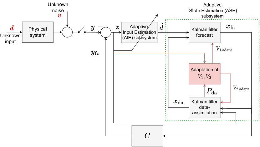
Figure 3: Block diagram of AISE.

IV-B Extremum-Seeking Control with Adaptive Input and State Estimation

For all $k\geq 1,$ let $y_{{\rm h},k}$ be updated by

$$y_{{\rm h},k}=f_{{\rm aise},k}(y_{{\rm g},k}).$$ (54)

Then, for all $k\geq 1,$ the update equations for ESC/AISE are given by (5), (6), (7), (54). Note that (54) replaces (4). The block diagram for ESC/AISE is shown in Figure 4.

Figure 4: Discrete-time extremum-seeking control with adaptive input and state estimation (ESC/AISE).

V Numerical Examples

In this section, we simulate ESC/AISE presented in Section IV to demonstrate its performance and compare it with discrete-time ESC outlined in Section III. To assess the accuracy of ESC/AISE, we define the root-mean-square error (RMSE) as

$${\rm RMSE}\stackrel{{\scriptstyle\triangle}}{{=}}\textstyle\sqrt{\frac{1}{k_{\rm end}-k_{\rm init}}\sum_{k=k_{\rm init}}^{k_{\rm end}}(u_{k}-u_{\rm opt})^{2}},$$ (55)

where $[k_{\rm init},k_{\rm end}]$ is the interval within which RMSE is computed, and $u_{\rm opt}$ represents the optimal input that either minimizes or maximizes the measured output. Note that $k_{\rm init}$ excludes the transient response and thus considers only the steady-state response. In Example V.1, the objective is to minimize a quadratic function with sensor noise, which extends Example 1 of [21] to include sensor noise. In Example V.2, the objective is to maximize the friction force applied by an antilock braking system (ABS) to a wheel with sensor noise, which extends [1, ch. 7] to include sensor noise.

Example V.1

Quadratic Cost. Consider

$$y(t)=\tfrac{1}{4}u^{2}(t),$$ (56)

where $u\in{\mathbb{R}}$ and $y\geq 0$. The objective is to minimize $y$ by modulating $u$ in the presence of sensor noise $v,$ such that, for all $k\geq 0,$

$$v_{k}=\begin{cases}0.5\sigma_{k},&k\in[0,1500],\\ \sigma_{k},&\mbox{otherwise},\end{cases}$$ (57)

where $\sigma_{k}\in{\mathbb{R}}$ is a Gaussian random variable with mean 0 and standard deviation $1;$ the sensor noise $v$ is shown in Figure 5. For all simulations in this example, the initial conditions are given by $u(0)=10$ and $y(0)=25.$ Since the system is a static map, the sampling rate is chosen to be $T_{\rm s}=1$ s without loss of generality and the results are presented in terms of steps.

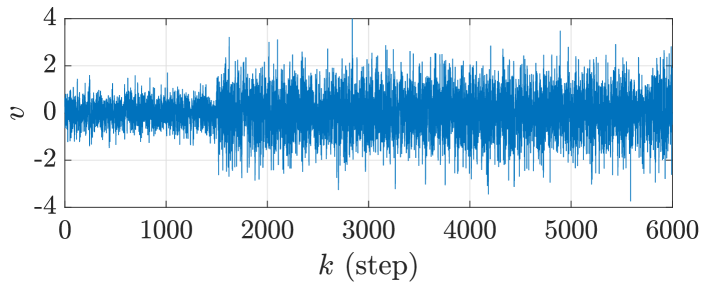
Figure 5: Example V.1: Quadratic Cost. Sensor noise $v$ defined in (57) added to $y$ for $k\in[0,6000]$.

The parameters for ESC are given by $K_{\rm g}=1$, $K_{\rm esc}=-1.5$, $K_{{\rm en},k}=1$, $\omega_{\rm esc}=\pi/4$ rad/step/s, $A_{\rm esc}=0.2$, $\omega_{\rm l}=2\pi/1000$ rad/step/s, $\omega_{\rm h}=2\pi/100$ rad/step/s, and $u_{0}=u(0)=10$. For ESC/AISE, the parameters are identical to those of ESC, with the exception of $\omega_{\rm h},$ which is not used. Additionally, the parameters for AISE are given by $n_{\rm e}=1$, $n_{\rm f}=2$, $R_{z}=1$, $R_{d}=10^{-8}$, $R_{\theta}=10^{-7}I_{3}$, $\eta=0.02$, $\tau_{n}=5$, $\tau_{d}=25$, $\alpha=0.02$, and $R_{\infty}=10^{4}$. The parameters $V_{1,k}$ and $V_{2,k}$ are adaptively updated with $\eta_{{\rm L}}=10^{-6}$, $\eta_{{\rm U}}=1$, and $\beta=0.5$, as described in Section IV-A3. For RMSE calculation, we set $k_{\rm init}=2000,$ $k_{\rm end}=6000,$ and $u_{{\rm opt},k}=0$ since this value minimizes $y.$

Figures 6 and 7 show the results of implementing ESC and ESC/AISE on the quadratic cost given by (56) with the sensor noise $v$ shown in Figure 5, which shows that, while both methods drive $u$ to a neighborhood of the minimizer 0, for all $k\geq 1500,$ the disruptions of $u$ due to sensor noise are less visible in the response of ESC/AISE, which shows that the performance of ESC/AISE is less degraded by sensor noise. To further test the sensitivity of ESC and ESC/AISE to sensor noise, 200 random trials are performed. The average RMSE values computed over the 200 trials are shown in Table I, which shows that, in the presence of sensor noise, ESC/AISE has overall better performance. $\diamond$

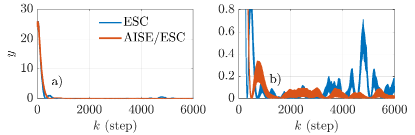
Figure 6: Example V.1: Quadratic Cost. System output $y$ for the quadratic cost given by (56) using ESC and ESC/AISE with the sensor noise $v$ shown in Figure 5. b) shows a) for all $y\in[0,0.8].$

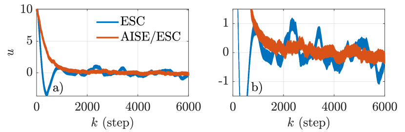
Figure 7: Example V.1: Quadratic Cost. Control input $u$ for the quadratic cost given by (56) using ESC and ESC/AISE with the sensor noise $v$ shown in Figure 5. b) shows a) for all $u\in[-1.5,1.5].$

TABLE I: Example V.1: Quadratic Cost. Average RMSE for ESC and ESC/AISE from 200 Monte Carlo trials.

Method	ESC	ESC/AISE
Average RMSE	$0.476$	$0.240$

Example V.2

Antilock Braking System (ABS). Consider an ABS implemented in a single-wheel system with dynamics

$$\dot{\nu} =-g\mu_{\lambda},$$ (58)

$$\dot{\Omega} =-\frac{B_{\rm f}}{J_{\rm w}}\Omega+\frac{mgR}{J_{\rm w}}\mu_{\lambda}-\tau_{\rm B},$$ (59)

where $\nu\in{\mathbb{R}}$ is the forward velocity of the center of the wheel, $\Omega\in{\mathbb{R}}$ is the angular velocity of the wheel, $m,R,J_{\rm w}$ are the mass, radius, and moment of inertia of the wheel, respectively, $B_{\rm f}$ is the bearing friction torque coefficient, $g$ is the acceleration due to gravity, $\tau_{\rm B}$ is the breaking torque, $\lambda>0$ is the wheel slip defined as

$$\lambda\stackrel{{\scriptstyle\triangle}}{{=}}\frac{\nu-R\Omega}{v},$$

where $\dot{\nu}<0$ and $R\Omega\leq\nu,$ and $\mu_{\lambda}$ is the friction force coefficient for all $\lambda>0.$ For simulation, $\mu_{\lambda}$ is defined as

$$\mu_{\lambda}\stackrel{{\scriptstyle\triangle}}{{=}}2\mu^{\star}\frac{\lambda^{\star}\lambda}{(\lambda^{\star})^{2}+\lambda^{2}},$$ (60)

where $\mu^{\star}$ is the maximum value of $\mu_{\lambda}$ and $\lambda^{\star}$ is the maximizer of $\mu_{\lambda},$ such that $\mu_{\lambda^{\star}}=\mu^{\star},$ as shown in Figure 8.

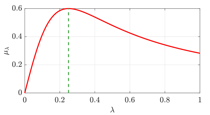
Figure 8: Example V.2: Antilock Breaking System. $\mu_{\lambda}$ versus $\lambda$ given by (60) for $\lambda^{\star}=0.25$ and $\mu^{\star}=0.6.$ The vertical, dashed green line indicates the value at which $\lambda=\lambda^{\star},$ which crosses the $\mu_{\lambda}$ versus $\lambda$ trace at $\mu_{\lambda^{\star}}=\mu^{\star},$ which is its maximum value.

We assume that $\dot{\nu}$ is measured by an accelerometer and $\tau_{\rm B}$ given by the feedback linearizing controller

$$\tau_{\rm B}=-\frac{cJ_{\rm w}\nu}{R}(\lambda-\lambda_{\rm d})-B_{\rm f}\Omega-\frac{J_{\rm w}\Omega}{\nu}\dot{\nu}-mR\dot{\nu},$$ (61)

where $c>0$ and $\lambda_{\rm d}>0$ is the designated value of $\lambda.$ Note that, when $\lambda_{\rm d}$ is constant, (61) and [1, p. 94, (7.4)] imply that, for all $t\geq 0,$ $\tilde{\lambda}(t)=\tilde{\lambda}(0)e^{-ct},$ where $\tilde{\lambda}\stackrel{{\scriptstyle\triangle}}{{=}}\lambda-\lambda_{\rm d}.$

The closed-loop system consisting of the single-wheel system with the ABS and the feedback linearizing controller is given by (58)–(61). The objective of the ABS is to maximize the stopping rate of the wheel, which is accomplished by reaching a value of $\lambda$ that maximizes $\mu_{\lambda},$ as shown by (58). Since the controller given by (61) modulates $\lambda_{\rm d}$ to reach a designated value of $\lambda,$ the objective is to determine $\lambda_{\rm d}$ such that $\mu_{\lambda}$ is maximized. Hence, the objective is to maximize $y\stackrel{{\scriptstyle\triangle}}{{=}}\mu_{\lambda}$ by modulating $u\stackrel{{\scriptstyle\triangle}}{{=}}\lambda_{\rm d}$ in the presence of sensor noise $v$ such that, for all $k\geq 0,$

$$v_{k}=\begin{cases}0.375\ \sigma_{k},&k\in[0,1250],\\ 0.75\ \sigma_{k},&\mbox{otherwise},\end{cases}$$ (62)

where $\sigma_{k}$ is a Gaussian random variable with mean 0 and standard deviation $1;$ the sensor noise $v$ is shown in Figure 9. Furthermore, for all simulations in this example, the wheel and feedback linearizing controller parameters are given by $m=400$ kg, $J_{\rm w}=1$ kg $\cdot$ m${}^{2},$ $R=0.3$ m, $B_{\rm f}=0.01$ kg $\cdot$ m²/s, $\lambda^{\star}=0.25,$ $\mu^{\star}=0.6,$ and $c=2,$ the initial conditions are given by $\lambda_{\rm d}(0)=0.1,$ $\nu(0)=336/3.6$ m/s and $\Omega(0)=1120/3.6$ rad/s, such that $\lambda(0)=0,$ and the sampling rate is given by $T_{\rm s}=0.01$ s. The continuous-time dynamics are simulated in Matlab by using ode45 with simulation time step 0.01 s. The simulation finalizes when the wheel stops, that is, $\nu$ reaches 0, or a maximum time limit of 50 s is reached. The time-to-stop $t_{\rm stop}>0$, which is defined by

$$t_{\rm stop}\stackrel{{\scriptstyle\triangle}}{{=}}\min\{t>0\colon\nu(t)=0\},$$

is used as the performance variable since the underlying objective of this problem is to stop the wheel as quickly as possible.

The parameters for ESC are given by $K_{\rm g}=1$, $K_{\rm esc}=1500$, $K_{{\rm en},k}=1$, $\omega_{\rm esc}=10$ rad/step/s, $A_{\rm esc}=0.01$, $\omega_{\rm l}=8$ rad/step/s, $\omega_{\rm h}=6$ rad/step/s, and $u_{0}=\lambda_{\rm d}(0)=0.1.$ For ESC/AISE, the parameters are identical to those of ESC, with the exception that the $\omega_{\rm h}$ parameter is no longer used. Additionally, for AISE are given by $n_{\rm e}=10$, $n_{\rm f}=20$, $R_{z}=1$, $R_{d}=10^{1}$, $R_{\theta}=10^{-2}I_{3}$, $\eta=0.001$, $\tau_{n}=2$, $\tau_{d}=10$, $\alpha=0.02$, and $R_{\infty}=10^{4}$. The parameters $V_{1,k}$ and $V_{2,k}$ are adaptively updated with $\eta_{{\rm L}}=10^{-8}$, $\eta_{{\rm U}}=10^{4}$, and $\beta=0.55$, as described in Section IV-A3. For RMSE calculation, we set $k_{\rm init}=5/T_{\rm s},$ $k_{\rm end}=\lfloor\min\{t_{\rm stop},50\}/T_{\rm s}\rfloor,$ and $u_{\rm opt}=\lambda^{\star}$ due to the maximum time limit of 50 s.

Figures 10 and 11 and Table II show the results of implementing ESC and ESC/AISE on the ABS dynamics given by (58)–(61) under no sensor noise, such that $v\equiv 0.$ These results show that ESC and ESC/AISE have similar maximization performance when no sensor noise is added to the ABS system measured output. Next, Figures 12 and 13 show the results of implementing ESC and ESC/AISE on the ABS dynamics given by (58)–(61) with the sensor noise $v$ shown in Figure 9. These results show that, while both methods stop the wheel and drive $\nu$ to 0, the disruptions due to the added sensor noise are less visible in the response of ESC/AISE, which also yields a lower value of $t_{\rm stop},$ which shows that the performance of ESC/AISE is less degraded by sensor noise. To further test the sensitivity of ESC and ESC/AISE to sensor noise, 100 random trials are performed. The average RMSE and average $t_{\rm stop}$ values computed over the 100 trials for the cases where ESC and ESC/AISE are implemented are shown in Table I. A stopping performance metric is also included in Table I, which shows the percentage of runs in which $\nu$ is driven to 0 before the 50-s time limit. These results show that ESC/AISE has an overall better maximization performance and is able to stop the wheel more consistently within the time limit in the presence of sensor noise. $\diamond$

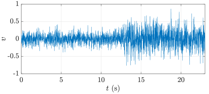
Figure 9: Example V.2: Antilock Breaking System. Sensor noise $v$ defined in (62) added to $y$ for $t\in[0,23]$ s.

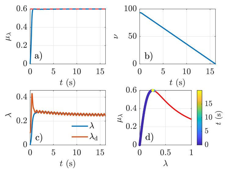
Figure 10: Example V.2: Antilock Breaking System. Results of implementing discrete-time ESC on the ABS dynamics given by (58)–(61) under no sensor noise, such that $v\equiv 0.$ a) shows $\mu_{\lambda}$ versus time, where the horizontal, dashed red line indicates the optimal value of $\mu$ given by $\mu^{\star}.$ b) shows $\nu$ versus time. c) shows $\lambda$ versus time and $\lambda_{\rm d}$ versus time. d) shows $\mu_{\lambda}$ versus $\lambda$ over time, where the red curve corresponds to $\mu_{\lambda}$ versus $\lambda$ given by (60) and shown in Figure 8.

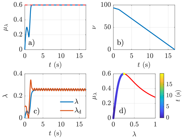
Figure 11: Example V.2: Antilock Breaking System. Results of implementing ESC/AISE on the ABS dynamics given by (58)–(61) under no sensor noise, such that $v\equiv 0.$ a) shows $\mu_{\lambda}$ versus time, where the horizontal, dashed red line indicates the optimal value of $\mu$ given by $\mu^{\star}.$ b) shows $\nu$ versus time. c) shows $\lambda$ versus time and $\lambda_{\rm d}$ versus time. d) shows $\mu_{\lambda}$ versus $\lambda$ over time, where the red curve corresponds to $\mu_{\lambda}$ versus $\lambda$ given by (60) and shown in Figure 8.

TABLE II: Example V.2: Antilock Breaking System. RMSE and $t_{\rm stop}$ for application of ESC and ESC/AISE on the ABS system without sensor noise.

Metric	ESC	ESC/AISE
RMSE	0.0080201	0.0074521
$\bm{t_{\rm stop}}$ (s)	16.41	16.81

Figure 12: Example V.2: Antilock Breaking System. Results of implementing discrete-time ESC on the ABS dynamics given by (58)–(61) with the sensor noise $v$ shown in Figure 9. a) shows $\mu_{\lambda}$ versus time, where the horizontal, dashed red line indicates the optimal value of $\mu$ given by $\mu^{\star}.$ b) shows $\nu$ versus time. c) shows $\lambda$ versus time and $\lambda_{\rm d}$ versus time. d) shows $\mu_{\lambda}$ versus $\lambda$ over time, where the red curve corresponds to the $\mu_{\lambda}$ versus $\lambda$ given by (60) and shown in Figure 8.

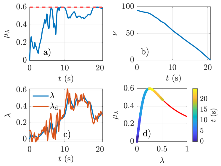
Figure 13: Example V.2: Antilock Breaking System. Results of implementing ESC/AISE on the ABS dynamics given by (58)–(61) with the sensor noise $v$ shown in Figure 9. a) shows $\mu_{\lambda}$ versus time, where the horizontal, dashed red line indicates the optimal value of $\mu$ given by $\mu^{\star}.$ b) shows $\nu$ versus time. c) shows $\lambda$ versus time and $\lambda_{\rm d}$ versus time. d) shows $\mu_{\lambda}$ versus $\lambda$ over time, where the red curve corresponds to $\mu_{\lambda}$ versus $\lambda$ given by (60) and Figure 8.

TABLE III: Example V.2: Antilock Breaking System. Average RMSE, average $t_{\rm stop},$ and stopping performance for application of ESC and ESC/AISE on an ABS system with sensor noise from 100 random trials.

Metric	ESC	ESC/AISE
Average RMSE	2.0281	0.22208
Average $\bm{t_{\rm stop}}$ (s)	30.3806	24.3548
$\begin{array}[]{l}\mbox{\bf Stopping}\\ \mbox{\bf performance}\end{array}$	Stopped 64% of the trials within 50 s	Stopped 100% of the trials within 50 s

VI Conclusions

This paper presented extremum-seeking control with adaptive input and state estimation (ESC/AISE) to improve optimization performance under sensor noise. ESC/AISE is obtained by replacing the high-pass filter in discrete-time ESC with AISE, which performs numerical differentiation in the presence of sensor noise. Numerical examples illustrate the performance of ESC/AISE and provide a comparison with ESC. These examples show that ESC/AISE offers better optimization performance than ESC in the presence of sensor noise. Future work will extend ESC/AISE to MIMO systems and variations of ESC, such as Newton-based ESC [13].

References

- [1] K. B. Ariyur and M. Krstić, Real-Time Optimization by Extremum-Seeking Control. John Wiley & Sons, 2003.
- [2] A. Scheinker, “100 years of extremum seeking: A survey,” Automatica, vol. 161, p. 111481, 2024.
- [3] A. S. Matveev, M. C. Hoy, and A. V. Savkin, “Extremum seeking navigation without derivative estimation of a mobile robot in a dynamic environmental field,” IEEE Trans. Contr. Syst. Tech., vol. 24, no. 3, pp. 1084–1091, 2015.
- [4] M. Bagheri, M. Krstić, and P. Naseradinmousavi, “Multivariable extremum seeking for joint-space trajectory optimization of a high-degrees-of-freedom robot,” J. Dyn. Syst. Meas. Contr., vol. 140, no. 11, p. 111017, 2018.
- [5] A. Ghaffari, M. Krstić, and S. Seshagiri, “Power optimization and control in wind energy conversion systems using extremum seeking,” IEEE Trans. Contr. Syst. Tech., vol. 22, no. 5, pp. 1684–1695, 2014.
- [6] D. Zhou, A. Al-Durra, I. Matraji, A. Ravey, and F. Gao, “Online energy management strategy of fuel cell hybrid electric vehicles: A fractional-order extremum seeking method,” IEEE Trans. Indust. Electr., vol. 65, no. 8, pp. 6787–6799, 2018.
- [7] A. Banaszuk, M. Ariyur, K. B .and Krstić, and C. A. Jacobson, “An adaptive algorithm for control of combustion instability,” Automatica, vol. 40, no. 11, pp. 1965–1972, 2004.
- [8] W. Liu, X. Huo, K. Ma, and W. Sun, “Improved gradient estimation for fast extremum seeking: A parametric proportional-integral observer-based approach,” IEEE Trans. Syst. Man Cybernetics: Syst., 2023.
- [9] M. Lanctot, K. Olofsson, M. Capella, D. Humphreys, N. Eidietis, J. Hanson, C. Paz-Soldan, E. Strait, and M. Walker, “Error field optimization in DIII-D using extremum seeking control,” Nuclear Fusion, vol. 56, no. 7, p. 076003, 2016.
- [10] S. Dubbioso, A. Jalalvand, J. Wai, G. De Tommasi, and E. Kolemen, “Model-free stabilization via extremum seeking using a cost neural estimator,” Expert Syst. Appl., p. 125204, 2024.
- [11] M. Krstić, “Performance improvement and limitations in extremum seeking control,” Sys. Contr. Lett., vol. 39, no. 5, pp. 313–326, 2000.
- [12] S.-J. Liu and M. Krstic, “Stochastic averaging in continuous time and its applications to extremum seeking,” IEEE Tran. Automat. Contr., vol. 55, no. 10, pp. 2235–2250, 2010.
- [13] A. Ghaffari, M. Krstić, and D. Nešić, “Multivariable newton-based extremum seeking,” Automatica, vol. 48, no. 8, pp. 1759–1767, 2012.
- [14] G. Gelbert, J. P. Moeck, C. O. Paschereit, and R. King, “Advanced algorithms for gradient estimation in one-and two-parameter extremum seeking controllers,” J. Proc. Contr., vol. 22, no. 4, pp. 700–709, 2012.
- [15] A. Scheinker and D. Scheinker, “Bounded extremum seeking with discontinuous dithers,” Automatica, vol. 69, pp. 250–257, 2016.
- [16] A. Mele, G. De Tommasi, and A. Pironti, “Finite-time stabilization of linear systems with unknown control direction via extremum seeking,” IEEE Trans. Automat. Contr., vol. 67, no. 10, pp. 5594–5601, 2021.
- [17] M. Guay and M. Benosman, “Finite-time extremum seeking control for a class of unknown static maps,” Int. J. Adap. Contr. Sig. Proc., vol. 35, no. 7, pp. 1188–1201, 2021.
- [18] A. Williams, A. Scheinker, E.-C. Huang, C. Taylor, and M. Krstic, “Experimental safe extremum seeking for accelerators,” IEEE Trans. Contr. Syst. Tech., 2024.
- [19] J. A. Paredes, R. Ramesh, M. Gamba, and D. S. Bernstein, “Experimental application of a quasi-static adaptive controller to a dual independent swirl combustor,” Combustion Science and Technology, pp. 1–34, 2024, dOI: 10.1080/00102202.2024.2306301.
- [20] J. A. Paredes, J. M. P. Delgado, D. S. Bernstein, and A. Goel, “Retrospective cost-based extremum seeking control with vanishing perturbation for online output minimization,” in Proc. Amer. Contr. Conf. IEEE, 2024, pp. 2344–2349.
- [21] M. S. Stanković and D. M. Stipanović, “Extremum seeking under stochastic noise and applications to mobile sensors,” Automatica, vol. 46, no. 8, pp. 1243–1251, 2010.
- [22] L. Brinón-Arranz and L. Schenato, “Consensus-based source-seeking with a circular formation of agents,” in Proc. Europ. Contr. Conf. IEEE, 2013, pp. 2831–2836.
- [23] N. A. Atanasov, J. Le Ny, and G. J. Pappas, “Distributed algorithms for stochastic source seeking with mobile robot networks,” J. Dyn. Syst. Meas. Contr., vol. 137, no. 3, p. 031004, 2015.
- [24] W. Wu and F. Zhang, “A speeding-up and slowing-down strategy for distributed source seeking with robustness analysis,” IEEE Trans. Contr. Network Sys., vol. 3, no. 3, pp. 231–240, 2015.
- [25] S.-J. Liu and M. Krstic, “Stochastic averaging in discrete time and its applications to extremum seeking,” IEEE Trans. Autom. Contr., vol. 61, no. 1, pp. 90–102, 2016.
- [26] M. S. Radenković, M. S. Stanković, and S. S. Stanković, “Extremum seeking control with two-sided stochastic perturbations,” SIAM J. Contr. Optim., vol. 56, no. 5, pp. 3766–3783, 2018.
- [27] A. Scheinker and D. Scheinker, “Extremum seeking for optimal control problems with unknown time-varying systems and unknown objective functions,” Int. J. Adaptive Contr. Sig. Proc., vol. 35, no. 7, pp. 1143–1161, 2021.
- [28] S. Sadatieh, M. Dehghani, M. Mohammadi, and R. Boostani, “Extremum-seeking control of left ventricular assist device to maximize the cardiac output and prevent suction,” Chaos, Solitons & Fractals, vol. 148, p. 111013, 2021.
- [29] B. Zhao, X. Yang, and E. Fridman, “A time-delay approach to extremum seeking with measurement noise,” IFAC-PapersOnLine, vol. 56, no. 2, pp. 2413–2418, 2023.
- [30] X. Yang, B. Zhao, and E. Fridman, “A time-delay approach to multi-variable extremum seeking with measurement noise,” in Proc. Eur. Contr. Conf., 2024, pp. 531–536.
- [31] L. Dewasme and A. V. Wouwer, “Stabilizing extremum seeking control applied to model-free bioprocess productivity optimization,” IFAC-PapersOnLine, vol. 58, no. 14, pp. 712–717, 2024.
- [32] S. Verma, S. Sanjeevini, E. D. Sumer, and D. S. Bernstein, “Real-time Numerical Differentiation of Sampled Data Using Adaptive Input and State Estimation,” International Journal of Control, pp. 1–13, 2024.
- [33] S. Verma, B. Lai, and D. S. Bernstein, “Adaptive Real-Time Numerical Differentiation with Variable-Rate Forgetting and Exponential Resetting,” in Proc. Amer. Contr. Conf., 2024, pp. 3103–3108.
- [34] S. Verma, S. Sanjeevini, E. D. Sumer, A. Girard, and D. S. Bernstein, “On the Accuracy of Numerical Differentiation Using High-Gain Observers and Adaptive Input Estimation,” in Proc. Amer. Contr. Conf., 2022, pp. 4068–4073.
- [35] S. A. U. Islam and D. S. Bernstein, “Recursive least squares for real-time implementation,” IEEE Contr. Syst. Mag., vol. 39, no. 3, pp. 82–85, 2019.
- [36] B. Lai and D. S. Bernstein, “Exponential Resetting and Cyclic Resetting Recursive Least Squares,” IEEE Contr. Sys. Lett., vol. 7, pp. 985–990, 2022.
- [37] K. J. Åström, U. Borisson et al., “Theory and Applications of Self-Tuning Regulators,” Automatica, vol. 13, no. 5, pp. 457–476, 1977.
- [38] O. Malik, G. Hope, and S. Cheng, “Some Issues on the Practical Use of Recursive Least Squares Identification in Self-Tuning Control,” Int. J. Contr., vol. 53, no. 5, pp. 1021–1033, 1991.
- [39] N. Mohseni and D. S. Bernstein, “Recursive least squares with variable-rate forgetting based on the F-test,” in Proc. Amer. Contr. Conf., 2022, pp. 3937–3942.