Quantum Machine Learning of Molecular Energies with Hybrid Quantum-Neural Wavefunction

Abstract

Quantum computational chemistry holds great promise for simulating molecular systems more efficiently than classical methods by leveraging quantum bits to represent molecular wavefunctions. However, current implementations face significant limitations in accuracy due to hardware noise and algorithmic constraints. To overcome these challenges, we introduce a hybrid framework that learns molecular wavefunction using a combination of an efficient quantum circuit and a deep neural network. This approach enhances computational efficiency and accuracy, surpassing traditional quantum computational chemistry methods. Numerical benchmarking on molecular systems shows that our hybrid quantum-neural wavefunction approach achieves near-chemical accuracy, comparable to advanced quantum and classical techniques. Experimental validation on a superconducting quantum computer, using the isomerization reaction of cyclobutadiene, further demonstrates its practical applicability, with high accuracy in energy estimation and significant resilience to noise.

I Introduction

Quantum computers leverage quantum effects to store and manipulate data, making them particularly suitable for the simulation of microscopic quantum systems [1, 2, 3, 4]. However, the implementation of useful algorithms on current quantum hardware faces serious challenges due to significant gate noise and limited coherence time [5, 6, 7]. Despite ongoing efforts to develop fault-tolerant quantum computers [8, 9, 10, 11, 12], the Variational Quantum Eigensolver (VQE) algorithm remains the most widely adopted framework for quantum computational chemistry [13, 14, 15]. The key component of the VQE algorithm is the parameterized quantum circuit, a variational form for the quantum state of the system under study, also known as an ansatz in classical computational chemistry. The VQE approach can be considered a quantum version of deep learning, where the parameters in the circuit are trained to minimize an energy loss function [16]. Through a decade of development, two main families of ansatz have been established for quantum computational chemistry: the Unitary Coupled-Cluster (UCC) ansatz [17] and the Hardware-Efficient Ansatz (HEA) [18]. UCC offers high accuracy but its implementation on current hardware is challenging due to the deep circuit depths required [19, 20, 21]. HEA is designed for hardware compatibility, which makes it a popular choice for demonstrations of recent quantum hardware [22, 23, 24, 25]. However, HEA often struggles with accuracy and scalability [26, 27]. The paired UCC with Double excitations (pUCCD) circuit has recently gained attention as a hardware-efficient variant of UCC circuits [28, 29]. pUCCD uses $N$ qubits to represent $N$ molecular spatial orbitals by enforcing electron pairing, a significant improvement over the typical $2N$ qubit requirement. Futhermore, the pUCCD circuit can be compiled into an efficient circuit with a depth of $N$. These advantages have led to the successful application of pUCCD in the quantum computation of molecular energies on both superconducting and trapped-ion quantum computing platforms [30, 31, 32]. However, pUCCD’s neglect of configurations with single orbital occupations leads to errors exceeding 100 mHartree for simple molecules such as Li2O, which are far above the chemical accuracy threshold of 1.6 mHartree. While efforts have been made to enhance the accuracy through orbital optimization (oo-pUCCD) [33, 34, 31], a significant gap remains in accurately describing singly occupied configurations [35, 36].

Parallel to the evolution of VQE, Deep Neural Networks (DNNs) have shown remarkable success in representing quantum wavefunctions of chemical systems [37]. Based on variational Monte Carlo, these DNNs are trained to minimize the energy expectation. Efforts along this line include DeepWF [38], FermiNet [39], PauliNet [40], QiankunNet [41], and so on [42, 43, 44, 45]. Thanks to the expressive power of DNNs, these methods demonstrate accuracy comparable to Coupled Cluster with Single and Double excitations (CCSD) but with significantly lower computational scaling, typically $\mathcal{O}(N^{4})$. This success has inspired the development of hybrid quantum-neural wavefunctions, where quantum circuits and neural networks are jointly trained to represent the wavefunction of quantum systems [46]. In this hybrid approach, quantum circuits are responsible for learning the quantum phase structure of the target state, which is a difficult task for neural networks alone. The intersection between quantum computing and machine learning, known as quantum machine learning, is developing at a rapid pace [47, 48, 49, 50]. Chemistry applications include the construction of shallow depth ansatz, energy eigenstate filtration, material phase prediction, neural network pertaining, and so on [51, 52, 53, 54, 55, 56].

In this work, we propose a quantum machine learning framework for efficient representation of molecular wavefunction and accurate computation of molecular energies. The method employs the linear-depth pUCCD circuit to learn molecular wavefunction in the seniority-zero subspace, and a deep neural network to correctly account for the contributions from singly occupied configurations. The expansion of the quantum space is achieved by careful quantum circuit design, which enables an efficient algorithm for computing the expectations of physical observables for the hybrid quantum-neural wavefunction. As a result, our method, named pUCCD-DNN, retains the low qubit count ($N$ qubits) and shallow circuit depth of pUCCD, while achieving accuracy comparable to the most precise quantum and classical computational chemistry methods, such as UCCSD (UCC with single and double excitations) and CCSD(T) (CCSD with perturbative triple excitations). We demonstrate the efficacy of pUCCD-DNN through numerical simulations of various diatomic and polyatomic molecular systems, such as N2 and CH4. To test pUCCD-DNN in a real quantum computing scenario, we compute the reaction barrier for the isomerization of cyclobutadiene on a programmable superconducting quantum computer. The results demonstrate that the pUCCD-DNN is highly accurate and noise resilientfor a real quantum computing task.

II Results

II.1 The pUCCD-DNN method

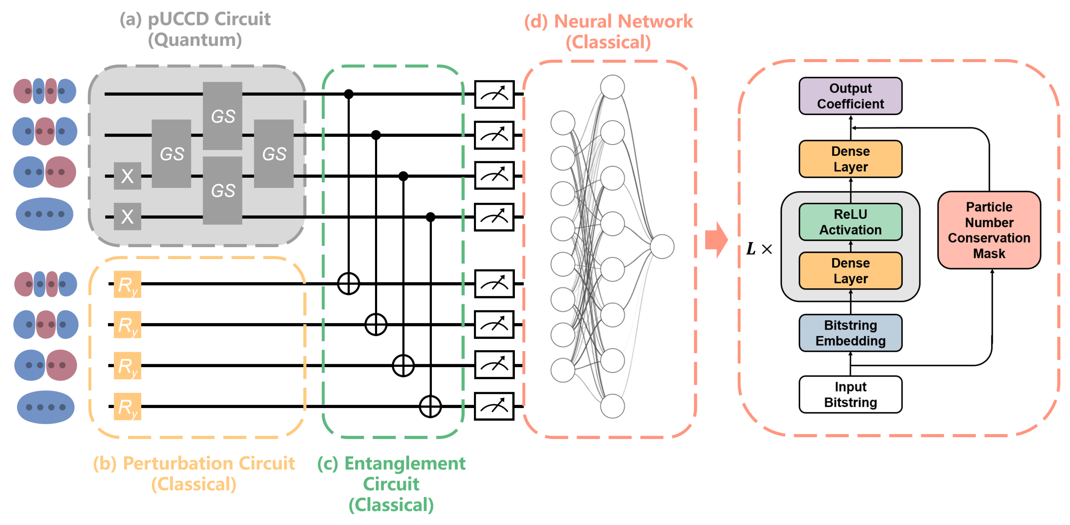
Figure 1: A Schematic diagram for the pUCCD-DNN framework. The pUCCD circuit in the grey box is the only component executed on a real quantum computer. “GS” denotes Givens-Swap gate. Meanwhile, the perturbation circuit and the entanglement circuit are processed classically. Together, the quantum circuit and the neural network serves as an ansatz and are trained jointly to represent the molecular wavefunction.

In this section, we present our pUCCD-DNN algorithm and focus on our contribution. General backgrounds, such as the electronic structure problem and the UCC types of ansatz for quantum computational chemistry are briefly overviewed in the Methods section.

We start by employing the pUCCD ansatz to represent molecular wavefunction, which is encoded in the parameterized quantum circuit $\hat{U}(\vec{\theta})$. pUCCD uses one qubit to represent a pair of electrons, and thus reduces the number of qubits required for an $N$-orbital molecule from $2N$ to $N$. The pUCCD method neglects the contributions from singly-occupied configurations, and the pUCCD-DNN framework addresses this limitation by a series of ancilla quantum circuits and a deep neural network, with a manageable measurement overhead.

To correctly describe the singly occupied configurations, we add $N$ ancilla qubits to the circuit and expand the Hilbert space from $N$ qubits to $2N$ qubits. We note that these $N$ ancilla qubits can be treated classically, which will be explained later, and our pUCCD-DNN algorithm preserves the $N$-qubit quantum resource requirement instead of $2N$ in other methods. In the computational basis, the circuit state can be expressed as

$$\ket{\psi}=\sum_{k}a_{k}\ket{k}\ ,$$ (1)

where $\ket{k}$ represents the occupation of a pair of electrons in the original $N$-qubit Hilbert space. In the expanded $2N$-qubit space, the equivalent state is

$$\ket{\Phi}=\sum_{k}a_{k}\ket{k}\otimes\ket{k}\ ,$$ (2)

with the two $\ket{k}$ terms now representing the occupation of the alpha and beta spin sectors, respectively. For ground state problems, the coefficients $a_{k}$ can be assumed to be real numbers.

In the context of quantum circuits, the expanded state $\ket{\Phi}$ is constructed from $\ket{\psi}$ using the ancilla qubits and an entanglement circuit $\hat{E}$:

$$\ket{\Phi}=\hat{E}\left(\ket{\psi}\otimes\ket{0}\right)\ .$$ (3)

The entanglement circuit $\hat{E}$ creates the necessary correlations between the original qubits and the ancilla qubits. It can be decomposed into $N$ parallel CNOT gates:

$$\hat{E}=\prod_{i}^{N}\textrm{CNOT}_{i,i+N}\ ,$$ (4)

where each CNOT gate entangles the $i$-th original qubit with the corresponding $i$-th ancilla qubit.

Although $\ket{\Phi}$ has $2N$ qubits while $\ket{\psi}$ has $N$ qubits, from a quantum chemistry perspective, they represent the same state in the seniority-zero space and therefore have the same energy. To improve the representation, we propose to apply a non-unitary post-processing operator [46], $\hat{N}$, defined in the expanded Hilbert space. The method is known as variational quantum-neural hybrid eigensolver (VQNHE) and it provides exponential acceleration for nonunitary postprocessing in VQE than naive transformed Hamiltonian approach [57, 58, 59]. This operator $\hat{N}$ augments the state $\ket{\Phi}$ as follows:

$$\hat{N}=\sum_{kj}b_{kj}\ket{k}\ket{j}\bra{j}\bra{k}\ ,$$ (5)

where $b_{kj}$ is a real high dimensional tensor with $2^{2N}$ elements. At first glance, handling such a large tensor seems computationally intractable. To address the problem, we generalize $b_{kj}$ to a function and employ a deep neural network $\mathcal{B}(k,j)$ to represent $b_{kj}$, such that $b_{kj}=\mathcal{B}(k,j)$. After applying $\hat{N}$, the overall state becomes

$$\hat{N}\hat{E}\left(\ket{\psi}\otimes\ket{0}\right)=\sum_{k}a_{k}b_{kk}\ket{k}\otimes\ket{k}\ .$$ (6)

Although $\hat{N}$ modulates the coefficients $a_{k}$, $\hat{N}$ can not recover the missing single-occupied configurations, since their contribution in $\ket{\Phi}$ is strictly zero. To deal with this problem, we apply a perturbation circuit $\hat{P}$ to the ancilla qubits at the beginning, such that the state of the ancilla qubits $\ket{\phi}=\hat{P}\ket{0}$ deviates slightly from $\ket{0}$

$$\ket{\phi}=\hat{P}\ket{0}=\frac{\ket{0}+\sum_{j\neq 0}\epsilon_{j}\ket{j}}{1+\sum_{j\neq 0}\epsilon^{2}_{j}}\ ,$$ (7)

where $\epsilon_{j}$ are small coefficients satisfying $\sum_{j\neq 0}\epsilon_{j}^{2}\ll 1$. The updated $\ket{\Phi}$ primarily consists of states in the seniority-zero space. The states outside of the seniority-zero space are introduced with small coefficients $a_{k}\epsilon_{j}$ These contributions can later be refined through the variational principle and the deep neural network.

The values of $\epsilon_{j}$ and the exact form of $\hat{P}$ are flexible, since the role of $\hat{P}$ is to introduce the missing components and the overall wavefunction is optimized variationally. As a result, our algorithm is expected to be resilient to noise [60], making it well-suited for implementation on real quantum devices. The only key requirement for $\hat{P}$ is that it should have a low circuit depth, which allows efficient simulation of $\hat{P}\ket{0}$ on classical computers. In this work, we adopt a perturbation circuit with single qubit rotation gates $R_{y}$ for each qubit and the rotation angle is set to 0.2. The $R_{y}$ gates are chosen because they produce real coefficients, a desired property for the ground state of the molecular Hamiltonian.

After describing the quantum circuit part, we turn to the deep neural network structure used for $\mathcal{B}(k,j)$. In this work, we focus on a simple and interpretable neural network architecture. More extensive neural network architecture searches and incorporation of additional physical intuition are left for future research. $\mathcal{B}(k,j)$ accepts the two bitstring $k$ and $j$ as input and outputs the coefficients $b_{kj}$, which modulates the coefficients of the configuration $\ket{k}\ket{j}$ in the final molecular wavefunction. The first component of the neural network is embedding the bitstring $\ket{k}\otimes\ket{j}$ into a vector. We employ a straightforward binary representation, where $\ket{k}\otimes\ket{j}$ is converted to a vector of size $2N$, with each element being either -1 or 1. The vector $\mathbf{x}_{0}(k,j)$ is then passed through a deep neural network consisting of $L$ dense layers and ReLU activation functions

$$\mathbf{x}_{i+1}(k,j)=\textrm{ReLU}\left[\mathbf{W}_{i}\mathbf{x}_{i}(k,j)+\mathbf{c}_{i}\right]\ .$$ (8)

In the hidden layers, the number of neurons is set to $2KN$ where $K$ is a tunable integer that controls the size of the neural network. In this work, we set $K=2$ unless otherwise specified. The number of layers $L$ is chosen to be proportional to the size of the molecule. More specifically, we employ $L=N-3$ in this work. For example, with STO-3G basis set, H4, with $N=4$ orbitals, has 1 hidden layer, while H8, with $N=8$ orbitals, has 5 hidden layers. The number of parameters in the neural network scales as $K^{2}N^{3}$ considering both the width and depth of the neural network. The computational complexity is also $\mathcal{O}(K^{2}N^{3})$ for each input bitstring.

The final dense layer outputs the desired coefficient $b_{kj}$, before multiplying with the particle number conservation mask $m(k,j)$

$$b_{kj}=m(k,j)\left[\mathbf{W}_{L}\mathbf{x}_{L}(k,j)+\mathbf{c}_{L}\right]\ .$$ (9)

The mask $m(k,j)$ is defined as

$$m(k,j)=\begin{cases}\mathbf{1}&\textrm{if}\quad\sum_{i}k_{i}=N_{\alpha}\quad\textrm{and}\quad\sum_{i}j_{i}=N_{\beta},\\ \mathbf{0}&\textrm{otherwise}\end{cases}$$ (10)

where $N_{\alpha/\beta}$ are the number of spin up/down electrons. The purpose of this mask is to set $b_{kj}$ to 0 if the corresponding configuration $\ket{k}\otimes\ket{j}$ does not conserve the number of spin up and down electrons.

To summarize, the overall wavefunction is given by

$$\ket{\Psi}=\hat{N}\hat{E}\left(\hat{U}(\vec{\theta})\ket{0}\otimes\hat{P}\ket{0}\right)\ ,$$ (11)

which consists of four components: the pUCCD circuit $\hat{U}(\vec{\theta})$, the perturbation circuit $\hat{P}$, the entanglement circuit $\hat{E}$ and the neural network $\hat{N}$. The next challenge is to measure the expectation value of the energy based on Eq. (11). It is highly nontrivial to measure the energy expectation without resorting to quantum tomography or incurring exponential measurement overhead. Without an efficient measurement protocol, the pUCCD-DNN approach could be rendered impractical. In fact, the ansatz represented by Eq. (11) is carefully designed in such a way that an efficient algorithm for computing expectation values is possible. Since $\ket{\Psi}$ is not normalized, the energy expectation is

$$\braket{E}=\frac{\braket{\Psi|\hat{H}|\Psi}}{\braket{\Psi|\Psi}}\ .$$ (12)

The next step is to develop a measurement protocol that enables the computation of both $\braket{\Psi|\hat{H}|\Psi}$ and $\braket{\Psi|\Psi}$ using the measurement outcome of the quantum circuit $\hat{U}(\vec{\theta})\ket{0}$ and the output from the deep neural network.

Here we outline the key points of the measurement protocol and the full measurement protocol is provided in the Method section. For brevity, we assume there is only a single Pauli string in $\hat{H}$, and the summation over many Pauli strings can be handled straightforwardly. We also note that the estimation of the norm $\braket{\Psi|\Psi}$ can be considered as a special case when $\hat{H}=\hat{I}$.

To perform the measurement, we transform the Hamiltonian to be measured with $\hat{E}$ and $\hat{N}$

$$\braket{\Psi|\hat{H}|\Psi}=\braket{\psi\otimes\phi|\left(\hat{E}^{\dagger}\hat{N}^{\dagger}\hat{E}\right)\left(\hat{E}^{\dagger}\hat{H}\hat{E}\right)\left(\hat{E}^{\dagger}\hat{N}\hat{E}\right)|\psi\otimes\phi}\ .$$ (13)

Since $\hat{E}$ is a Clifford circuit, $\hat{H}^{\prime}=\hat{E}^{\dagger}\hat{H}\hat{E}$ is also a Pauli string.

Additionally, since $\hat{E}$ is composed of CNOT gates, it reversibly maps one bitstring to another, rather than a linear combination of bitstrings. Specifically,

$$\hat{E}\left(\ket{k}\otimes\ket{j}\right)=\ket{k}\otimes\ket{k\oplus j}\ .$$ (14)

The transformed neural network $\hat{N}^{\prime}=\hat{E}^{\dagger}\hat{N}\hat{E}$ is

$$\hat{N}^{\prime}=\sum_{kj}b_{kj}\ket{k}\ket{k\oplus j}\bra{k\oplus j}\bra{k}=\sum_{kj}b_{k,k\oplus j}\ket{k}\ket{j}\bra{j}\bra{k}\ .$$ (15)

$\hat{N}^{\prime}$ is thus formally the same as $\hat{N}$ but with a permuted index for the coefficient $b$.

The expression of the expectation in Eq. (13) becomes

$$\braket{\Psi|\hat{H}|\Psi}=\braket{\psi\otimes\phi|\hat{N}^{\prime\dagger}\hat{H}^{\prime}\hat{N}^{\prime}|\psi\otimes\phi}\ ,$$ (16)

which corresponds to the measurement of $\hat{N}^{\prime\dagger}\hat{H}^{\prime}\hat{N}^{\prime}$ on two unentangled circuit $\ket{\psi}$ and $\ket{\phi}$. If $\hat{N}^{\prime}$ is absent or if $\hat{N}^{\prime}=\hat{I}$, the measurement of $\hat{H}$ can be performed efficiently by measuring the two separate circuits $\ket{\psi}$ and $\ket{\phi}$. In the Methods section, we show that, by carefully designing the measurement circuit, $\hat{N}^{\prime}\hat{H}^{\prime}\hat{N}^{\prime}$ can also be measured by separate measurement of $\ket{\psi}$ and $\ket{\phi}$, with a constant overhead. Therefore, the evaluation of $\braket{\Psi|\hat{H}|\Psi}$ is cast into the separate measurement of $\ket{\psi}$ and $\ket{\phi}$. Since $\ket{\phi}$ is designed to be a shallow circuit that can be efficiently simulated classically, the only circuit that needs to be executed on real quantum devices is the pUCCD circuit $\ket{\psi}$.

Therefore, pUCCD-DNN uses $N$ qubits and $N$ circuit depth for molecular wavefunction learning. The contribution from seniority-zero space to the overall wavefunction is recovered through classical post-processing, without requiring additional quantum resources. Nonetheless, the number of terms to measure in the Hamiltonian increases from $N^{2}$ in the pUCCD circuit to $N^{4}$ for more general electronic structure problems.

A schematic diagram of the pUCCD-DNN framework is depicted in Fig. 1. In the whole algorithm, only the pUCCD circuit within the grey box in dashed lines is executed on quantum computers, which allows pUCCD-DNN to maintain the $N$-qubit requirement for the computation instead of $2N$. The perturbation circuit and entanglement circuit can be efficiently processed on classical computers. The measured bitstring of the composite circuit is fed into the neural network for $\mathcal{B}(k,j)$, which is then used to adjust the measurement outcome. The entire ansatz is then set up in a VQE workflow, where both the parameters in the quantum circuit and the neural network are trained to minimize the molecular energy. This process ultimately yields the ground state through the variational principle.

II.2 Accuracy and Scalability

We first compare the error of pUCCD-DNN with other quantum computational methods in Fig. 2. For this comparison, we perform noiseless numerical calculations on second-periodic small molecules ranging from 2 atoms to 5 atoms. The basis set employed is STO-3G and the $1s$ orbitals are frozen. Since there are 8 spatial orbitals, the systems correspond to 8 qubits for paired ansatz and 16 qubits otherwise. The exact geometries of the molecules are reported in the Supplementary Information. The full configuration interaction (FCI) energy for these molecules is computed as the reference energy.

The standard pUCCD approach improves over the HF method but consistently shows the highest error across all molecules. pUCCD is computationally efficient because it uses $N$ qubits for $N$ molecular orbitals. Yet the neglect of singly-occupied configurations limits its accuracy. The oo-pUCCD method reduces the error to a modest extent for most molecules, except for N2 and CO, where the errors of pUCCD and oo-pUCCD are comparable. This demonstrates the limitation of oo-pUCCD, as it still assumes electron paring and it also uses $N$ qubits for $N$ molecular orbitals. The UCCSD method, known for its high accuracy, performs well across the board. However, it requires $2N$ qubits for $N$ molecular orbitals and has a very deep circuit, which is computationally expensive. This highlights the significant error introduced by the assumption of electron pairing. In contrast, our proposed pUCCD-DNN method stands out as the most accurate approach for the majority of the molecules studied. pUCCD-DNN frequently achieves or approaches chemical accuracy, as indicated by the shaded area on the graph. The deep neural network attached to the quantum circuit effectively corrects for the non-pairing electron configurations, which significantly improves accuracy. An important feature of pUCCD-DNN is that it uses only $N$ qubits for $N$ molecular orbitals, and its circuit depth is the same as the circuit depth of pUCCD. The enlarged Hibert space is introduced by an ancilla circuit that can be simulated classically. By comparing pUCCD-DNN and pUCCD, we find that, the mean absolute error (MAE) decreases from 51.9 mHartree for pUCCD to 0.6 mHartree for pUCCD-DNN. This corresponds to a reduction in error by two orders of magnitude. The MAE of pUCCD-DNN is comparable to the MAE of UCCSD, which is 1.9 mHartree.

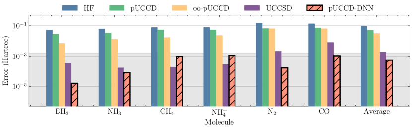
Figure 2: Compare the error of pUCCD-DNN with other quantum computational chemistry methods. The pUCCD-DNN energy is obtained by noiseless simulator and the reference energy is FCI. The shaded area indicates the chemical accuracy.

In Fig. 3 we compare the error of pUCCD-DNN with several classical computational methods. The doubly occupied configuration interaction (DOCI) method is the classical counterpart of the pUCCD method since it also assumes electron pairing. Based on the results in Fig. 2 we can expect DOCI will perform poorly, which is confirmed by the data in Fig. 3. The Møller–Plesset perturbation theory of second order (MP2) improves over DOCI, particularly for diatomic molecules. This suggests that including singly occupied configurations is crucial for accurately describing the molecular wavefunction. The coupled-cluster methods, CCSD and its perturbative extension CCSD(T), are considered some of the most accurate techniques in quantum chemistry. The accuracy of these methods is also shown in Fig. 3. Both CCSD and CCSD(T) demonstrate high accuracy, with CCSD(T) achieving chemical accuracy for most of the molecules studied. When comparing pUCCD-DNN to these classical methods, we find that pUCCD-DNN achieves accuracy comparable to that of CCSD(T), indicating that pUCCD-DNN is a high-accuracy method for quantum chemistry calculations.

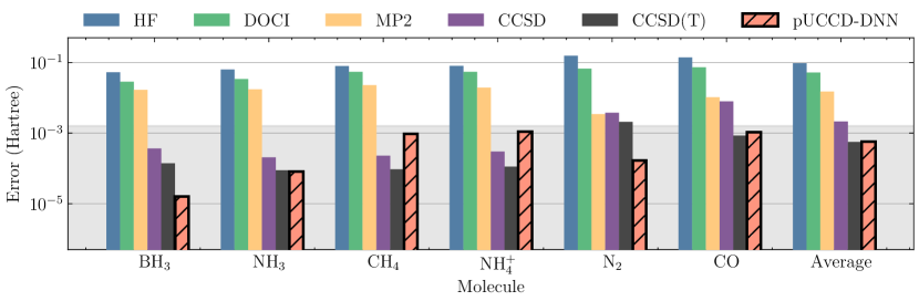
Figure 3: Compare the error of pUCCD-DNN with other classical computational chemistry methods. The pUCCD-DNN energy is obtained by noiseless simulator and the reference energy is FCI. The shaded area indicates the chemical accuracy.

We next investigate the factors that determine the accuracy of the pUCCD-DNN method. Fig. 4(a) compares the error of pUCCD and pUCCD-DNN methods against the size of hydrogen chain molecules (H5+, H6, H7+, and H8) for two different bond lengths ($d$ = 1.0 Å and $d$ = 2.5 Å). The results clearly demonstrate that pUCCD-DNN consistently outperforms standard pUCCD, achieving lower error across all molecule sizes and bond lengths. Notably, pUCCD-DNN maintains high accuracy even as the molecule size increases especially for the longer bond length of 2.5 Å. When $d=1.0Å$, the errors of pUCCD-DNN seem to fluctuate when the system size varies. However, the magnitude of the fluctuation, in the order of $10^{-4}$, is well below the chemical accuracy threshold and thus insignificant. Fig. 4(b) showcases the impact of neural network size on the error of pUCCD-DNN for various molecules. The $x$-axis represents the neural network size $K$, where the number of hidden neurons is $2KN$ ($N$ is the number of molecular orbitals). The atomic distance in H8 is $d$ = 1.0 Å. As the network size increases from 2 to 8, there’s a clear trend of a logarithmic decreasing error for all molecules. Most molecules achieve chemical accuracy (indicated by the shaded area) with larger neural networks, with NH3 and BH3 showing particularly significant improvements in accuracy as the network size grows. We note that the molecules studied here are still much smaller than those typically encountered in practical chemistry problems. Scaling up to larger systems will require emulating more complex quantum circuits and performing intensive classical computations, which will be the subject of our future work.

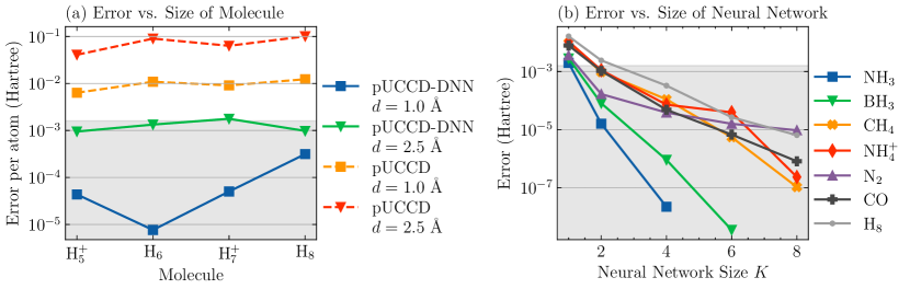
Figure 4: Factors for the accuracy of the pUCCD-DNN method based on noiseless simulation. (a) The error of pUCCD-DNN versus the size of the molecule under study. (b) The error of pUCCD-DNN versus the size of the neural network $k$. The number of hidden neurons in the deep neural network is $2kN$ where $N$ is the number of molecular orbitals. The shaded area indicates the chemical accuracy.

We finally test the accuracy of pUCCD-NN based on cubic H8 molecule at different H-H distance $d$. The system is particularly challenging due to the strong correlation as $d$ increases. In Fig. 5(a) we show the potential energy profile computed by both pUCCD-DNN and pUCCD. From $d=0.5$ Å to 2.5 Å pUCCD-DNN coincides well with the FCI solution. In contrast, the pUCCD method shows a considerable amount of error at intermediate $d$ ($d=1.0$ Å) and completely fails to describe the dissociation limit. For reference, we also include the CCSD method, which shows high accuracy at intermediate $d$. However, the error of CCSD quickly increases as $d$ becomes larger than 1.5 Å and it fails to reach convergence for larger $d$. CCSD(T) is not expected to improve CCSD when it fails because CCSD(T) relies on good CCSD wavefunction to account for perturbative triple excitation. In Fig. 5(b) we depicted the error of the methods in logarithmic scale. All methods except pUCCD-DNN show an increase in error as $d$ increases. The maximum error for pUCCD-DNN appears at $d=1.7$ Å. The UCCSD method is also included in Fig 5. While UCCSD also shows high accuracy at smaller $d$, it suffers from significant error at the large $d$ limit, similar to CCSD.

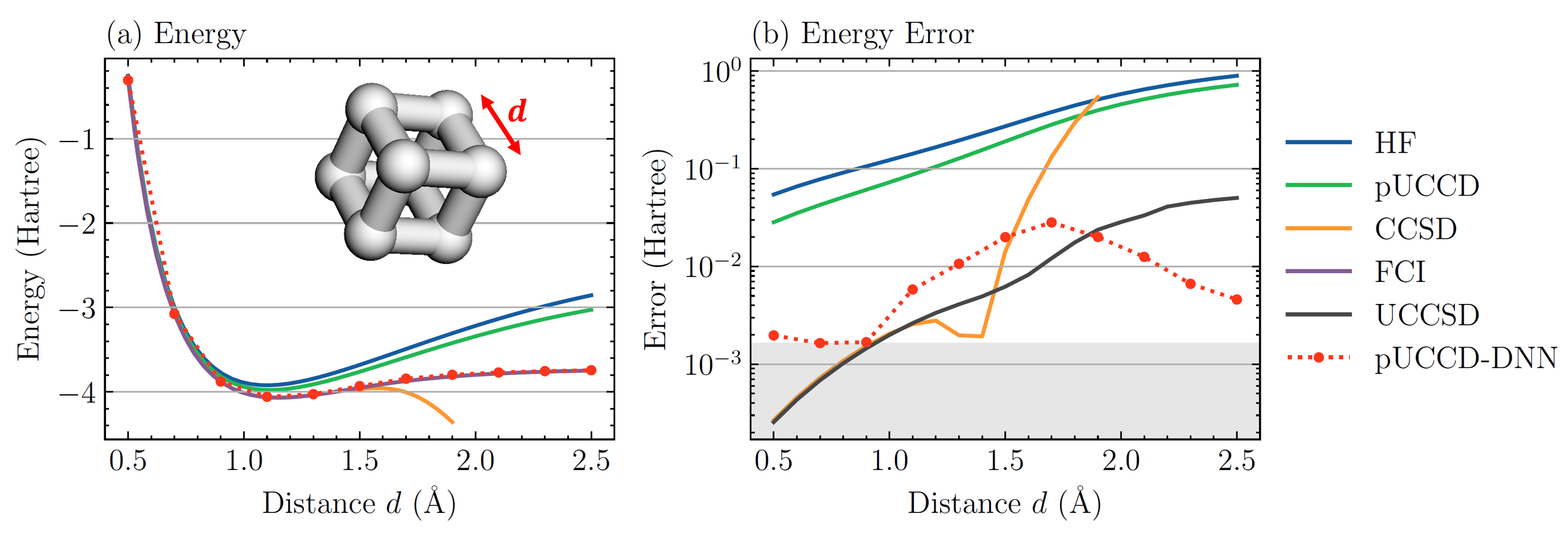
Figure 5: Benchmarking noiseless pUCCD-DNN based on the potential energy profile of cubic H8. (a) The potential energy profile of cubic H8 by different computational methods. (b) The error compared with the exact solution versus the H-H distance in the H8 cube.

II.3 Experiments on a Superconducting Quantum Computer

To evaluate the performance of pUCCD-DNN in a real quantum computing scenario, we conduct experiments on a superconducting quantum computer. We choose the isomerization reaction of cyclobutadiene as our model system, as shown in Fig. 6(a). The transition state of this system is particularly challenging due to strong correlations arising from degeneracy [61]. This system has previously been used to demonstrate the high accuracy of PauliNet [40]. In this reaction, the reactant and product are identical molecules, with a 90-degree rotation between them. The electronic structures of the reactant and the product are considerably simpler than that of the transition state. Therefore, in the following analysis, we focus on the transition state, and calculate the reaction barrier by subtracting the FCI energy of the reactant and product from the energy of the transition state.

We employ the cc-pVDZ basis set [62] for HF calculation. For the active space, we select four orbitals: HOMO-1, HOMO, LUMO, and LUMO+1. These correspond to the frontier molecular orbitals formed by the four C $2p_{z}$ orbitals. Using the paired ansatz, the active space is represented by a 4-qubit quantum circuit, with four parameters corresponding to four distinct excitations. The superconducting quantum chip used in this work consists of 13 qubits. Since the Givens-Swap gate is not a native gate on this chip, we carefully select 4 qubits from the 13-qubit system, which follows a ring topology (shown in Fig. 6(d)). This selection allows us to implement all four excitation operators using only Givens rotation gates, eliminating the need for the more expensive swap gates, which would otherwise require 3 CNOT gates. The Givens rotation gates should be further compiled into 4 native CNOT gates, along with several single-qubit gates. To reduce circuit depth, we introduce an approximation that breaks the symmetry and removes the control qubit of the controlled $R_{y}$ gate [20] The resulting circuit does not conserve the total particle number anymore but the overall error could be smaller than the error by 8 additional CNOT gates, especially when some of the rotation gates have small rotation angles. Each Givens rotation gate is thus compiled into 2 CNOT gates, resulting in a total of 8 CNOT gates in the circuit. Standard readout error mitigation based on a direct product calibration matrix is applied to enhance the precision.

We obtain the circuit parameters by optimizing the pUCCD Hamiltonian on this chip using the SOAP optimizer [63], which is an efficient optimizer tailored for parameter optimization on quantum circuits. Next, we train a neural network based on the sampling output from the optimized quantum circuit. In Fig. 6(b), we report the energy estimates during the optimization process. Sampling from the quantum circuit occurs every 30 steps, with the macro iteration performed 15 times, for a total of 450 iterations. The number of iterations is determined by trial classical simulation, which ensures convergence. For each quantum circuit, we perform 1024 shots of measurement for each Pauli string and repeat the optimization with three different neural network initializations.

As shown in Fig. 6(c), the reaction barrier predicted by pUCCD-DNN on the quantum circuit is approximately 16 $\textrm{kcal mol}^{-1}$. While this value is still significantly higher than the experimentally reported range of $2\sim 10\ \textrm{kcal}\cdot\textrm{mol}^{-1}$ [64], it represents a notable improvement over the HF and MP2 energies, and is comparable to the noiseless UCCSD prediction. When using a noiseless pUCCD-DNN model, obtained via a statevector simulator, the predicted reaction barrier is around 9 $\textrm{kcal mol}^{-1}$, which aligns well with the FCI results and experimental observations. This highlights the importance of addressing errors introduced by quantum circuit gates and measurement uncertainties. In particular, the DNN parameters with quantum computers are different from the DNN parameters with noiseless simulation. We conjecture that pUCCD-DNN(quantum) has a higher energy because the DNN parameters are stuck in a local minimum. To improve the performance of pUCCD-DNN in the presence of these errors, advanced optimizers, such as KFAC [65, 39], could be considered. Yet adaption of the KFAC optimizer will likely be necessary due to the unique algorithmic structure of pUCCD-DNN.

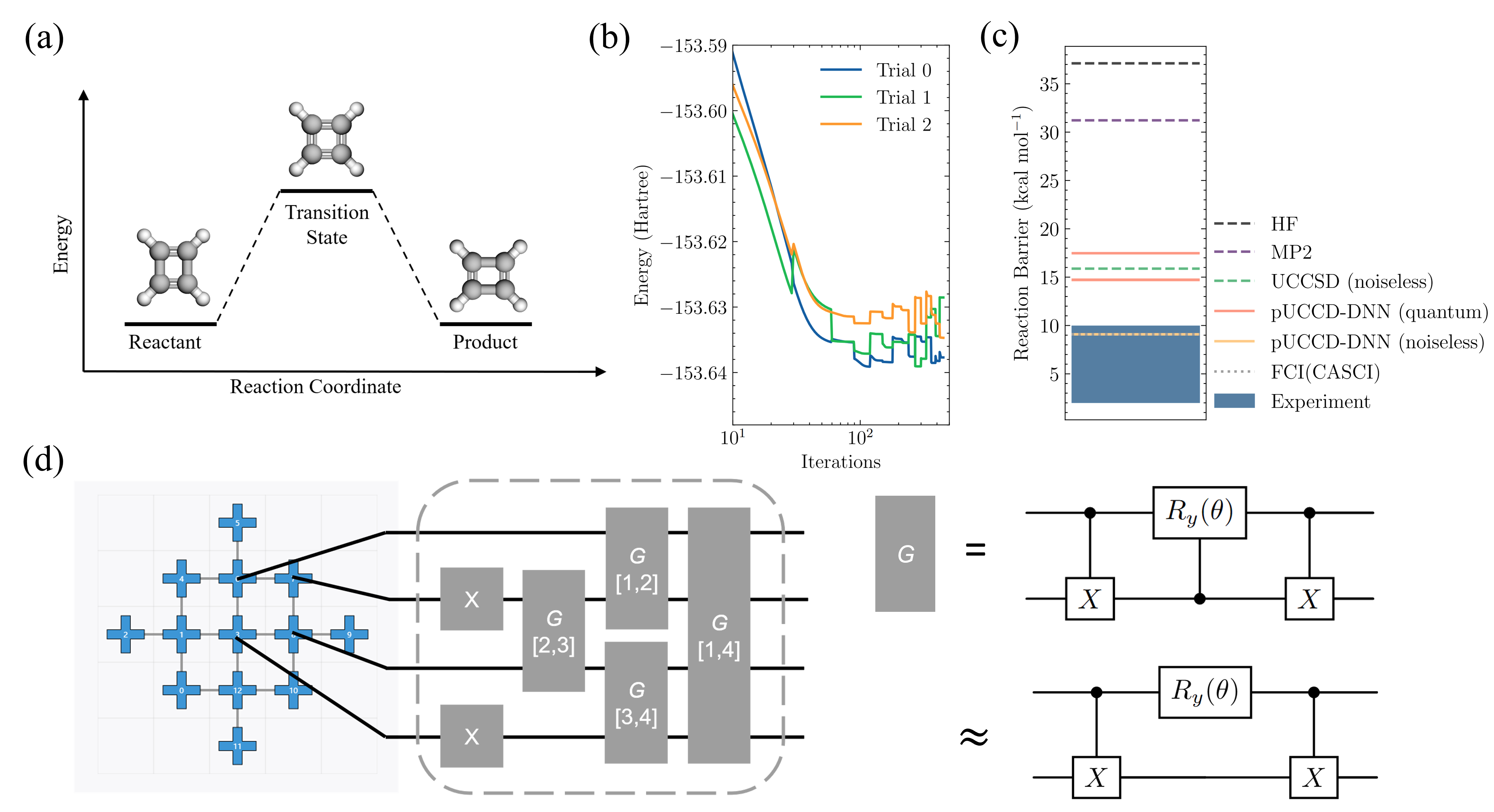
Figure 6: Experiments on a superconducting quantum computer. (a) The isomerization reaction of cyclobutadiene, with the transition state energy calculated using pUCCD-DNN on a superconducting quantum computer. (b) The estimated energy during the optimization process. Results by three independent random initializations of the neural network are shown. (c) The computed reaction barrier from pUCCD-DNN, compared with results from several other computational methods. “Experiment” means the reaction barrier calculated by experimentally observed chemical reaction rate.(d) The 13-qubit superconducting quantum chip and the quantum circuit used for the calculation.

Next, we investigate the advantage of incorporating quantum computing into the pUCCD-DNN framework. Since neural networks are widely known for their effectiveness across a variety of tasks including representing molecular wavefunction, it is important to assess whether a quantum circuit is truly necessary for this framework. To explore this, we use the transition state of the cyclobutadiene isomerization reaction as our model system. To highlight the role of the quantum circuit, we replace the pUCCD circuit in pUCCD-DNN with a Hadamard superposition circuit, where Hadamard gates are applied to all qubits. The Hadamard superposition circuit can be easily emulated on classical computers and can be considered as a “dummy” sample generator when used to compute the energy with the deep neural network. To isolate the impact of quantum gate noise, we perform the comparison using a shot-based classical emulator which is free of gate noise. As shown in Fig. 7, replacing the pUCCD circuit with a Hadamard superposition leads to a noticeable decrease in accuracy, along with a significant increase in energy variance. In fact, for large molecules, a Hadamard superposition circuit greatly reduces the probability of sampling the dominant configuration, making it less effective for energy estimation. In contrast, the pUCCD circuit provides a strong starting point for further refinement through deep neural network training, demonstrating the advantage of quantum computing in this context.

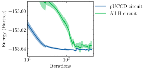
Figure 7: Energy estimates during neural network training with different quantum circuits. This figure illustrates the effect of quantum circuits on energy estimation within the pUCCD-DNN framework: (1) the pUCCD circuit, which is the circuit used throughout this paper, and (2) the Hadamard superposition circuit, where Hadamard gates are applied to all qubits, creating a superposition of all possible states. The standard deviation across five different neural network initializations is shown as the shaded area.

III Discussion

The pUCCD-DNN framework combines an efficient quantum circuit with the expressive power of deep neural networks to accurately and robustly compute quantum molecular energies. By integrating a carefully designed algorithmic structure—including the pUCCD circuit, entanglement circuit, perturbation circuit, and neural network augmentation—the method achieves low quantum resource requirements, utilizing only $N$ qubits instead of the $2N$ qubits typically required by comparable methods. The design also ensures manageable measurement overhead for the interaction between the quantum circuit and the neural network.

Extensive numerical benchmarks demonstrate that pUCCD-DNN achieves accuracy comparable to advanced methods like UCCSD, while being more resource-efficient and scalable to larger molecular systems. The incorporation of a deep neural network, optimized via the variational principle, allows the framework to mitigate errors effectively, making it robust to gate noise and capable of delivering consistent accuracy on noisy quantum hardware.

Experimental validation on a superconducting quantum computer demonstrates the practicality of this approach. A 4-qubit quantum circuit with eight CNOT gates was successfully used to compute the transition state of cyclobutadiene isomerization, yielding energy estimates with accuracy comparable to noiseless UCCSD. Based on this model reaction, we also demonstrate that the quantum circuit plays an indispensable role in the hybrid framework, as replacing it with a neural network alone leads to a higher error and, crucially, a significantly larger variance in energy estimation.

While this work focuses on closed-shell systems, the pUCCD-DNN framework can be directly extended to open-shell systems by modifying the particle number conservation mask in the neural network. However, since the pUCCD quantum circuit may not accurately approximate open-shell wavefunctions, further adaptations will likely be necessary to maintain accuracy for open-shell systems. Future work could enhance the neural network architecture by incorporating more sophisticated neural layers with physical insights. Additionally, pretraining the neural network on a diverse set of molecules offers a possible avenue for creating a generalizable model that can be fine-tuned for specific systems.

IV Methods

IV.1 The electronic structure problem and the pUCCD ansatz

In this work, we are interested in the second-quantized ab initio electronic structure Hamiltonian

$$\hat{H}=\sum_{pq}h_{pq}\hat{a}^{\dagger}_{p}\hat{a}_{q}+\frac{1}{2}\sum_{pqrs}h_{pqrs}\hat{a}^{\dagger}_{p}\hat{a}^{\dagger}_{q}\hat{a}_{r}\hat{a}_{s}+E_{\rm{nuc}},\$$ (17)

where $h_{pq}$ and $h_{pqrs}=[ps|qr]$ are one-electron and two-electron integrals, and $\hat{a}^{\dagger}_{p},\hat{a}_{p}$ are fermionic creation and annihilation operators, respectively, acting on the $p$-th spin-orbital.

In order to compute the expectation of Eq. (17) on a quantum computer, the symmetry of the creation and annihilation operators has to be taken care of. creation and annihilation operators for fermions obey the anticommutation relations

$$\{\hat{a}_{i},\hat{a}^{\dagger}_{j}\} =\delta_{ij}$$ (18)

$$\{\hat{a}^{\dagger}_{i},\hat{a}^{\dagger}_{j}\} =\{\hat{a}_{i},\hat{a}_{j}\}=0$$

On the other hand, the qubit creation operator $\hat{c}^{\dagger}=\frac{1}{2}(X-iY)$ and annihilation operator $\hat{c}=\frac{1}{2}(X+iY)$ obey the commutation relations

$$\{\hat{c}_{i},\hat{c}^{\dagger}_{j}\}=\delta_{ij},\quad[\hat{c}^{\dagger}_{i},\hat{c}^{\dagger}_{j}]=[\hat{c}_{i},\hat{c}_{j}]=0.$$ (19)

In this work, when necessary, we employ the Jordan-Wigner transformation to map fermionic ladder operators into qubit operators

In general, UCC types of ansatzes can be written as

$$\ket{\Psi(\theta)}_{\text{UCC}}:=\prod e^{\theta_{k}\hat{G}_{k}}\ket{\phi}.\$$ (20)

Here, $\ket{\phi}=\ket{\text{HF}}$ is the Hartree–Fock state. For the UCCSD method in this work, $\hat{G}_{k}$ has the form

$$\hat{G}_{k}=\begin{cases}\hat{a}^{\dagger}_{p}\hat{a}_{q}-\text{h.c.},\\ \hat{a}^{\dagger}_{p}\hat{a}^{\dagger}_{q}\hat{a}_{r}\hat{a}_{s}-\text{h.c.}\end{cases}$$ (21)

pUCCD is an efficient ansatz requiring only $\order{N}$ circuit depth and half as many qubits as other UCC ansatze [28, 29]. pUCCD allows only paired double excitations, which enables one qubit to represent one spatial orbital instead of one spin orbital, and removes the need to perform the fermion-qubit mapping. The subspace in which all states have paired configuration is called the seniority-zero subspace. In this subspace, there are $\order{N^{2}}$ double excitations, which can be executed on a quantum computer efficiently using a compact circuit. The circuit is composed of a linear depth of Givens-SWAP gates, assuming linear qubit connectivity [29]. In the seniority-zero subspace, the Hamiltonian also takes a simpler form, with only $N^{2}$ terms:

$$\hat{H}=\sum_{p}h_{p}\hat{c}^{\dagger}_{p}\hat{c}_{p}+\sum_{pq}v_{pq}\hat{c}^{\dagger}_{p}\hat{c}_{q}+\sum_{p\neq q}w_{pq}\hat{c}^{\dagger}_{p}\hat{c}_{p}\hat{c}^{\dagger}_{q}\hat{c}_{q}+E_{\rm{nuc}}\ ,$$ (22)

where $h_{p}=2h_{pp}$, $v_{pq}=(pq|pq)$ and $\omega_{pq}=2(pp|qq)-(pq|pq)$. Here $p$ and $q$ are indices for spatial orbitals. If we use $\hat{n}_{p}=\hat{c}^{\dagger}_{p}\hat{c}_{p}=\frac{1-Z}{2}$ to denote occupation number operator, Eq. (22) can be converted to a sum of Pauli string where the maximum length of Pauli string is 2. Meanwhile, the first and the third term in Eq. (22) have only $Z$ terms and the second term will contribute to $XX$ and $YY$ terms. Thus, the expectation of Eq. (22) can be measured in 3 different bases, regardless the number of qubit involved.

IV.2 The measurement protocol for pUCCD-DNN

IV.2.1 A single quantum circuit

To begin with, we describe the measurement protocol when a single quantum circuit is integrated with a deep neural network, following the reference [46]. Then, we move on to our measurement method that enables efficient measurement of two separate circuits in the pUCCD-DNN algorithm, defined in Eq. (16). In the following, for clarity, we omit the prime symbol for both $\hat{H}^{\prime}$ and $\hat{N}^{\prime}$, since $\hat{H}^{\prime}$ is Pauli string similar to $\hat{H}$, and $\hat{N}^{\prime}$ follows the definition of $\hat{N}$ in Eq. (5).

For a single circuit $\ket{\psi}=\sum_{k}a_{k}\ket{k}$, where $\ket{k}$ is the computational basis, $\hat{N}$ is written as

$$\hat{N}=\sum_{k}b_{k}\ket{k}\bra{k}\ .$$ (23)

We then focus on deriving an appropriate form of $\hat{N}\hat{H}\hat{N}$. We assume that both $\ket{\psi}$ and $\hat{N}$ are real-valued. We first derive the measurement protocol for the norm of $\ket{\Psi}=\hat{N}\ket{\psi}$. The norm of $\ket{\Psi}$ is given by

$$\braket{\Psi|\Psi}=\braket{\psi|\hat{N}^{\dagger}\hat{N}|\psi}\ ,$$ (24)

where

$$\hat{N}^{\dagger}\hat{N}=\sum_{k}b_{k}^{2}\ket{k}\bra{k}\ .$$ (25)

Clearly, the eigenvectors of $\hat{N}^{\dagger}\hat{N}$ are $\ket{k}$ and their eigenvalues are $b^{2}_{k}$. To compute the norm, we sample bitstrings from $\ket{\psi}$ and multiply the probability of $k$ by $b^{2}_{k}$. For efficient sampling, $b_{k}$ should not be too large or small. In other words, $a_{k}$ must provide a good first-order approximation to the ground state. The same is also true for our measurement protocol for 2 circuits and it highlights the role of the quantum computer in this framework.

Next, we consider the measurement of a Pauli string $\hat{H}$. The main focus is to derive $\hat{N}^{\dagger}\hat{H}\hat{N}$.

In general, a Pauli string $\hat{H}$ can be written as

$$\hat{H}=\sum_{k}S_{\tilde{k}}\ket{{\tilde{k}}}\bra{k}\ ,$$ (26)

where the summation is over $k$ rather than $k$ and ${\tilde{k}}$. In other words, applying the Pauli string $\hat{H}$ on $\ket{k}$ will produce only one bitstring $\ket{{\tilde{k}}}$

$$\hat{H}\ket{k}=S_{{\tilde{k}}}\ket{{\tilde{k}}}\ .$$ (27)

Since $\hat{H}^{2}=I$, we also have $\hat{H}\ket{{\tilde{k}}}=S_{k}\ket{k}$ and $S_{{\tilde{k}}}S_{k}=1$.

Let’s first consider the case where $\hat{H}$ has only $Z$ operators, i.e. $\ket{k}=\ket{{\tilde{k}}}$. In this case, the term to measure is

$$\hat{N}^{\dagger}\hat{H}\hat{N}=\sum_{k}b_{k}^{2}S_{k}\ket{k}\bra{k}\ .$$ (28)

Eq. (28) is similar to the expression for $\hat{N}^{\dagger}\hat{N}$ in Eq. (25). As a result, the measurement protocol when $\hat{H}$ only involves $Z$ operators is very similar to the procedure for measuring the norm of the state.

Now, consider the general case where $\hat{H}$ includes at least one $X$ or $Y$ operator, where it is ensured that $\ket{k}\neq\ket{{\tilde{k}}}$. In this case, we can rewrite $\hat{H}$ as

$$\hat{H}=\sum_{k\in\Omega}\left(S_{k}\ket{k}\bra{{\tilde{k}}}+S_{\tilde{k}}\ket{{\tilde{k}}}\bra{k}\right)\ ,$$ (29)

where $\Omega=\{k|\textrm{bin}(k)<\textrm{bin}({\tilde{k}})\}$ and $\textrm{bin}(k)$ refers to the corresbonding binary integer of $k$.

The Hamiltonian transformed by $\hat{N}$ is given by

$$\hat{N}^{\dagger}\hat{H}\hat{N}=\sum_{k\in\Omega}b_{k}b_{\tilde{k}}\hat{H}_{k}\ ,$$ (30)

where

$$\hat{H}_{k}=S_{k}\ket{k}\bra{{\tilde{k}}}+S_{\tilde{k}}\ket{{\tilde{k}}}\bra{k}\ .$$ (31)

To measure $\hat{N}^{\dagger}\hat{H}\hat{N}$, we need to derive the eigenvectors of $\hat{H}_{k}$. $\hat{H}_{k}$ is defined by two basis $\ket{k}$ and $\ket{{\tilde{k}}}$ and therefore $\hat{H}_{k}$ has two eigenvectors with eigenvalues +1 and -1. Denote the two eigenvectors as $\ket{k^{+}}$ and $\ket{k^{-}}$, we can then write $\hat{H}_{k}$ as

$$\hat{H}_{k}=\ket{k^{+}}\bra{k^{+}}-\ket{k^{-}}\bra{k^{-}}\ .$$ (32)

In the computational basis, $\ket{k^{+}}$ and $\ket{k^{-}}$ are written as

$$\sqrt{2}\ket{k^{+}}=S_{\tilde{k}}\ket{{\tilde{k}}}+\ket{k}=(\hat{H}_{k}+1)\ket{k}\ ,$$ (33)

$$\sqrt{2}\ket{k^{-}}=S_{\tilde{k}}\ket{{\tilde{k}}}-\ket{k}=(\hat{H}_{k}-1)\ket{k}\ .$$

These eigenvectors have eigenvalues $+1$ and $-1$, respectively. The DNN transformed Hamiltonian is then

$$\hat{N}^{\dagger}\hat{H}\hat{N}=\sum_{k\in\Omega}b_{k}b_{\tilde{k}}\left(\ket{k^{+}}\bra{k^{+}}-\ket{k^{-}}\bra{k^{-}}\right)\ .$$ (34)

Next we need to perform the measurement in the $\ket{k^{+}}$ and $\ket{k^{-}}$ bases. To achieve this, we append a unitary measurement circuit $V$ to the original quantum circuit $\ket{\psi}$ which satisfies

$$V^{\dagger}\ket{k}=\ket{k^{+}}\ ,$$ (35)

$$V^{\dagger}\ket{{\tilde{k}}}=\ket{k^{-}}\ ,$$

for any $k\in\Omega$. The unitary property can be proven by considering $\braket{k^{\prime}|VV^{\dagger}|k}$ or by noting that $V$ is a permutation between two sets of orthonormal basis states. The construction of the transformation circuit $\hat{V}$ is a standard procedure in quantum information. Essentially, $\hat{V}$ is a circuit that diagonalizes the Pauli string $\hat{H}$. If the number of $X$ and $Y$ operators in $\hat{H}$ is $m$, then the number of two-qubit gates in $\hat{V}$ is $m-1$.

To summarize, the quantum circuit used for the measurement is $\hat{V}\ket{\psi}$, and the term to measure is

$$\hat{V}\hat{N}^{\dagger}\hat{H}\hat{N}\hat{V}^{\dagger}=\sum_{k\in\Omega}b_{k}b_{\tilde{k}}\left(\ket{k}\bra{k}-\ket{{\tilde{k}}}\bra{{\tilde{k}}}\right)\ .$$ (36)

The expectation value of this term is readily accessible from the quantum circuit $\hat{V}\ket{\psi}$ by performing a projection measurement in the computational basis.

IV.2.2 Two separate quantum circuits

If we take the two separate quantum circuit $\ket{\psi\otimes\phi}$ as a whole, the measurement protocol developed in Sec. IV.2.1 can be applied to measure the expectation when a deep neural network is integrated with $\ket{\psi\otimes\phi}$. However, in this case, the unitary transformation for measurement $V$ will generally entangle the two originally unentangled quantum circuits. This results in a quantum circuit of $2N$ qubits. If we wish to avoid this entanglement and measure the expectation using two separate quantum circuits, a special measurement procedure is needed. This procedure will be described in the following.

The total wavefunction can be expressed as:

$$\ket{\Psi}=\hat{N}\ket{\psi\otimes\phi}\ .$$ (37)

In our pUCCD-DNN framework, $\ket{\psi}$ is the pUCCD quantum circuit, and $\ket{\phi}$ is the perturbation circuit to be simulated classically. However, our procedure outlined below is general and can be readily applied to other cases involving uncorrelated circuits.

Consider Hamiltonian in the form:

$$\hat{H}=\hat{H}_{\psi}\otimes\hat{H}_{\phi}\ ,$$ (38)

where $\hat{H}_{\psi}$ and $\hat{H}_{\phi}$ are Pauli strings for the two separate circuits. If either of $\hat{H}_{\psi}$ and $\hat{H}_{\phi}$ does not contain $X$ or $Y$, the measurement procedure simplifies to the standard approach described in Sec. IV.2.1. Therefore, we will focus on the general case where both $\hat{H}_{\psi}$ and $\hat{H}_{\phi}$ contain $X$ or $Y$. Similar to Eq. (27), $\hat{H}_{\psi}$ and $\hat{H}_{\phi}$ satisfy the following relations:

$$\hat{H}_{\psi}\ket{k} =S_{{\tilde{k}}}\ket{{\tilde{k}}}\ ,$$ (39)

$$\hat{H}_{\phi}\ket{j} =S_{{\tilde{j}}}\ket{{\tilde{j}}}\ .$$

Here, $\hat{H}_{\psi}$ and $\hat{H}_{\phi}$ act independently on the circuit $\ket{\psi}$ and $\ket{\phi}$, transforming the states $\ket{k}$ and $\ket{j}$ into $\ket{{\tilde{k}}}$ and $\ket{{\tilde{j}}}$, with corresponding signs $S_{{\tilde{k}}}$ and $S_{{\tilde{j}}}$.

The eigenvectors of $\hat{H}$ are given by

$$2\ket{k^{\pm}}\ket{j^{\pm}}=\left(S_{{\tilde{k}}}\ket{{\tilde{k}}}\pm\ket{k}\right)\left(S_{{\tilde{j}}}\ket{{\tilde{j}}}\pm\ket{j}\right)\ ,$$ (40)

where we again require $k\in\Omega_{\psi}$ and $j\in\Omega_{\phi}$ to avoid double-counting. In the following, we use $k,j\in\Omega$ as a short-hand notation for the condition.

The Hamiltonian in the computational basis is

$$\hat{H} =\sum_{k,j\in\Omega}\left(S_{k}\ket{k}\bra{{\tilde{k}}}+S_{{\tilde{k}}}\ket{{\tilde{k}}}\bra{k}\right)\otimes\left(S_{j}\ket{j}\bra{{\tilde{j}}}+S_{{\tilde{j}}}\ket{{\tilde{j}}}\bra{j}\right)$$ (41)

$$=\sum_{k,j\in\Omega}\left(S_{k}S_{j}\ket{k,j}\bra{{\tilde{k}},{\tilde{j}}}+S_{{\tilde{k}}}S_{{\tilde{j}}}\ket{{\tilde{k}},{\tilde{j}}}\bra{k,j}\right)$$

$$\quad+\sum_{k,j\in\Omega}\left(S_{k}S_{{\tilde{j}}}\ket{k,{\tilde{j}}}\bra{{\tilde{k}},j}+S_{{\tilde{k}}}S_{j}\ket{{\tilde{k}},j}\bra{k,{\tilde{j}}}\right)\ .$$

After applying the transformation $\hat{N}$, the transformed Hamiltonian becomes

$$\hat{N}^{\dagger}\hat{H}\hat{N} =\sum_{k,j\in\Omega}b_{k,j}b_{{\tilde{k}},{\tilde{j}}}\left(S_{k}S_{j}\ket{k,j}\bra{{\tilde{k}},{\tilde{j}}}+S_{{\tilde{k}}}S_{{\tilde{j}}}\ket{{\tilde{k}},{\tilde{j}}}\bra{k,j}\right)$$ (42)

$$\quad+\sum_{k,j\in\Omega}b_{k,{\tilde{j}}}b_{{\tilde{k}},j}\left(S_{k}S_{{\tilde{j}}}\ket{k,{\tilde{j}}}\bra{{\tilde{k}},j}+S_{{\tilde{k}}}S_{j}\ket{{\tilde{k}},j}\bra{k,{\tilde{j}}}\right)\ .$$

The structure of $\hat{N}^{\dagger}\hat{H}\hat{N}$ remains similar to $\hat{H}$, but the terms are now weighted by the neural network coefficients $b_{k,j}$.

Eq. (42) is more complex than Eq. (30) since each term can not be readily factored into the direct product of operators acting on the two separate circuits. Consequently, finding a measurement circuit that diagonalizes Eq. (42) without introducing entanglement between the two circuits is not straightforward.

To proceed, it is instructive to consider a 2-qubit system and with the Hamiltonian $\hat{H}=XX$ as an example. In this case, we can express the DNN transformed Hamiltonian as:

$$\hat{N}^{\dagger}\hat{H}\hat{N} =b_{00}b_{11}(\ket{00}\bra{11}+\ket{11}\bra{00})+b_{01}b_{10}(\ket{01}\bra{10}+\ket{10}\bra{01})$$ (43)

$$=\frac{1}{2}b_{00}b_{11}(XX-YY)+\frac{1}{2}b_{01}b_{10}(XX+YY)$$

$$=\frac{1}{2}(b_{00}b_{11}+b_{01}b_{10})XX+\frac{1}{2}(-b_{00}b_{11}+b_{01}b_{10})YY\ .$$

Thus, to measure the expectation value of $XX$ in the presence of a DNN, one needs to measure both $XX$ and $YY$ to avoid measurement circuit that entangles the two separate circuits.

More generally, consider a Hamiltonian $\hat{J}=\hat{J}_{\psi}\otimes\hat{J}_{\phi}$ such that (as in Eq. (39))

$$\hat{J}_{\psi}\ket{k} =iS_{{\tilde{k}}}\ket{{\tilde{k}}}\ ,$$ (44)

$$\hat{J}_{\phi}\ket{j} =iS_{{\tilde{j}}}\ket{{\tilde{j}}}\ .$$

$\hat{J}$ can be constructed by replacing an $X$ operator with $-Y$ or a $Y$ operator with $X$ in $\hat{H}_{\psi}$ and $\hat{H}_{\phi}$. The eigenvectors of $\hat{J}$ are

$$2\ket{k^{i\pm}}\ket{j^{i\pm}}=\left(iS_{{\tilde{k}}}\ket{{\tilde{k}}}\pm\ket{k}\right)\left(iS_{{\tilde{j}}}\ket{{\tilde{j}}}\pm\ket{j}\right)\ .$$ (45)

We define short-hand notation for the projectors

$$\hat{h}_{k}^{\pm}=\ket{k^{\pm}}\bra{k^{\pm}}\,$$ (46)

which form the diagonal bases for $\hat{H}$ and $\hat{J}$. The first term of $\hat{N}^{\dagger}\hat{H}\hat{N}$ from Eq. (42) is then transformed to:

$$S_{k}S_{j}\ket{k,j}\bra{{\tilde{k}},{\tilde{j}}}+S_{{\tilde{k}}}S_{{\tilde{j}}}\ket{{\tilde{k}},{\tilde{j}}}\bra{k,j}$$ (47)

$$=\frac{1}{2}(\hat{h}_{k}^{+}-\hat{h}_{k}^{-})\otimes(\hat{h}_{j}^{+}-\hat{h}_{j}^{-})-\frac{1}{2}(\hat{h}_{k}^{i+}-\hat{h}_{k}^{i-})\otimes(\hat{h}_{j}^{i+}-\hat{h}_{j}^{i-})\ .$$

Similarly, the second term becomes

$$S_{k}S_{{\tilde{j}}}\ket{k,{\tilde{j}}}\bra{{\tilde{k}},j}+S_{{\tilde{k}}}S_{j}\ket{{\tilde{k}},j}\bra{k,{\tilde{j}}}$$ (48)

$$=\frac{1}{2}(\hat{h}_{k}^{+}-\hat{h}_{k}^{-})\otimes(\hat{h}_{j}^{+}-\hat{h}_{j}^{-})+\frac{1}{2}(\hat{h}_{k}^{i+}-\hat{h}_{k}^{i-})\otimes(\hat{h}_{j}^{i+}-\hat{h}_{j}^{i-})\ .$$

The overall expression for $\hat{N}^{\dagger}\hat{H}\hat{N}$ is

$$\hat{N}^{\dagger}\hat{H}\hat{N} =\sum_{k,j\in\Omega}\frac{1}{2}\left(b_{k,j}b_{{\tilde{k}},{\tilde{j}}}+b_{k,{\tilde{j}}}b_{{\tilde{k}},j}\right)(\hat{h}_{k}^{+}-\hat{h}_{k}^{-})\otimes(\hat{h}_{j}^{+}-\hat{h}_{j}^{-})$$ (49)

$$\quad+\sum_{k,j\in\Omega}\frac{1}{2}\left(-b_{k,j}b_{{\tilde{k}},{\tilde{j}}}+b_{k,{\tilde{j}}}b_{{\tilde{k}},j}\right)(\hat{h}_{k}^{i+}-\hat{h}_{k}^{i-})\otimes(\hat{h}_{j}^{i+}-\hat{h}_{j}^{i-})$$

One may verify the equation by setting $b=1$ and $\hat{N}$ becomes $\hat{I}$. In this case, the second term vanishes and the first term reduces to the original Hamiltonian $\hat{H}$. In Eq. (49), the operators are factored into the direct product of operators acting on the two separate circuits. Consequently, they can be diagonalized to the computational basis separately following the approach discussed in Sec. IV.2.1.

Thus, in order to measure the expectation in Eq. (16), one has to sample bitstrings from both $\hat{H}$ and $\hat{J}$ and calculate the expectation following Eq. (49) accordingly. In the framework of pUCCD-DNN, we first sample bitstrings that correspond to $\hat{h}_{k}^{\pm}$ and $\hat{h}_{k}^{i\pm}$ on quantum computers, and then sample bitstrings that correspond to $\hat{h}_{j}^{\pm}$ and $\hat{h}_{j}^{i\pm}$ on classical simulators. Then we query the deep neural network $\mathcal{B}$ for $b_{k,j}$, and finally calculate the expectation based on the sampling statistics and the output from the deep neural network.

IV.3 Implementation of pUCCD-DNN

In the noiseless simulation described in Sec.II.2, we use the L-BFGS-B algorithm to optimize the parameters in the quantum circuit. For circuit optimization on real quantum hardware, we employ the SOAP method [63].

For both the noiseless simulations and the experiments on quantum computers, the deep neural network is trained using the AdaMax optimizer [66], a variant of the widely adopted Adam optimizer. The optimizer begins with a learning rate schedule of $\alpha=0.01$, $b_{1}=0.8$ and $b_{2}=0.99$. The learning rate decays linearly to $\alpha=0.001$ between the 8000th and 32000th steps. This learning rate schedule helps ensure stable convergence by gradually decreasing the learning rate as the training progresses. For noiseless simulation, the maximum number of steps is set to 64000. For the noiseless simulation, we initialize the deep neural network with five different random seeds, and the lowest energy found across these seeds is reported.

For quantum circuit manipulation, including both noiseless and noisy emulation as well as interfacing with real quantum hardware, we use the TensorCircuit framework [67]. Quantum computational chemistry tasks, including Hamiltonian construction, reference value calculation, and parameter optimization are handled by TenCirChem [68], a specialized package built on top of TensorCircuit designed for quantum computational chemistry. TenCirChem also relies on PySCF for evaluating the integrals and performing calculations based on classical computational chemistry [69].

Code Availability

The code for this study is available from the TenCirChem-NG package hosted on GitHub https://github.com/tensorcircuit/TenCirChem-NG.

References

- Lloyd [1996] S. Lloyd, Universal quantum simulators, Science 273, 1073 (1996).
- Daley et al. [2022] A. J. Daley, I. Bloch, C. Kokail, S. Flannigan, N. Pearson, M. Troyer, and P. Zoller, Practical quantum advantage in quantum simulation, Nature 607, 667 (2022).
- King et al. [2024] A. D. King, A. Nocera, M. M. Rams, J. Dziarmaga, R. Wiersema, W. Bernoudy, J. Raymond, N. Kaushal, N. Heinsdorf, R. Harris, et al., Computational supremacy in quantum simulation, arXiv preprint arXiv:2403.00910 (2024).
- Chan [2024] G. K.-L. Chan, Quantum chemistry, classical heuristics, and quantum advantage, Faraday Discuss. (2024).
- Preskill [2018] J. Preskill, Quantum Computing in the NISQ era and beyond, Quantum 2, 79 (2018).
- Bharti et al. [2022] K. Bharti, A. Cervera-Lierta, T. H. Kyaw, T. Haug, S. Alperin-Lea, A. Anand, M. Degroote, H. Heimonen, J. S. Kottmann, T. Menke, W.-K. Mok, S. Sim, L.-C. Kwek, and A. Aspuru-Guzik, Noisy intermediate-scale quantum algorithms, Rev. Mod. Phys. 94, 015004 (2022).
- Kim et al. [2023] Y. Kim, A. Eddins, S. Anand, K. X. Wei, E. Van Den Berg, S. Rosenblatt, H. Nayfeh, Y. Wu, M. Zaletel, K. Temme, et al., Evidence for the utility of quantum computing before fault tolerance, Nature 618, 500 (2023).
- Ni et al. [2023] Z. Ni, S. Li, X. Deng, Y. Cai, L. Zhang, W. Wang, Z.-B. Yang, H. Yu, F. Yan, S. Liu, et al., Beating the break-even point with a discrete-variable-encoded logical qubit, Nature 616, 56 (2023).
- Xu et al. [2024] Q. Xu, J. P. Bonilla Ataides, C. A. Pattison, N. Raveendran, D. Bluvstein, J. Wurtz, B. Vasić, M. D. Lukin, L. Jiang, and H. Zhou, Constant-overhead fault-tolerant quantum computation with reconfigurable atom arrays, Nat. Phys. 20, 1084 (2024).
- Bravyi et al. [2024] S. Bravyi, A. W. Cross, J. M. Gambetta, D. Maslov, P. Rall, and T. J. Yoder, High-threshold and low-overhead fault-tolerant quantum memory, Nature 627, 778 (2024).
- Bluvstein et al. [2024] D. Bluvstein, S. J. Evered, A. A. Geim, S. H. Li, H. Zhou, T. Manovitz, S. Ebadi, M. Cain, M. Kalinowski, D. Hangleiter, et al., Logical quantum processor based on reconfigurable atom arrays, Nature 626, 58 (2024).
- Quantum and Collaborators [2024] G. A. Quantum and Collaborators, Quantum error correction below the surface code threshold, arXiv preprint arXiv:2408.13687 (2024).
- Peruzzo et al. [2014] A. Peruzzo, J. McClean, P. Shadbolt, M.-H. Yung, X.-Q. Zhou, P. J. Love, A. Aspuru-Guzik, and J. L. O’brien, A variational eigenvalue solver on a photonic quantum processor, Nat. Commun. 5, 1 (2014).
- Cerezo et al. [2021] M. Cerezo, A. Arrasmith, R. Babbush, S. C. Benjamin, S. Endo, K. Fujii, J. R. McClean, K. Mitarai, X. Yuan, L. Cincio, and P. J. Coles, Variational quantum algorithms, Nat. Rev. Phys. 3, 625 (2021).
- Tilly et al. [2022] J. Tilly, H. Chen, S. Cao, D. Picozzi, K. Setia, Y. Li, E. Grant, L. Wossnig, I. Rungger, G. H. Booth, and J. Tennyson, The variational quantum eigensolver: a review of methods and best practices, Phys. Rep. 986, 1 (2022).
- LeCun et al. [2015] Y. LeCun, Y. Bengio, and G. Hinton, Deep learning, Nature 521, 436 (2015).
- Anand et al. [2022] A. Anand, P. Schleich, S. Alperin-Lea, P. W. Jensen, S. Sim, M. Díaz-Tinoco, J. S. Kottmann, M. Degroote, A. F. Izmaylov, and A. Aspuru-Guzik, A quantum computing view on unitary coupled cluster theory, Chem. Soc. Rev. 51, 1659 (2022).
- Kandala et al. [2017] A. Kandala, A. Mezzacapo, K. Temme, M. Takita, M. Brink, J. M. Chow, and J. M. Gambetta, Hardware-efficient variational quantum eigensolver for small molecules and quantum magnets, Nature 549, 242 (2017).
- Lee et al. [2018] J. Lee, W. J. Huggins, M. Head-Gordon, and K. B. Whaley, Generalized unitary coupled cluster wave functions for quantum computation, J. Chem. Theory Comput. 15, 311 (2018).
- Magoulas and Evangelista [2023] I. Magoulas and F. A. Evangelista, Linear-scaling quantum circuits for computational chemistry, J. Chem. Theory Comput. 19, 4815 (2023).
- Grimsley et al. [2019] H. R. Grimsley, S. E. Economou, E. Barnes, and N. J. Mayhall, An adaptive variational algorithm for exact molecular simulations on a quantum computer, Nat. Commun. 10, 3007 (2019).
- Kandala et al. [2019] A. Kandala, K. Temme, A. D. Córcoles, A. Mezzacapo, J. M. Chow, and J. M. Gambetta, Error mitigation extends the computational reach of a noisy quantum processor, Nature 567, 491 (2019).
- Gao et al. [2021a] Q. Gao, G. O. Jones, M. Motta, M. Sugawara, H. C. Watanabe, T. Kobayashi, E. Watanabe, Y.-y. Ohnishi, H. Nakamura, and N. Yamamoto, Applications of quantum computing for investigations of electronic transitions in phenylsulfonyl-carbazole TADF emitters, npj Comput. Mater. 7, 70 (2021a).
- Gao et al. [2021b] Q. Gao, H. Nakamura, T. P. Gujarati, G. O. Jones, J. E. Rice, S. P. Wood, M. Pistoia, J. M. Garcia, and N. Yamamoto, Computational investigations of the lithium superoxide dimer rearrangement on noisy quantum devices, J. Phys. Chem. A 125, 1827 (2021b).
- Kirsopp et al. [2022] J. J. Kirsopp, C. Di Paola, D. Z. Manrique, M. Krompiec, G. Greene-Diniz, W. Guba, A. Meyder, D. Wolf, M. Strahm, and D. Muñoz Ramo, Quantum computational quantification of protein-ligand interactions, Int. J. Quantum Chem. 122, e26975 (2022).
- McClean et al. [2018] J. R. McClean, S. Boixo, V. N. Smelyanskiy, R. Babbush, and H. Neven, Barren plateaus in quantum neural network training landscapes, Nat. Commun. 9, 4812 (2018).
- Sun et al. [2024] J. Sun, L. Cheng, and W. Li, Toward chemical accuracy with shallow quantum circuits: A Clifford-based Hamiltonian engineering approach, J. Chem. Theory Comput. 20, 695 (2024).
- Henderson et al. [2015] T. M. Henderson, I. W. Bulik, and G. E. Scuseria, Pair extended coupled cluster doubles, J. Chem. Phys. 142, 214116 (2015).
- Elfving et al. [2021] V. E. Elfving, M. Millaruelo, J. A. Gámez, and C. Gogolin, Simulating quantum chemistry in the seniority-zero space on qubit-based quantum computers, Phys. Rev. A 103, 032605 (2021).
- O’Brien et al. [2023] T. E. O’Brien, G. Anselmetti, F. Gkritsis, V. E. Elfving, S. Polla, W. J. Huggins, O. Oumarou, K. Kechedzhi, D. Abanin, R. Acharya, I. Aleiner, R. Allen, T. I. Andersen, K. Anderson, M. Ansmann, F. Arute, K. Arya, A. Asfaw, J. Atalaya, J. C. Bardin, A. Bengtsson, G. Bortoli, A. Bourassa, J. Bovaird, L. Brill, M. Broughton, B. Buckley, D. A. Buell, T. Burger, B. Burkett, N. Bushnell, J. Campero, Z. Chen, B. Chiaro, D. Chik, J. Cogan, R. Collins, P. Conner, W. Courtney, A. L. Crook, B. Curtin, D. M. Debroy, S. Demura, I. Drozdov, A. Dunsworth, C. Erickson, L. Faoro, E. Farhi, R. Fatemi, V. S. Ferreira, L. Flores Burgos, E. Forati, A. G. Fowler, B. Foxen, W. Giang, C. Gidney, D. Gilboa, M. Giustina, R. Gosula, A. Grajales Dau, J. A. Gross, S. Habegger, M. C. Hamilton, M. Hansen, M. P. Harrigan, S. D. Harrington, P. Heu, M. R. Hoffmann, S. Hong, T. Huang, A. Huff, L. B. Ioffe, S. V. Isakov, J. Iveland, E. Jeffrey, Z. Jiang, C. Jones, P. Juhas, D. Kafri, T. Khattar, M. Khezri, M. Kieferová, S. Kim, P. V. Klimov, A. R. Klots, A. N. Korotkov, F. Kostritsa, J. M. Kreikebaum, D. Landhuis, P. Laptev, K.-M. Lau, L. Laws, J. Lee, K. Lee, B. J. Lester, A. T. Lill, W. Liu, W. P. Livingston, A. Locharla, F. D. Malone, S. Mandrà, O. Martin, S. Martin, J. R. McClean, T. McCourt, M. McEwen, X. Mi, A. Mieszala, K. C. Miao, M. Mohseni, S. Montazeri, A. Morvan, R. Movassagh, W. Mruczkiewicz, O. Naaman, M. Neeley, C. Neill, A. Nersisyan, M. Newman, J. H. Ng, A. Nguyen, M. Nguyen, M. Y. Niu, S. Omonije, A. Opremcak, A. Petukhov, R. Potter, L. P. Pryadko, C. Quintana, C. Rocque, P. Roushan, N. Saei, D. Sank, K. Sankaragomathi, K. J. Satzinger, H. F. Schurkus, C. Schuster, M. J. Shearn, A. Shorter, N. Shutty, V. Shvarts, J. Skruzny, W. C. Smith, R. D. Somma, G. Sterling, D. Strain, M. Szalay, D. Thor, A. Torres, G. Vidal, B. Villalonga, C. Vollgraff Heidweiller, T. White, B. W. K. Woo, C. Xing, Z. J. Yao, P. Yeh, J. Yoo, G. Young, A. Zalcman, Y. Zhang, N. Zhu, N. Zobrist, D. Bacon, S. Boixo, Y. Chen, J. Hilton, J. Kelly, E. Lucero, A. Megrant, H. Neven, V. Smelyanskiy, C. Gogolin, R. Babbush, and N. C. Rubin, Purification-based quantum error mitigation of pair-correlated electron simulations, Nat. Phys. 19, 1787 (2023).
- Zhao et al. [2023a] L. Zhao, J. Goings, K. Shin, W. Kyoung, J. I. Fuks, J.-K. Kevin Rhee, Y. M. Rhee, K. Wright, J. Nguyen, J. Kim, et al., Orbital-optimized pair-correlated electron simulations on trapped-ion quantum computers, npj Quantum Inf. 9, 60 (2023a).
- Khan et al. [2023] I. Khan, M. Tudorovskaya, J. Kirsopp, D. Muñoz Ramo, P. Warrier, D. Papanastasiou, and R. Singh, Chemically aware unitary coupled cluster with ab initio calculations on an ion trap quantum computer: A refrigerant chemicals’ application, J. Chem. Phys. 158, 214114 (2023).
- Sokolov et al. [2020] I. O. Sokolov, P. K. Barkoutsos, P. J. Ollitrault, D. Greenberg, J. Rice, M. Pistoia, and I. Tavernelli, Quantum orbital-optimized unitary coupled cluster methods in the strongly correlated regime: Can quantum algorithms outperform their classical equivalents?, J. Chem. Phys. 152, 124107 (2020).
- Mizukami et al. [2020] W. Mizukami, K. Mitarai, Y. O. Nakagawa, T. Yamamoto, T. Yan, and Y.-y. Ohnishi, Orbital optimized unitary coupled cluster theory for quantum computer, Phys. Rev. Res. 2, 033421 (2020).
- Zhao et al. [2023b] L. Zhao, J. Goings, Q. Wang, K. Shin, W. Kyoung, S. Noh, Y. M. Rhee, and K. Kim, Enhancing the electron pair approximation with measurements on trapped ion quantum computers, arXiv preprint arXiv:2312.05426 (2023b).
- Windom et al. [2024] Z. W. Windom, D. Claudino, and R. J. Bartlett, An attractive way to correct for missing singles excitations in unitary coupled cluster doubles theory, arXiv preprint arXiv:2406.09174 (2024).
- Hermann et al. [2023] J. Hermann, J. Spencer, K. Choo, A. Mezzacapo, W. M. C. Foulkes, D. Pfau, G. Carleo, and F. Noé, Ab initio quantum chemistry with neural-network wavefunctions, Nat. Rev. Chem. 7, 692 (2023).
- Han et al. [2019] J. Han, L. Zhang, and E. Weinan, Solving many-electron schrödinger equation using deep neural networks, J. Comput. Phys. 399, 108929 (2019).
- Pfau et al. [2020] D. Pfau, J. S. Spencer, A. G. Matthews, and W. M. C. Foulkes, Ab initio solution of the many-electron schrödinger equation with deep neural networks, Phys. Rev. Res. 2, 033429 (2020).
- Hermann et al. [2020] J. Hermann, Z. Schätzle, and F. Noé, Deep-neural-network solution of the electronic schrödinger equation, Nat. Chem. 12, 891 (2020).
- Shang et al. [2023a] H. Shang, C. Guo, Y. Wu, Z. Li, and J. Yang, Solving schrödinger equation with a language model, arXiv preprint arXiv:2307.09343 (2023a).
- Li et al. [2022] X. Li, Z. Li, and J. Chen, Ab initio calculation of real solids via neural network ansatz, Nat. Commun. 13, 7895 (2022).
- Scherbela et al. [2024] M. Scherbela, L. Gerard, and P. Grohs, Towards a transferable fermionic neural wavefunction for molecules, Nat. Commun. 15, 120 (2024).
- Li et al. [2024a] X. Li, J.-C. Huang, G.-Z. Zhang, H.-E. Li, Z.-P. Shen, C. Zhao, J. Li, and H.-S. Hu, Improved optimization for the neural-network quantum states and tests on the chromium dimer, J. Chem. Phys. 160, 234102 (2024a).
- Nys et al. [2024] J. Nys, G. Pescia, and G. Carleo, Ab-initio variational wave functions for the time-dependent many-electron schrödinger equation, arXiv preprint arXiv:2403.07447 (2024).
- Zhang et al. [2022] S.-X. Zhang, Z.-Q. Wan, C.-K. Lee, C.-Y. Hsieh, S. Zhang, and H. Yao, Variational quantum-neural hybrid eigensolver, Phys. Rev. Lett. 128, 120502 (2022).
- Biamonte et al. [2017] J. Biamonte, P. Wittek, N. Pancotti, P. Rebentrost, N. Wiebe, and S. Lloyd, Quantum machine learning, Nature 549, 195 (2017).
- Cerezo et al. [2022] M. Cerezo, G. Verdon, H.-Y. Huang, L. Cincio, and P. J. Coles, Challenges and opportunities in quantum machine learning, Nature Comput. Sci. 2, 567 (2022).
- Ren et al. [2022] W. Ren, W. Li, S. Xu, K. Wang, W. Jiang, F. Jin, X. Zhu, J. Chen, Z. Song, P. Zhang, et al., Experimental quantum adversarial learning with programmable superconducting qubits, Nature Comput. Sci. 2, 711 (2022).
- Li et al. [2024b] X.-K. Li, J.-X. Ma, X.-Y. Li, J.-J. Hu, C.-Y. Ding, F.-K. Han, X.-M. Guo, X. Tan, and X.-M. Jin, High-efficiency reinforcement learning with hybrid architecture photonic integrated circuit, Nat. Commun. 15, 1044 (2024b).
- Li and Kais [2021] J. Li and S. Kais, Quantum cluster algorithm for data classification, Mat. Theory 5, 1 (2021).
- Sajjan et al. [2021] M. Sajjan, S. H. Sureshbabu, and S. Kais, Quantum machine-learning for eigenstate filtration in two-dimensional materials, J. Am. Chem. Soc. 143, 18426 (2021).
- Sajjan et al. [2022] M. Sajjan, J. Li, R. Selvarajan, S. H. Sureshbabu, S. S. Kale, R. Gupta, V. Singh, and S. Kais, Quantum machine learning for chemistry and physics, Chem. Soc. Rev. 51, 6475 (2022).
- Zeng et al. [2023] X. Zeng, Y. Fan, J. Liu, Z. Li, and J. Yang, Quantum neural network inspired hardware adaptable ansatz for efficient quantum simulation of chemical systems, J. Chem. Theory Comput. 19, 8587 (2023).
- Halder et al. [2024] S. Halder, A. Dey, C. Shrikhande, and R. Maitra, Machine learning assisted construction of a shallow depth dynamic ansatz for noisy quantum hardware, Chem. Sci. 15, 3279 (2024).
- Shang et al. [2024] H. Shang, X. Zeng, M. Gong, Y. Wu, S. Guo, H. Qian, C. Zha, Z. Fan, K. Yan, X. Zhu, Z. Li, Y. Luo, J.-W. Pan, and J. Yang, Rapidly achieving chemical accuracy with quantum computing enforced language model, arXiv preprint arXiv:2405.09164 (2024).
- Mazzola et al. [2019] G. Mazzola, P. J. Ollitrault, P. K. Barkoutsos, and I. Tavernelli, Nonunitary operations for ground-state calculations in near-term quantum computers, Phys. Rev. Lett. 123, 130501 (2019).
- Benfenati et al. [2021] F. Benfenati, G. Mazzola, C. Capecci, P. K. Barkoutsos, P. J. Ollitrault, I. Tavernelli, and L. Guidoni, Improved accuracy on noisy devices by nonunitary variational quantum eigensolver for chemistry applications, J. Chem. Theory Comput. 17, 3946 (2021).
- Shang et al. [2023b] Z.-X. Shang, M.-C. Chen, X. Yuan, C.-Y. Lu, and J.-W. Pan, Schrödinger-Heisenberg variational quantum algorithms, Phys. Rev. Lett. 131, 060406 (2023b).
- Zhang et al. [2023a] S. Zhang, Z.-Q. Wan, C.-Y. Hsieh, H. Yao, and S. Zhang, Variational Quantum‐Neural Hybrid Error Mitigation, Adv. Quantum Technol. 6, 202300147 (2023a).
- Lyakh et al. [2012] D. I. Lyakh, M. Musiał, V. F. Lotrich, and R. J. Bartlett, Multireference nature of chemistry: The coupled-cluster view, Chem. Rev. 112, 182 (2012).
- Dunning [1989] T. H. Dunning, Gaussian basis sets for use in correlated molecular calculations. I. the atoms boron through neon and hydrogen, J. Chem. Phys. 90, 1007 (1989).
- Li et al. [2024c] W. Li, Y. Ge, S.-X. Zhang, Y.-Q. Chen, and S. Zhang, Efficient and robust parameter optimization of the unitary coupled-cluster ansatz, J. Chem. Theory Comput. 20, 3683 (2024c).
- Whitman and Carpenter [1982] D. W. Whitman and B. K. Carpenter, Limits on the activation parameters for automerization of cyclobutadiene-1, 2-, J. Am. Chem. Soc. 104, 6473 (1982).
- Martens and Grosse [2015] J. Martens and R. Grosse, Optimizing neural networks with Kronecker-factored approximate curvature, in International conference on machine learning (PMLR, 2015) pp. 2408–2417.
- Kingma [2014] D. P. Kingma, Adam: A method for stochastic optimization, arXiv preprint arXiv:1412.6980 (2014).
- Zhang et al. [2023b] S.-X. Zhang, J. Allcock, Z.-Q. Wan, S. Liu, J. Sun, H. Yu, X.-H. Yang, J. Qiu, Z. Ye, Y.-Q. Chen, C.-K. Lee, Y.-C. Zheng, S.-K. Jian, H. Yao, C.-Y. Hsieh, and S. Zhang, Tensorcircuit: a quantum software framework for the NISQ era, Quantum 7, 912 (2023b).
- Li et al. [2023] W. Li, J. Allcock, L. Cheng, S.-X. Zhang, Y.-Q. Chen, J. P. Mailoa, Z. Shuai, and S. Zhang, TenCirChem: An efficient quantum computational chemistry package for the NISQ era, J. Chem. Theory Comput. 19, 3966 (2023).
- Sun et al. [2020] Q. Sun, X. Zhang, S. Banerjee, P. Bao, M. Barbry, N. S. Blunt, N. A. Bogdanov, G. H. Booth, J. Chen, Z.-H. Cui, et al., Recent developments in the PySCF program package, J. Chem. Phys. 153 (2020).