Target Tracking Using the
Invariant Extended Kalman Filter
with Adaptive Real-Time Numerical Differentiation for Estimating Curvature and Torsion
Target Tracking Using the
Invariant Extended Kalman Filter
with Numerical Differentiation for Estimating Curvature and Torsion
Target Tracking Using the Invariant Extended Kalman Filter
with Numerical Differentiation for Estimating Curvature and Torsion
Abstract
The goal of target tracking is to estimate target position, velocity, and acceleration in real time using position data. This paper introduces a novel target-tracking technique that uses adaptive input and state estimation (AISE) for real-time numerical differentiation to estimate velocity, acceleration, and jerk from position data. These estimates are used to model the target motion within the Frenet-Serret (FS) frame. By representing the model in SE(3), the position and velocity are estimated using the invariant extended Kalman filter (IEKF). The proposed method, called FS-IEKF-AISE, is illustrated by numerical examples and compared to prior techniques.
I INTRODUCTION
The goal of target tracking is to estimate target position, velocity, and acceleration in real time. As a key element in guidance, navigation, and control systems, target tracking relies on estimation algorithms that account for sensor noise and environmental effects. Numerous approaches have been developed to improve the accuracy and efficiency of these systems [1, 2, 3]. Simplifying assumptions, such as constant velocity and constant acceleration, are often invoked. When targets exhibit complex, unpredictable maneuvers, however, more sophisticated models are needed [4].
Prior research has explored various approaches for improving target tracking. [5] employs target acceleration predictions produced by a recurrent neural network for a predictive pursuer guidance algorithm. [6] discusses straight-line target tracking for unmanned surface vehicles using constant-bearing guidance to calculate a desired velocity. [7] presents a tracking scheme based on the Kalman filter, estimating acceleration inputs from residuals and updating the filter accordingly. [8] enhances real-time performance using vision-based state estimators for target tracking.
The extended Kalman filter (EKF) has been used to estimate the kinematic state of reentry ballistic targets, as shown by [9], while [10] uses the Kalman filter to track the movements of ballistic vehicles. Adaptive input estimation techniques for estimating the acceleration of maneuvering targets are demonstrated by [11, 12, 13]. [14] compares the performance and accuracy of EKF, unscented Kalman filter, and particle filter for tracking ballistic targets and predicting impact points using measurements from 3D radar.
Iterative solutions employing state transition matrices to correct the initial conditions of ballistic vehicles for trajectory calculation have been presented by [15]. To overcome the limitations of conventional constant-level maneuver models, [16, 17] propose a target-tracking technique using input estimation. [18] introduces a Kalman-filter-based tracking scheme incorporating input estimation for maneuvering targets. [19] proposes an intelligent Kalman filter for tracking maneuvering targets, using a fuzzy system optimized by genetic algorithms and DNA coding methods to compute timevarying process noise. Machine learning techniques, such as expert prediction, have also been applied to collaborative sensor network target tracking methods by [20].
The performance characterization of -- filters for constant-acceleration targets is discussed in [21], whereas [22] presents a procedure for selecting tracking parameters for all orders of tracking models. [23] provides an analytical expression for the tracking index, which is used for real-time applications. [24] presents an optimal reduced-state estimator for consistent tracking of maneuvering targets, addressing the limitations found in Kalman filters and interacting multiple model estimators commonly used for this purpose. The accuracy of these methods depends on the -- parameter values. To facilitate the selection of these parameters, [25] proposes an adaptive - filter, where the - parameters are adjusted in real-time using genetic algorithms.
Recent advances in target tracking focus on improving estimation accuracy for highly maneuvering targets in 3D spaces. [26] explores using the Frenet-Serret frame with the invariant extended Kalman filter (IEKF) [27] to track target motion using only position measurements under assumptions of constant speed, curvature, and torsion. [28] applied IEKF to air traffic control, while [29] extended the Frenet-Serret and Bishop frames within the IEKF framework to handle accelerating targets. However, these approaches struggle when the target trajectory, i.e., curvature, torsion, or speed, varies over time, representing realistic and complex maneuvers. Additionally, for a state space that consists of both Lie group and vector variables, [26, 30, 29] apply IEKF to a proper subset of the state space [26].
The contribution of this paper is a target-tracking technique that extends existing methods by removing the assumptions of constant speed, curvature, and torsion [26, 30, 29]. Unlike [26], the state space of the proposed approach is entirely modeled in SE(3), enabling the full application of IEKF. Furthermore, we use the Frenet-Serret (FS) formulas to compute timevarying estimates of speed, curvature, and torsion. These estimates require the velocity, acceleration, and jerk of the target, which are obtained using adaptive input and state estimation (AISE) for real-time numerical differentiation. The speed, curvature, and torsion are used by IEKF to filter the position measurements and estimate velocity. Numerical examples are provided to compare the performance of the proposed method FS-IEKF-AISE with FS-IEKF developed in [26].
II Problem Statement and Target Model
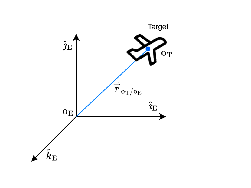
Consider a target moving in the 3D space with is any point fixed on the target. We assume that the Earth is inertially non-accelerating and non-rotating. The right-handed frame is fixed relative to the Earth, with the origin located at any convenient point on the Earth’s surface; hence, has zero inertial acceleration. points downward, and and are horizontal. is any point fixed on the target.
The location of the target origin relative to is represented by the position vector , as shown in Figure 1. We assume that a sensor measures the position of the target in the frame as
| (1) |
where is the step and . Here, is the position measurements of the target moving along a trajectory at step , with being the sample time.
The first, second, and third derivatives of with respect to represent the physical velocity, acceleration, and jerk vector , , and . Resolving , , and in yields
| (2) |
| (3) |
| (4) |
Given that the target moves along a trajectory , in 3D space, we model target trajectory using Frenet-Serret formulas as
| (5) |
where is the unit tangent vector and is the speed along . The Frenet-Serret formulas are given by
| (6) | ||||
| (7) | ||||
| (8) |
where is the curvature, is the torsion, and and are the unit normal and unit binormal vectors.
The vectors , and are mutually orthogonal. For brevity, the time variable will be omitted henceforth. The Frenet-Serret formulas (6), (7), and (8), can be written as [26]
| (9) |
Defining and , we write (9) as
| (10) |
Using the position, velocity, and acceleration defined by (1), (2), and (3), the tangent, normal, and binormal vectors at step are given by (excluding nongeneric cases) [31]
| (11) | ||||
| (12) | ||||
| (13) |
where , and Similarly, , , and at step are given by [31]
| (14) | ||||
| (15) | ||||
| (16) |
where , Note
| (17) | ||||
| (18) |
where and .
III Invariant Extended Kalman Filter (IEKF)
In this section, we present the novel invariant extended Kalman filter (IEKF) [27, 34] for the tracking problem on Lie group SE(3) using only position measurement. To model the target in an intrinsic coordinate system based on the Frenet-Serret frame, we define the orthogonal matrix
| (19) |
Under the assumption velocity vector and the tangent vector are colinear, the target dynamics using (5) and (10) are written as
| (20) | ||||
| (21) |
where , , denotes a skew-symmetric matrix, and are the white process noise. Note that the process noise for the position is only added in the tangential direction, that is, , where is white noise [30, 29].
Using the Lie group , which represents the group of 3D rotations and translations, we define
| (22) |
Rewriting the (20) and (21) using the Lie group framework [29, 26, 30]
| (23) |
where, for the Lie algebra , , , and
| (24) |
The noisy position measurement at step from a sensor is
| (25) |
where is Gaussian sensor noise with variance .
IEKF [27, 29, 34, 26] is applied to the target model (23). The evolution of the in (23) follows a symmetrical property
| (26) |
with satisfying
| (27) |
for all , where is an input variable and is the identity element in . This shows that (26) represents a group-affine system. Additional details are given in [27, 26].
The system (20) and (21) can be written in the form of (26) with
| (28) |
| (29) |
and the measurement (25) is rewritten as
| (30) |
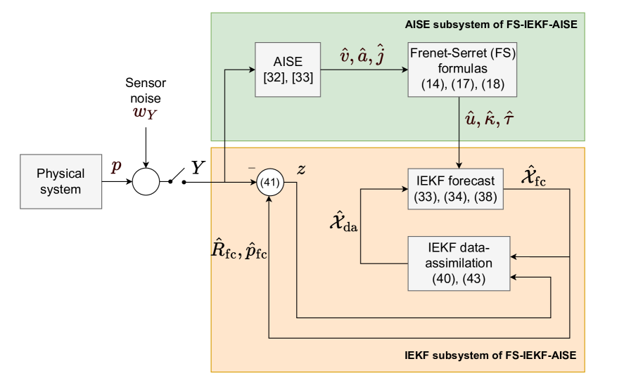
We treat and as external inputs to the system in (28), as shown in the block diagram of FS-IEKF-AISE in Figure 2 below.
Similar to the conventional Kalman filter, IEKF consists of two steps, namely, the forecast step and the data assimilation step. In discrete time, the forecast step, assuming the zero-order hold between and is [34]
| (31) | ||||
| (32) | ||||
| (33) | ||||
| (34) | ||||
| (35) |
where , , and are the data-assimilation states, , , and are the forecast states, , are the estimates of and , computed using AISE at step , and
| (36) |
| (37) |
The discretetime forecast error covariance equation is given by [34]
| (38) |
where is the data-assimilation error covariance, is the forecast error covariance, with is the covariance of the process noise , and
| (39) |
and is the matrix exponential [29].
Once the measurement is obtained, the data-assimilation step for IEKF is given by [30, 26, 29]
| (40) |
where the innovation is updated by
| (41) |
and the Kalman gain is
| (42) |
where . The updated error covariance is
| (43) |
The Kalman gain and error covariance update are derived in [26]. Using (5), (19) and (31), the velocity estimate is written as
| (44) |
In summary, Figure 2 presents a block diagram of FS-IEKF-AISE. In FS-IEKF-AISE, we apply IEKF to the system (23), where the Frenet-Serret parameters and are computed using AISE and used as inputs to IEKF.
Remark: This approach differs from those in [26, 30, 29] by employing AISE based numerical differentiation to estimate the timevarying Frenet-Serret parameters. In contrast, previous methods [26, 30, 29] assume constant Frenet-Serret parameters, modeling them as Gaussian white noise. FS-IEKF-AISE tracks the Frenet-Serret parameters in real-time.
For comparison, the approach of [26, 30] is referred to as FS-IEKF. In Section IV, we compare the performance of FS-IEKF-AISE with FS-IEKF through numerical examples.
IV Numerical Examples
In this section, three numerical examples considering parabolic, helical, and Viviani (a figureeightshaped space curve) trajectories are provided to compare FS-IEKF and FS-IEKF-AISE. These three trajectory curves are chosen to highlight different degree of complexity in estimating the Frenet-Serret frame parameters for the proposed methods. We will compare performance of target tracking methods based on the root-mean-square error (RMSE) of estimated position , velocity , curvature , torsion , and speed .
To quantify the accuracy of the target tracking methods, we define the error metric at step as
| (45) |
where represents the position , velocity , curvature , torsion , or speed . To account for the adaptation phase of AISE, starts from in (45).
Example IV.1
Target Tracking for a Parabolic Trajectory. In this simulation scenario, the target follows a parabolic trajectory in the planar model, i.e., we only consider and axis, under constant gravity of m/s2 in the negative direction. Note that the simulation accounts for the axis, representing a 3D scenario. However, since the position along the axis remains at zero, we consider only the - planar model. The discretetime equations governing the trajectory are defined as
| (46) |
where s. To simulate the noisy measurement of the target position , white Gaussian noise is added to position measurement, with standard deviation m, which, for a meaningful comparison, is of the same order as in [29, 26].
For FS-IEKF [26], , is set to a value that is within a small margin of the true value, , , and . For FS-IEKF-AISE with single differentiation, [33, 32], we set , , , , , , and The parameters and are adapted, with , , and . For double differentiation using AISE, the parameters are the same as those used for single differentiation. For triple differentiation, the parameters for AISE are the same as those used for single differentiation except that and . The initial state and . To ensure a meaningful comparison, the process-noise and measurement-noise covariances are the same as those used by FS-IEKF.
The derivative estimated by AISE are filtered with a 4th-order lowpass Butterworth filter with a cutoff frequency of Hz. This filter is used in all examples considered, irrespective of the noise level and signal type.
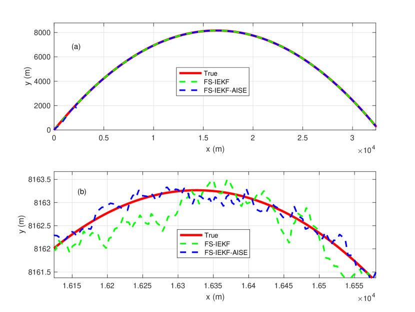
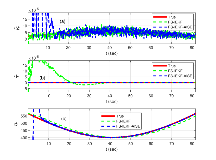
Table I shows the RMSE (45) for position, velocity, and the Frenet-Serret frame parameters for FS-IEKF and FS-IEKF-AISE. As shown, the RMSE for FS-IEKF-AISE is consistently lower across all metrics (position, velocity, and Frenet Serret frame parameters) when compared to FS-IEKF. Figure 3 shows the estimated position, with (b) providing a zoomed view of (a), showing that FS-IEKF-AISE closely tracks the true position compared to FS-IEKF. Figure 4 shows the estimated Frenet-Serret parameters.
| FS-IEKF | FS-IEKF-AISE | |
| 10.95 | 2.75 | |
| 7.24 | 1.77 | |
| 9.17 | 1.96 | |
| 6.82 | 1.67 | |
| 5.5e5 | 2.5e5 | |
| 2.7e3 | 1e10 | |
| 11.30 | 1.95 |
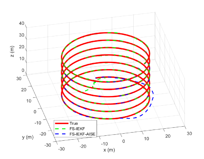
Example IV.2
Target Tracking for a Helical Trajectory. In this simulation scenario, the target follows a helical trajectory. The discretetime equations governing the trajectory are defined as
| (47) |
where s. To simulate the noisy measurement of the target position , white Gaussian noise is added to position measurement, with standard deviation m.
For FS-IEKF, , is set to a value that is within a small margin of the true value, , , and . For FS-IEKF-AISE with single differentiation, the parameters are the same as those used in Example IV.1 except that . For the cases of double and triple differentiation using AISE and IEKF, the parameters are the same as those used in Example IV.1.
Table II shows the RMSE values (45) for the position, velocity, and Frenet-Serret frame parameters for both FS-IEKF and FS-IEKF-AISE. FS-IEKF-AISE achieves performance comparable to FS-IEKF, as expected. This is because, for the helical trajectory, the Frenet-Serret parameters remain constant over time, making the constant parameter assumption in FS-IEKF valid for this case. Figure 5 shows the estimated position. Figure 6 shows the estimated Frenet-Serret parameters using FS-IEKF and FS-IEKF-AISE.
| FS-IEKF | FS-IEKF-AISE | |
| 0.111 | 0.105 | |
| 0.107 | 0.111 | |
| 0.121 | 0.078 | |
| 0.309 | 0.588 | |
| 0.292 | 0.536 | |
| 0.401 | 0.431 | |
| 0.0012 | 0.0049 | |
| 0.001 | 0.003 | |
| 0.232 | 0.274 |

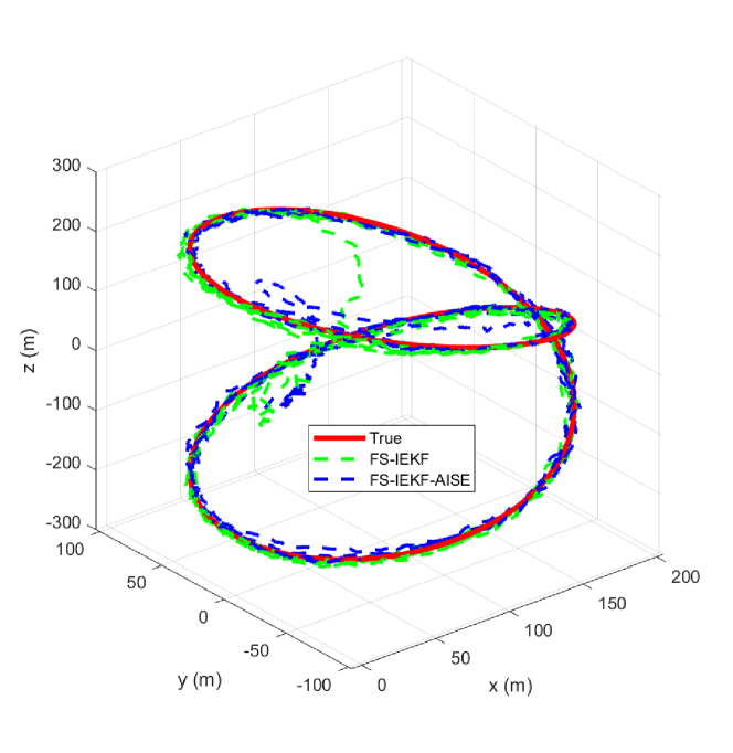
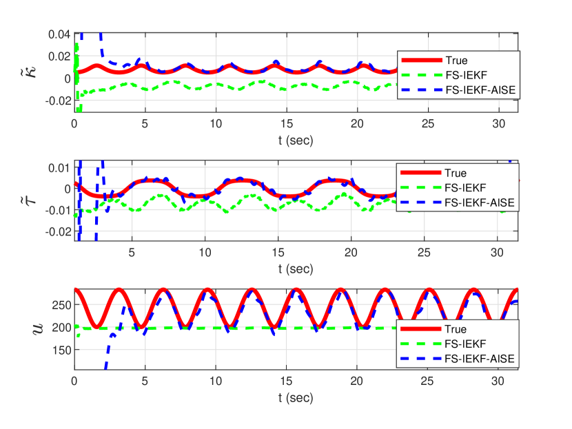
Example IV.3
Target Tracking for the Viviani Trajectory. In this simulation scenario, the target follows the Viviani trajectory. The discretetime equations governing the trajectory are defined as
| (48) |
where s. To simulate the noisy measurement of the target position , white Gaussian noise is added to position measurement, with standard deviation m.
For FS-IEKF, , and is set to a value that is within a small margin of the true value, , , and . In this example, the measurement noise is high, with a signal-to-noise ratio (SNR) of 20 dB. For FS-IEKF-AISE, for single differentiation using AISE, the parameters are the same as those used in Example IV.1 except that . All remaining parameters are same as in Example IV.1.
Table III shows the RMSE values (45). FS-IEKF-AISE consistently achieves the lower RMSE values for all metrics except for when compared to FS-IEKF. Figure 7 shows the estimated position. Figure 8 shows that, after the initial transient, the estimated Frenet-Serret parameters provided by FS-IEKF-AISE are more accurate than the estimates of FS-IEKF.
| FS-IEKF | FS-IEKF-AISE | |
| 9.53 | 3.72 | |
| 9.59 | 3.94 | |
| 12.54 | 4.15 | |
| 48.62 | 14.52 | |
| 45.57 | 14.15 | |
| 51.22 | 12.42 | |
| 0.015 | 0.0013 | |
| 0.008 | 0.015 | |
| 53.323 | 10.634 |
V Conclusions and Future Research
This paper proposed a novel target-tracking technique called FS-IEKF-AISE, which integrates the Frenet-Serret (FS) frame with adaptive input and state estimation (AISE) and the Invariant Extended Kalman Filter (IEKF). AISE is employed for real-time numerical differentiation on noisy position data to estimate velocity, acceleration, and jerk. These estimates are crucial for dynamically defining the torsion and curvature parameters of the FS frame, enabling the system to model complex, timevarying target trajectories without assuming constant motion parameters.
By applying IEKF to the FS frame, FS-IEKF-AISE achieves better accuracy compared to previous methods in estimating the target position and velocity. This approach not only enhances tracking performance in scenarios involving highly maneuverable targets but also preserves the group-affine structure of the system model, which has empirically improved convergence. Additionally, the FS-IEKF-AISE method ensures that the state evolution remains consistent within the Lie group framework.
Future work will focus on validating FS-IEKF-AISE in real-world applications. Finally, developing an adaptive IEKF that dynamically tunes the noise covariance will further enhance the accuracy of FS-IEKF-AISE in uncertain, timevarying operational conditions.
ACKNOWLEDGMENTS
This research supported by NSF grant CMMI 2031333.
References
- [1] M. Kumar and S. Mondal, “Recent developments on target tracking problems: A review,” Ocean Engineering, vol. 236, p. 109558, 2021.
- [2] P. Zarchan, Tactical and Strategic Missile Guidance (6th Edition). AIAA, 2012.
- [3] Y. Bar-Shalom, X. Li, and T. Kirubarajan, Estimation with Applications to Tracking and Navigation: Theory, Algorithms and Software. Wiley, 2001.
- [4] X. Rong Li and V. Jilkov, “Survey of maneuvering target tracking. part i. dynamic models,” IEEE Trans. Aero. Elec. Sys., vol. 39, no. 4, pp. 1333–1364, 2003.
- [5] M. U. Akcal and G. Chowdhary, “A predictive guidance scheme for pursuit-evasion engagements,” in AIAA Scitech Forum, 2021. AIAA 2021-1226.
- [6] M. Breivik, V. E. Hovstein, and T. I. Fossen, “Straight-line target tracking for unmanned surface vehicles,” Modeling, Identification and Control: A Norwegian Research Bulletin, vol. 29, no. 4, pp. 131–149, 2008.
- [7] Y. Chan, A. Hu, and J. Plant, “A kalman filter based tracking scheme with input estimation,” IEEE Trans. Aero. Elec. Sys., vol. AES-15, no. 2, pp. 237–244, 1979.
- [8] H.-M. Chuang, D. He, and A. Namiki, “Autonomous target tracking of UAV using high-speed visual feedback,” Applied Sciences, vol. 9, no. 21, p. 4552, 2019.
- [9] S. Ghosh and S. Mukhopadhyay, “Tracking reentry ballistic targets using acceleration and jerk models,” IEEE Trans. Aero. Elec. Sys., vol. 47, no. 1, pp. 666–683, 2011-01.
- [10] Y. Guo, Y. Yao, S. Wang, B. Yang, F. He, and P. Zhang, “Maneuver control strategies to maximize prediction errors in ballistic middle phase,” J. Guid. Contr. Dyn., vol. 36, no. 4, pp. 1225–1234, 2013-07.
- [11] R. Gupta, A. D’Amato, A. Ali, and D. Bernstein, “Retrospective-cost-based adaptive state estimation and input reconstruction for a maneuvering aircraft with unknown acceleration,” in AIAA 2012-4600, AIAA Guidance, Navigation, and Control Conf., 2012.
- [12] A. Ansari and D. S. Bernstein, “Input estimation for nonminimum-phase systems with application to acceleration estimation for a maneuvering vehicle,” IEEE Trans. Contr. Sys. Tech., vol. 27, no. 4, pp. 1596–1607, 2019.
- [13] L. Han, Z. Ren, and D. S. Bernstein, “Maneuvering Target Tracking Using Retrospective-Cost Input Estimation,” IEEE Trans. Aero. Elec. Sys., vol. 52, no. 5, pp. 2495–2503, 2016.
- [14] D. F. Hardiman, J. C. Kerce, and G. C. Brown, “Nonlinear estimation techniques for impact point prediction of ballistic targets,” in Proc. SPIE 6236, Signal and Data Processing of Small Targets, p. 62360C, 2006.
- [15] W. Harlin and D. Cicci, “Ballistic missile trajectory prediction using a state transition matrix,” Applied Mathematics and Computation, vol. 188, no. 2, pp. 1832–1847, 2007-05.
- [16] Hungu Lee and Min-Jea Tahk, “Generalized input-estimation technique for tracking maneuvering targets,” IEEE Trans. Aero. Elec. Sys., vol. 35, no. 4, pp. 1388–1402, 1999.
- [17] Y. Bar-Shalom, K. Chang, and H. Blom, “Tracking a Maneuvering Target Using Input Estimation Versus the Interacting Multiple Model Algorithm,” IEEE Trans. Aero. Elec. Sys., vol. 25, no. 2, pp. 296–300, 1989.
- [18] H. Khaloozadeh and A. Karsaz, “Modified input estimation technique for tracking manoeuvring targets,” IET Radar, Sonar & Navigation, vol. 3, no. 1, p. 30, 2009.
- [19] B. Lee, J. Park, Y. Joo, and S. Jin, “Intelligent kalman filter for tracking a manoeuvring target,” IEE Proc. Radar, Sonar and Navigation, vol. 151, no. 6, p. 344, 2004.
- [20] Y. Li, X. Li, and H. Wang, “Target Tracking in a Collaborative Sensor Network,” IEEE Trans. Aero. Elec. Sys., vol. 50, no. 4, pp. 2694–2714, 2014.
- [21] D. Tenne and T. Singh, “Characterizing Performance of -- Filters,” IEEE Trans. Aero. Elec. Sys., vol. 38, no. 3, pp. 1072–1087, 2002.
- [22] P. R. Kalata, “The Tracking Index: A Generalized Parameter for - and -- Target Trackers,” IEEE Conf. Dec. Contr., pp. 559–561, 1983.
- [23] J. E. Gray and W. J. Murray, “A Derivation of an Analytic Expres- sion for the Tracking Index for the Alpha-Beta-Gamma Filter,” IEEE Trans. Aero. Elec. Sys., vol. 29, no. 3, pp. 1064–1065, 1993.
- [24] P. Mookerjee and F. Reifler, “Reduced State Estimators for Consistent Tracking of Maneuvering Targets,” IEEE Trans. Aero. Elec. Sys., vol. 41, no. 2, pp. 608–619, 2005.
- [25] A. H. Hasan and A. Grachev, “Adaptive --filter for Target Tracking Using Real Time Genetic Algorithm,” J. Electrical and Control Engineering, vol. 3, pp. 32–38, 08 2013.
- [26] M. Pilté, S. Bonnabel, and F. Barbaresco, “Tracking the frenet-serret frame associated to a highly maneuvering target in 3d,” in 2017 IEEE 56th Annual Conf. Decision and Control (CDC), pp. 1969–1974, 2017.
- [27] A. Barrau and S. Bonnabel, “The invariant extended kalman filter as a stable observer,” IEEE Trans. Autom. Contr., vol. 62, no. 4, pp. 1797–1812, 2017.
- [28] P. Marion, J. Sami, B. Silvère, B. Frédéric, F. Marc, and H. Nicolas, “Invariant extended kalman filter applied to tracking for air traffic control,” in 2019 Int. Radar Conf. (RADAR), pp. 1–6, 2019.
- [29] J. Gibbs, D. Anderson, M. MacDonald, and J. Russell, “An extension to the frenet-serret and bishop invariant extended kalman filters for tracking accelerating targets,” in 2022 Sensor Signal Processing for Defence Conf. (SSPD), pp. 1–5, 2022.
- [30] P. Marion, J. Sami, B. Silvère, B. Frédéric, F. Marc, and H. Nicolas, “Invariant extended kalman filter applied to tracking for air traffic control,” in 2019 Int. Radar Conf. (RADAR), pp. 1–6, 2019.
- [31] A. J. Hanson and H. Ma, “Visualizing flow with quaternion frames,” in Proc. Conf. Visualization ’94, p. 108–115, IEEE, 1994.
- [32] S. Verma, B. Lai, and D. S. Bernstein, “Adaptive Real-Time Numerical Differentiation with Variable-Rate Forgetting and Exponential Resetting,” in Proc. Amer. Contr. Conf., pp. 3103–3108, 2024.
- [33] S. Verma, S. Sanjeevini, E. D. Sumer, and D. S. Bernstein, “Real-time Numerical Differentiation of Sampled Data Using Adaptive Input and State Estimation,” Int. J. Control, pp. 1–13, 2024.
- [34] R. Hartley, M. Ghaffari, R. M. Eustice, and J. W. Grizzle, “Contact-aided invariant extended kalman filtering for robot state estimation,” The Int. J. Robotics Research, vol. 39, no. 4, pp. 402–430, 2020.